Earthquake Hazard Safety Assessment of Existing Buildings Using Optimized Multi-Layer Perceptron Neural Network

Abstract

The latest earthquakes have proven that several existing buildings, particularly in developing countries, are not secured from damages of earthquake. A variety of statistical and machine-learning approaches have been proposed to identify vulnerable buildings for the prioritization of retrofitting. The present work aims to investigate earthquake susceptibility through the combination of six building performance variables that can be used to obtain an optimal prediction of the damage state of reinforced concrete buildings using artificial neural network (ANN). In this regard, a multi-layer perceptron network is trained and optimized using a database of 484 damaged buildings from the Düzce earthquake in Turkey. The results demonstrate the feasibility and effectiveness of the selected ANN approach to classify concrete structural damage that can be used as a preliminary assessment technique to identify vulnerable buildings in disaster risk-management programs.

1. Introduction

In civil engineering, reinforced concrete (RC) is considered to be one of the most frequently used building components that has a significant character in building structure. Calculating the earthquake threat of such constructions on a municipal scale, as a serious factor in any risk evaluation, is a costly, time consuming, and difficult job, particularly it is not thoroughly done in partially developed countries. The majority of existing buildings in seismic regions do not satisfy modern design code requirements and need to be upgraded accordingly to an appropriate level. For instance, in Istanbul, Turkey, as a high seismic area, around 90% of buildings are substandard, which can be generalized for other earthquake-prone regions in Turkey [1]. There are many methods available for seismic assessment of structures, which involve detailed structural analysis and design [2,3]. These detailed assessment methods consume more time when the assessment must be performed for many buildings [4]. To filter and prioritize the buildings for comprehensive, time- and resource-saving assessment, alternative Rapid Visual Screening (RVS) methods have been developed [5].

The first RVS methodology was proposed by the Federal Emergency Management Agency (FEMA), U.S.A, in 1988 as “Rapid Visual Screening of Buildings for Potential Seismic Hazards: A Handbook” [6]. Furthermore, in 2002, because of earthquake disasters in the 1990s, the methodology was modified to integrate the latest technological advancements [7].

RVS is a qualitative procedure that estimates structural scores for structures, which has been widely used in countries that suffer seismic events as a practical, decision-making, and simple tool for ranking buildings regarding seismic vulnerability considerations. However, existing RVS methods are mostly region- or country-based approaches that depend on specific region seismic features and suffer from inaccuracy. Therefore, it has attracted the interest of many researchers to develop and improve innovative and accurate methods. As a result of this effort, there are some studies on different RVS methods [8,9] and many proposed new RVS by using linear regression [10,11,12], Multi-criteria decision-making [13], Fuzzy logic [14,15,16,17]. There are other methods for the probabilistic seismic vulnerability of buildings in urban areas [18], modification of the empirical method for seismic vulnerability according to an analysis of the actual seismic performance of buildings in the city of Lorca, Spain [19], damage and change detection techniques of buildings using very high-resolution optical satellite images [20], and seismic vulnerability assessment of school buildings built by industrialized building systems [21], which shows the variety of works in seismic vulnerability assessment of buildings.

However, each of them is based on the expert’s opinion, uncertainties, or assumptions based on the linear relationship between parameters. The ANNs have the main capability to insert and organize outcomes of difficulties that have recognized input data to extract expectations regarding the solution of the similar kind of difficulties with unfamiliar input data immediately (e.g., [22]). The function for relating the input and the output is decided by the neural network and the amount of training it receives; as far as neural networks have a kind of universality [23], therefore, any function and relationship can be computed by a neural network.

In the current investigation, an initial framework to improve quickly the probable seismic performance and damage classification of existing RC buildings has been proposed.

2. Building’s Damage Inducing Parameters

In the proposed method by Yakut et al. [24] for vulnerability assessment of buildings, they assumed that all buildings involved in the inventory are exposed to a particular earthquake; therefore, the damage is only assessed on the basis of structural parameters. In other words, the damage is evaluated merely based on the structural responses and not taking into account the excitation factors. Regarding the characteristics of the damaged structures and the enormous number of the existing building stock, they proposed the following parameters, which are selected as the basic estimation parameters for this study too. A detailed description and a full discussion of the effect of these factors on the observed damage are given elsewhere [24,25,26].

2.1. Number of Stories (NS)

This is the total number of individual floor systems above the ground level. A study by Sucuoğlu et al. [1] noticed a clear indication that the number of stories is a very significant or perhaps the most dominant parameter in determining the seismic vulnerability of typical multistory concrete buildings in Turkey. Moreover, this parameter has a direct effect to natural time period of a building (T) [27] and can be computed for a concrete frame building or a shear wall building by using the expressions given below [28], where H is the height of the building and related to the number of stories:

$$T=0.075{\left(H\right)}^{3/4}concreteframebuilding$$

(1)

$$T=0.05{\left(H\right)}^{3/4}shearwallbuilding$$

(2)

2.2. Normalized Redundancy Score (NRS)

The redundancy indicates the degree of continuity of several frame lines to distribute the lateral forces throughout the structure system. The Normalized Redundancy Ratio (NRR) of a frame structure is calculated using Equation (3), where $A_{tr}$ is the tributary area for a typical column, $n{f}_x$ and $n{f}_y$ are number of continuous frame lines in the critical story in x and y directions and $A_{gf}$ is the area of the ground story. From the value of NRR, the following values on

Table 1. NRS Value Based on NRR.

NRS	NRR
1	$0\le NRR\le 0.5$
2	$0.5\le NRR\le 1.0$
3	$1.0<NRR$

are assigned to the NRS

$$NRR=\frac{A_{tr}(n{f}_x-1)(n{f}_y-1)}{A_{gf}}.$$

(3)

2.3. Soft Story Index (SSI)

Damage and collapse due to the soft story are most often observed in buildings while the lower level containing the concrete columns behaved as a soft story in that the columns were unable to provide adequate shear resistance during the earthquake [29]. The ground story usually has fewer partitions than the upper story, which is also one of the main reasons for soft stories. Soft story index is defined as the ratio of the height of first story (i.e., the ground story), $H_1$, to the height of the second story, $H_2$

$$SSI=\frac{H_1}{H_2}.$$

(4)

2.4. Overhang Ration (OR)

The existence of overhangs and balconies shifts the mass center of the building upward and thus, increase seismic forces and overturning moments. Based on different studies [30,31], it was observed that buildings with overhangs were damaged more severe damages compared to regular buildings. This fact can attract researchers to choose a case study in Turkey, where 70 to 80% of buildings have overhangs [30]. Since overhangs make load calculation of a building more complicated and decrease earthquake strength of the structure, therefore it is recommended to prevent constructing overhangs; otherwise, this will increase the earthquake effects [32].

The area beyond the outermost frame lines on all sides of a floor plan is defined as the overhang area. The summation of the overhang area of each story, $A_{ova}$, divided by the area of the ground story, $A_{gf}$, is defined as the overhang ratio

$$OR=\frac{A_{ova}}{A_{gf}}.$$

(5)

2.5. Minimum Normalized Lateral Strength Index (MNLSI)

The (MNLSI) is the basic shear capacity of the critical story. The contributions of the columns, structural walls and unreinforced masonry walls are considered on this index. This index is the minimum value of $A_{nx}$ and $A_{ny}$ from Equation (6), which are total normalized lateral in the x and y directions, respectively. Also, $A_{tf}$ corresponds to total story area above ground level

$$\begin{array}{c}\hfill A_{nx}=\frac{\mathsf{\Sigma }{\left(A_{col}\right)}_x+\mathsf{\Sigma }{\left(A_{sw}\right)}_x+0.1\mathsf{\Sigma }{\left(A_{mw}\right)}_x}{A_{tf}}\times 1000,\\ \hfill A_{ny}=\frac{\mathsf{\Sigma }{\left(A_{col}\right)}_y+\mathsf{\Sigma }{\left(A_{sw}\right)}_y+0.1\mathsf{\Sigma }{\left(A_{mw}\right)}_y}{A_{tf}}\times 1000.\end{array}$$

(6)

2.6. Minimum Normalized Lateral Stiffness Index (MNLSTFI)

The lateral rigidity of the ground story, which is usually the most critical story, represents the lateral stiffness of the story and is taken into account through (MNLSTFI), which is equal to the minimum of the indexes $I_{nx}$ and $I_{ny}$ computed for the in the x and y directions by using Equation (7), where ${\left(I_{col}\right)}_x$ and ${\left(I_{col}\right)}_y$ represent the moment of inertias of the columns, ${\left(I_{sw}\right)}_x$ and ${\left(I_{sw}\right)}_y$ show the moment of inertias of the structural walls about the x and y axes, respectively.

$$\begin{array}{c}\hfill I_{nx}=\frac{\mathsf{\Sigma }{\left(I_{col}\right)}_x+\mathsf{\Sigma }{\left(I_{sw}\right)}_x}{\mathsf{\Sigma }{A}_{tf}}\times 1000,\\ \hfill I_{ny}=\frac{\mathsf{\Sigma }{\left(I_{col}\right)}_y+\mathsf{\Sigma }{\left(I_{sw}\right)}_y}{\mathsf{\Sigma }{A}_{tf}}\times 1000.\end{array}$$

(7)

3. Artificial Neural Network (ANN)

ANNs are a kind of artificial intelligence application regarding the machine learning which has been applied by engineers for solving the challenges by using the general rules of human brain functions (e.g., memory, training). Consequently, using the ANNs make it likely to approximate the solution of difficulties like pattern recognition, organization, and estimation of functions by using the computers which use algorithms based on a dissimilar philosophy from traditional ones to overcome complicated difficulties affected by lots of factors [22].

Though, using the ANNs for solving the civil engineering challenges began in 1989 by Adeli and Yen [33], who used them in the structural design process. Though, the early use of ANNs for damage estimation was encouraged to structures by strong ground signals offered by Molas and Yamazaki [34] in the mid-1990s. They studied ANNs’ capability to estimate the seismic damage of wooden constructions quickly. Furthermore, they investigated the magnitude regarding the effect of seismic factors on the seismic damage by means of sensitivity examination. Caglar and Garip [35] trained a multi-layer perceptron (MLP) with a back-propagation (BP) algorithm by means of a database that was improved over a statistical process named P25 method. Their model was likewise examined over a verification set which establishes actual present RC constructions exposed to the 2003 Bingöl earthquake. The outcomes specified that the ANNs might forecast successfully the probable seismic performance level of current RC constructions, even if these constructions are not comprised in the dataset that was used regarding the preparation. Arslan [36] investigated the effect of structural parameters (like the amount of stories, the strength of concrete and steel, shear wall ratio, infill wall ratio) on the performance level of regular frame RC constructions under seismic excitation by means of ANNs. The data set regarding the preparation of the ANNs was created over the use of nonlinear pushover analyses. Later, Arslan et al. [37] applied data of 66 real four- to ten-story RC constructions, 19 structural input parameters, and numerous preparation algorithms, according to perceptron networks for estimating the earthquake performance level of present constructions. But it should be noted that the selected ANN models in his investigation are valid merely for the exact ranges of the database. Consequently, the estimation capacity and duration of each algorithm is expected to be less than that considered in their investigation when the selected constructions are enlarged.

A study by Morfidis et al. [38] investigated the optimum combination of 14 seismic parameters for damage state prediction using ANNs. A set of 30 RC buildings complying with provisions of Eurocode 8 for elevation and plan dimensions were modeled elastically, analyzed, and designed using linear behavior. Furthermore, with lumped plasticity models, the nonlinear behavior were modeled by 65 horizontal bidirectional ground motions. For training the ANNs, Multi-Layer Feedforward Perceptron networks were used. The Maximum Interstory Drift Ratio (MIDR) obtained from the 3D nonlinear time history analysis of 30 buildings subjected to 65 actual ground motions were selected as the damage index to provide the data for the training dataset. Their investigations for the methods adopted the Stepwise Method (Forward and Backward stepwise method) and the Weights method. They determined that a minimum of 5 seismic parameters should be used as inputs and substantiates the use of ANNs for damage prediction, but 11 to 14 parameters showed the best effective combinations.

Furthermore, research presented by Tesfamariam and Liu [39] highlights the use of eight different statistical techniques for damage classification using seismic induced damage data along with six building performance modifiers. For a risk-based seismic assessment, the integration of site seismicity, importance/exposure factor, and vulnerability are required. The seismicity factor (along with site specific soil conditions) can be obtained easily from seismic hazard maps and similarly for importance factor (derived from the occupancy of the building). The third factor, vulnerability, creates the challenge for engineers.

The procedure, described in the next section, is dedicated to a group of low- and mid-rise RC buildings to rank and evaluate their vulnerability. It can also be used for a single building to obtain an indication of its expected vulnerability during a significant earthquake. Such procedures are very appealing because training engineers need simple ways to quickly assess the vulnerability of a given building stock for which prioritization is needed in an accurate, expeditious, and adaptable way.

4. Methodology

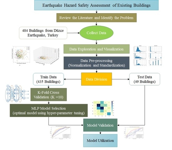
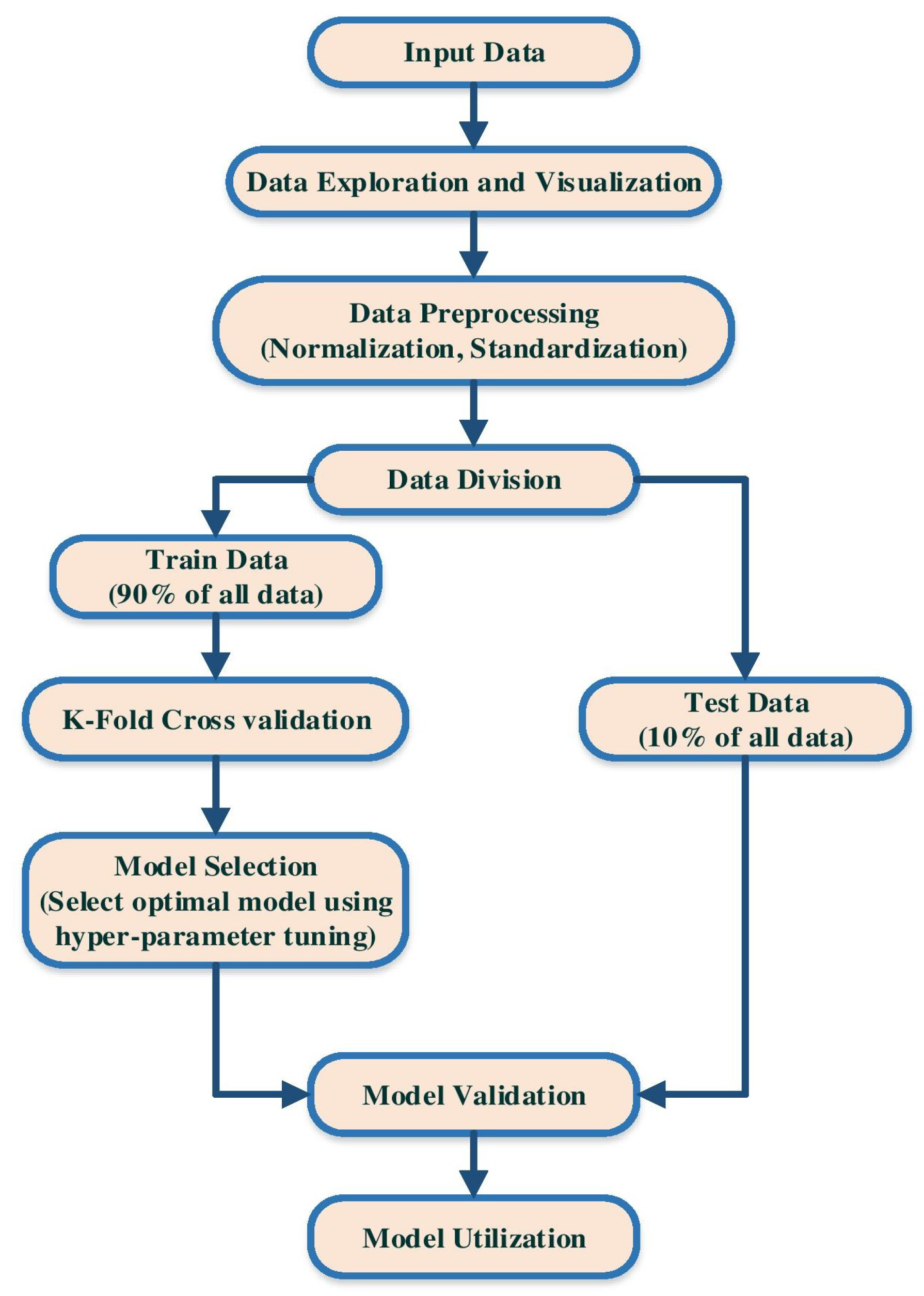
Figure 1 shows the workflow of this study on the classification of data of RC buildings. This workflow includes data preparation and visualization, model selection and model validation. Following are the deep explanation of all these steps in details. The process is suggested for low- to mid-rise reinforced concrete frame constructions with and without shear walls.

4.1. Data Preparation

The initial step in any machine-learning algorithm is data collection, cleaning and preparation for use in analysis. Data preparation consists of 4 parts:

4.1.1. Data Exploration and Visualization

Data exploration is the first stage in any data analysis, prediction, and organization tasks that naturally includes summarizing the main features of a data set, counting its size, data, initial patterns, and other characteristics to comprehend what is in a dataset and the features of the data. Moreover, by displaying data graphically, one can see if two or more variables correlated or not and determine if they are good candidates for other analyses includes univariate, bivariate, or multivariate analysis. This step also deals with missing values, data cleaning.

4.1.2. Data Pre-processing

This step deals with converting categorical data to numerical data and feature scaling. One-hot encoding is used to convert categorical variables to numerical to feed them to a model. On the other hand, feature scaling includes normalization and standardization; lack of data standardization leads to poor data, which has many negative effects on ANN [40]. Since the range of values of raw data varies widely, in ANN algorithms, objective functions will not work correctly without feature scaling. Another reason feature scaling is applied is that gradient descent converges much faster with feature scaling than without it [41]. The standardization method has been widely used for feature scaling in ANN [42]. Therefore, in this paper, standardization is applied to whole data using the following algorithm:

Standardization (or Z-score normalization) is the procedure of rescaling the characteristics so that they have the belongings of a Gaussian distribution with $\mu$ = 0 and $\sigma$ = 1, where $\mu$ is the mean and $\sigma$ is the standard deviation from the mean; standard scores (likewise named Z-scoring) of the examples are considered to be follows:

$$Z=\frac{x-\mu }{\sigma }.$$

(8)

When $Z=00$, the observation is at the sample’s mean (effect of centering) and when $Z=11$ then the observation is one standard deviation away from the mean (effect of normalizing) [43]. The advantages of Z-scoring are its simplicity and the possibility of ruling out outliers (winsorising) when the Z-score is extreme. It also keeps unchanged the sample correlation between features.

4.1.3. Data Division

The final objective regarding any machine-learning model is to study from examples in such a way that the model is accomplished of generalizing the learning to new examples, which it has not understood yet. Consequently, a dataset splits into two subsets as exercise and validation data. Once the model is primarily fit on a training dataset, the overview of a validation dataset throughout train procedure permits us to assess the model on different data than it is drill on and select the best model architecture. Lastly, the test data is still holding out for the last evaluation at the end of the model improvement for evaluating the model’s ability to generalize the unseen data. However, there is an alternative to this method, as called cross-validation, which only split data to train and test.

4.2. K-Fold Cross Validation

Cross-validation (CV) is used to generalize statistical analysis results from a set of model validation techniques to an independent data set. It tests the ability of the model to predict new data, assesses potential problems with the model, such as the overfitting of data or selection bias [44], and allows for the observation of the generalization technique of the model for unknown datasets. Generally, CV combines (averages) measures of fitness in prediction to obtain a more accurate estimate of model prediction performance [45]. K-fold cross-validation is the process with a single parameter named k that relates to the number of clusters that a given data sample (train data) is to be split into. Once a precise value for k is selected, it might be used in place of k in reference to the model, like k = 10 becoming 10-fold CV.

4.3. Model Selection

In this paper, a grid search algorithm applied to find the optimal hyper-parameters of the model. 10-fold cross-validation applied during the grid search process to avoid overfitting.

4.4. MLP Classifier Architecture

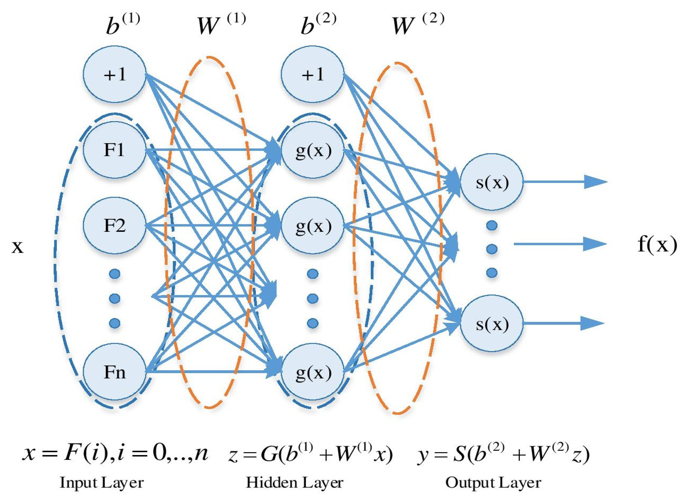
Figure 2 presents a structure of a typical MLP neural network with an input layer, one hidden layer and an output layer. Formally, a one-hidden-layer MLP is a function $f:R^M\to R^N$, where M is the size of input vector X and N is the size of the output vector $f\left(x\right)$, such that in matrix notation:

$$f\left(x\right)=G[b^{\left(2\right)}+W^{\left(2\right)}S(b^{\left(1\right)}+W^{\left(1\right)}x)],$$

(9)

with bias vectors $b^{\left(1\right)}$,$b^{\left(2\right)}$; weight matrices $W^{\left(1\right)}$, $W^{\left(2\right)}$ and activation functions $G,S$. The vector $h\left(x\right)=S(b^{\left(1\right)}+W^{\left(1\right)}x)$ constitutes the hidden layer. $W^{\left(1\right)}$ is the weight matrix connecting the input vector to the hidden layer. Each column $W^{\left(2\right)}$ represents the weights from the input units to the $ith$ hidden unit. Typical choices for G is $tanh$ or $Relu$ and for S include $tanh$, or the logistic sigmoid function.

4.5. MLP Hyper-Parameters

MLP has different hyper-parameters that cannot be learned during the training procedure. For example, the number of layers, number of neurons in each layer, learning rate, and activation functions are hyper-parameters that are predefined by the user before training. However, the selection of these parameters is crucial in terms of accuracy and generalization of the models. Therefore, automatic hyper-parameter tuning, e.g., greed search or random search, is recommended to optimize these hyper-parameters.

4.6. Hyper-Parameter Tuning Methods

Grid search, random search, and Bayesian search are some methods of optimization which are used to navigate the hyper-parameters space and tune MLP hyper-parameters. Each of these methods have their pros and cons. For example, grid search is fast. Still, it only applied to some finite points in hyper-parameters space, or Bayesian search set a prior over hyper-parameter distribution and sequentially update it while observing different experiments, which allows fitting hyper-parameters space better, but it is slower than grid search with small space. However, using any of these methods besides cross-validation leads to better results and accurate prediction of MLP.

Score Metrics

The most crucial parameter for classification problems is to decide which metric should be used to score the accuracy of the model. It could be an accuracy percentage, R-squared, adjusted R-squared, confusion matrix, F1, precision, recall, variance, regarding the type of classification problem as binary, multi-class, or multi-label classification. It is also essential to know that some of these metrics are sensitive to the structure of data. As an example, accuracy is not a useful metric for imbalanced data where the number of samples in each class are not equal. In this paper, average accuracy and receiver operating characteristic (ROC) curves are used to evaluate model performance as the earthquake damage is a multi-class problem with an imbalanced class where the damaged building divided into five categories as none, light, moderate, severe, and collapse. A ROC curve is a graph of true positive rate (sensitivity) versus false positive rate (specificity) for a binary classifier system. ROC curves typically feature a true positive rate on the Y-axis and false positive rate on the X-axis. The upper left corner is defined as a false positive value of 0 and a true positive value of 1, meaning that all positives found in this corner are true positives. Curves plotted on ROC graphs with a higher area under the curve (AUC) are considered to be more desirable results, indicating that the classifier used was a good fit for the dataset. This similarly specifies that the classifier is more probable to find true positives than true negatives. Then, the closer the curve follows the left-hand edge and then the top edge of the ROC space, the more precise the total classification. A perfect classification will have a zero false alarm amount and a 100% likelihood of discovery. ROC curves are generally used in binary arrangements to examine the output of a classifier. For extending the ROC curve and ROC area to multi-class, it is essential to binarize the results. One ROC curve could be drawn per class, but one might likewise draw a ROC curve by seeing each component of the class indicator matrix as a binary prediction.

4.7. Model Validation and Use

After model selection, the resulted optimum model applied to the test dataset, which is an unseen dataset during the training procedure. This test data examines the generalization of the model. The model used on the test dataset and the result considered to be a measure for future unseen data.

A multi-layer perceptron (MLP) is a class of feedforward ANN [46]. An MLP is a network of simple neurons called perceptrons, which computes a single output from multiple real-valued inputs by forming a linear combination according to its input weights and then possibly putting the output through some nonlinear activation function [46]:

$$y=\phi \left(\sum _{i=1}^n{w}_i{x}_i+b\right)$$

(10)

where the vector of weights is represented by w, x denotes the vector of inputs, b is the bias and $\phi$ is the activation function.

The most commonly used activation functions are logistic sigmoid and tanh. These functions are used because they are mathematically convenient and are close to the near-linear origin while saturating quite quickly when they move away from the origin. This allows MLP networks to model well both strongly and mildly nonlinear mappings.

Multi-layer perceptrons that are trained by means of datasets of input-output pairs, learning to model the correlation or dependencies among members of each pair, are usually used to supervise learning difficulties. Training contains regulating the parameters, or the weights and biases, of the model to decrease the error rate. Back-propagation is applied to make those weight and bias modifications relative to the error, and the error itself could be measured in several manners, counting by root mean squared error (RMSE). In the forward pass, the signal flow transfers from the input layer over the hidden layers to the output layer, and the choice of the output layer is measured against the ground truth labels.

5. Results and Discussion

The proposed methodology applied to different MLP architectures to find the optimal model. The classification of damage data is carried out using Scikit-learn [47] as it is the well-maintained, comprehensive, and open-sourced machine learning package in Python programming language.

5.1. Dataset

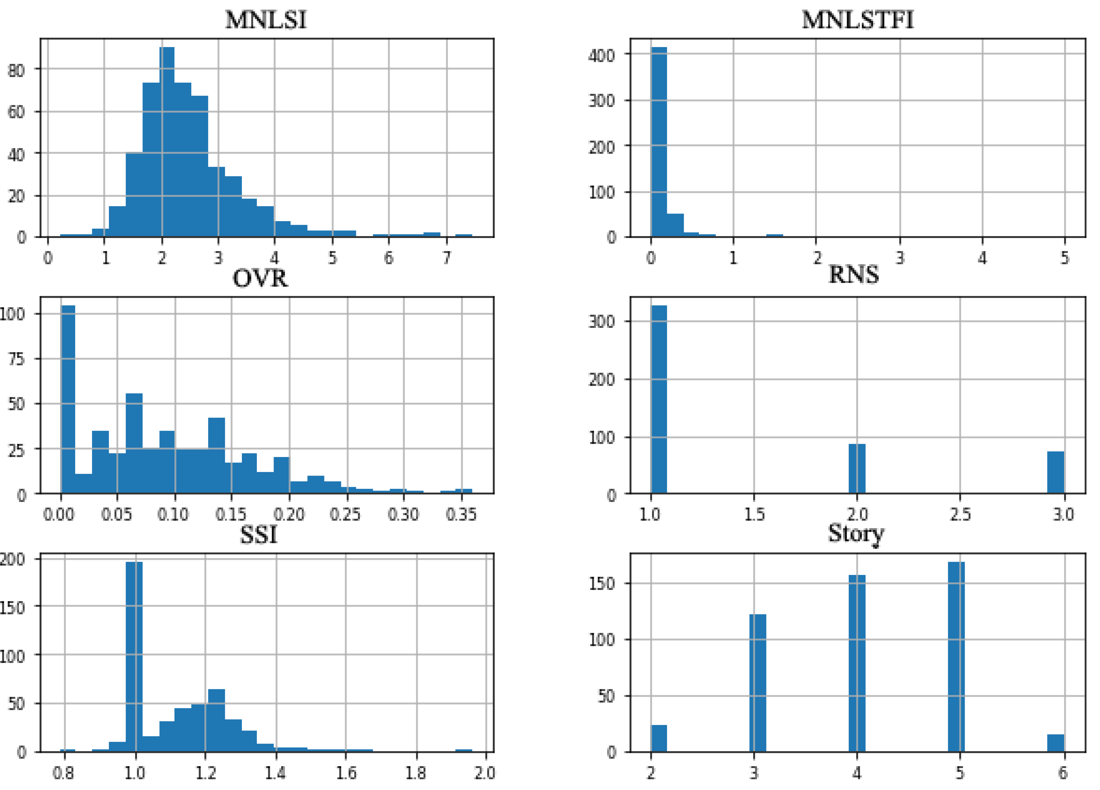
On 12 November 1999, a powerful earthquake $M_w$ = 7.1 struck the city of Düzce (Turkey) within a PGA approximately 0.821 g and PGV of 66.9 m/s [48]. The Düzce earthquake dataset of 484 data and 6 variables is used to train and validate the model. This dataset is from the SERU (Structural Engineering Research Unit) [49], and compiled from damage surveys conducted after the 1999 Düzce earthquake. Moreover, Düzce is located on the northwest of Turkey under a high seismic zone, and the soil conditions were stiff clays with interbedded layers of dense sands and gravels. Six input variables considered in this dataset, which are MNLSI, MNLSTFI, OVR, RNS, SSI, and Number of Stories, as described beforehand. Figure 3 shows the distribution of each data for each input where MNLSI, OVR, Story numbers and SSI follows a Gaussian distribution while others are not normally distributed. As can be seen, most of the buildings had 3 to 5 stories, and OVR is high for many buildings, and the same is for SSI. In contrast, MNLSTFI of buildings was mainly less than 1, although MNLSI was extremely distributed between 1 and 4.

The observed structural damage states of data were categorized into 5 categories based on the descriptions given in

Table 2. Description of Damage.

Damage State	Damage Grade	Structural Elements
None	1	No visual sign of damage
Light	2	Hairline inclined or flexural cracks
Moderate	3	Concrete spalling
Severe	4	Local structural failure
Collapse	5	Local or total collapse

.

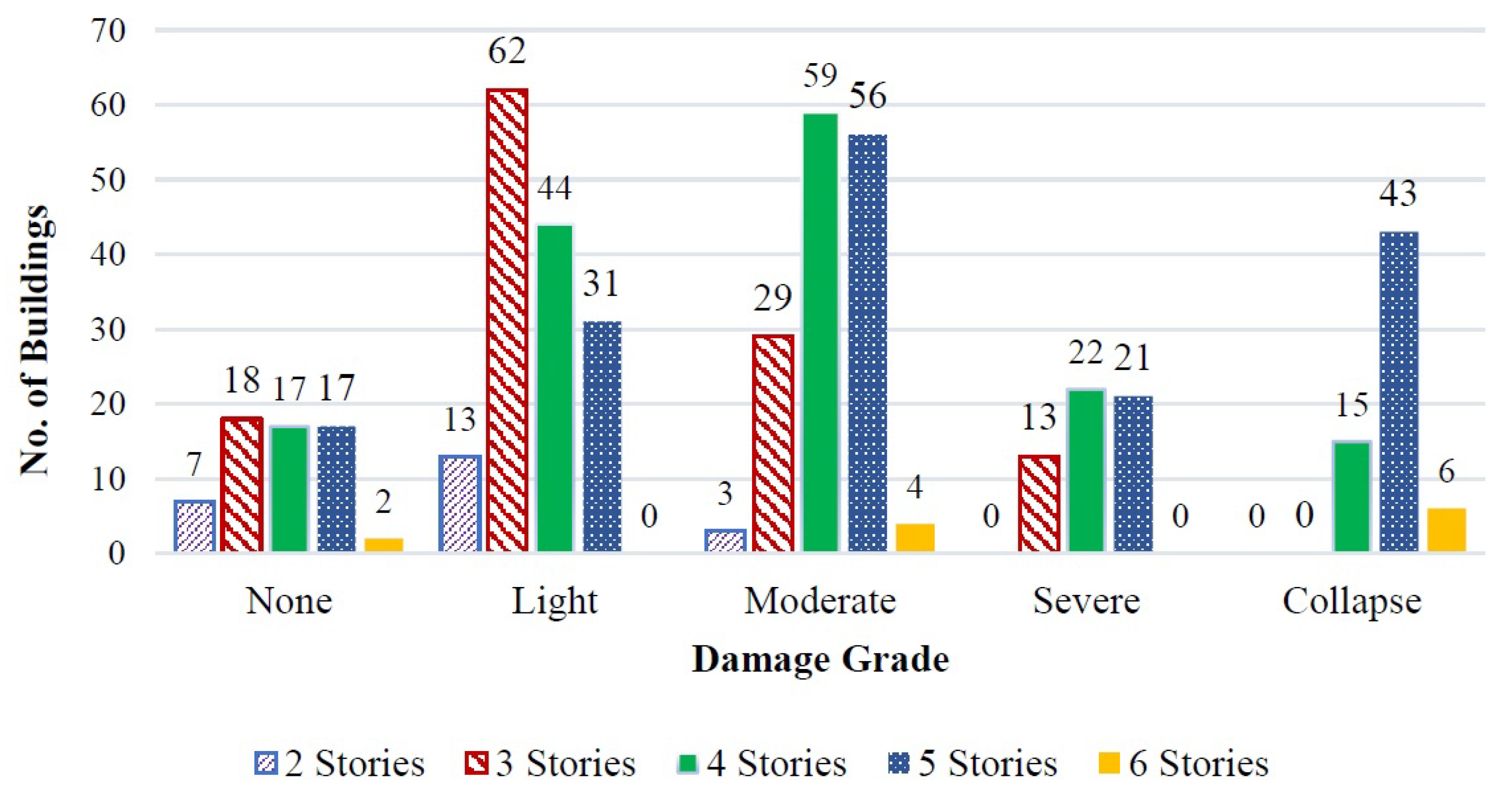
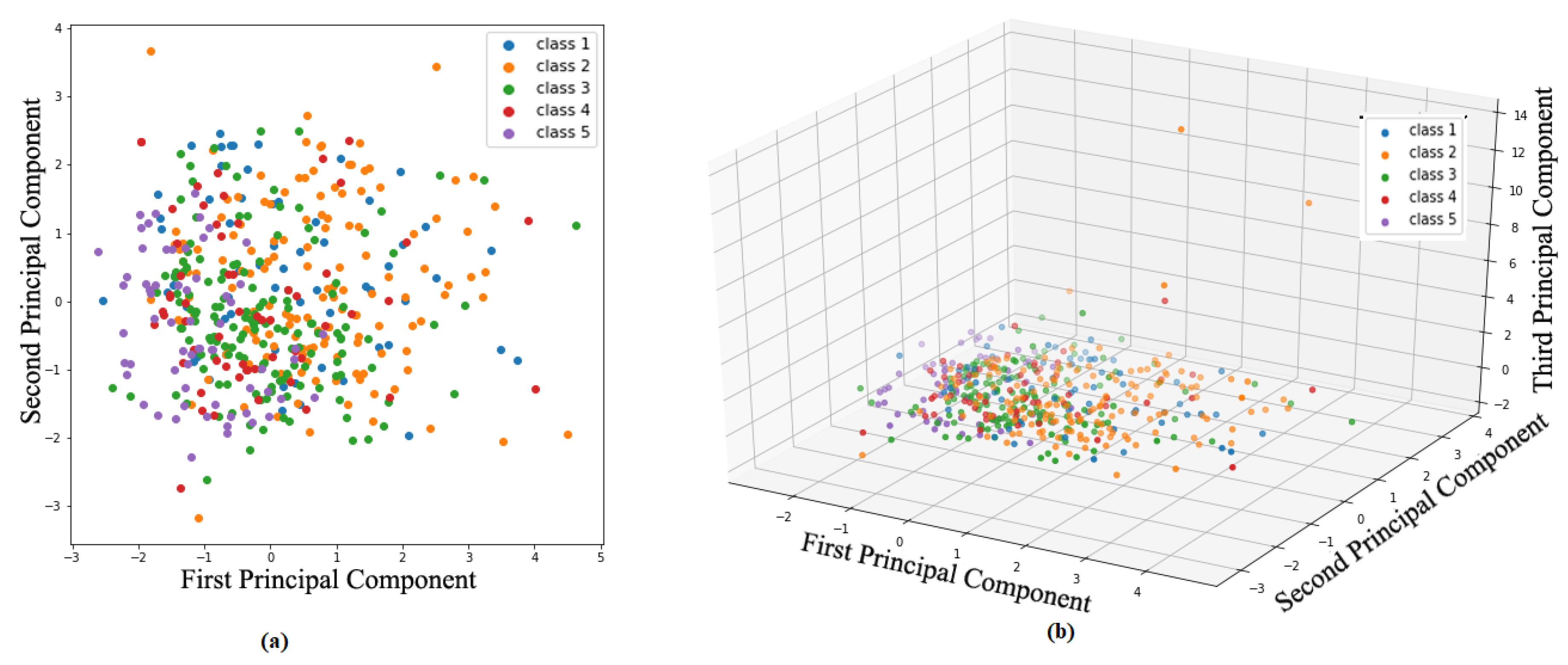
As an example, Figure 4 demonstrates the distribution of studied buildings according to the number of stories and the observed damage. As can be seen, the majority of damages are for 4 and 5 stories buildings, and most of the buildings have damaged within grades 2 and 3. It indicates that by raising the number of stories, the vulnerability increase too. Figure 4 illustrated a total of 61 instances are labeled with Class 1 (none), 145 instances with Class 2 (light), 147 instances with Class 3 (moderate), 60 instances with Class 4 (severe) and the remaining 63 instances are labeled with Class 5 (collapse). This is an example of an imbalanced multi-class problem where the number of building in Class 2 and Class 3 are more than other damaged classes. Therefore, using accuracy maybe leads to a wrong decision about the model performance and other metrics like average accuracy is a better option. Principal component analysis (PCA) was used to explore the difficulty of the data classification and visualize the data distribution. Figure 5a,b shows the data distribution in 2D and 3D. It can be seen visually that the classification of data is a difficult task as it is too nonlinear and have a mixed class.

Most of the data lay on a plate and do not have high variance in the third dimension; even in this 2D plate, some classes are mixed, which makes it difficult for any classification method to categorize these data.

5.2. Dataset Pre-Processing

Data pre-processing is an important step to prepare the data for further purposes and improving the quality of the raw experimental data [51]. There are many important steps in data pre-processing, such as data cleaning, data transformation, and feature selection [52]. Here, the data preparation step only includes standardization based on Equation (8) as this dataset does not include any categorical data.

5.3. Dataset Division

484 data divided into two parts as train and test. Here, 90% of data assigned to train dataset, and 10% hold as test dataset. Then, 10-fold cross-validation applied to train data. It means that first, the train data shuffled randomly and separated into 10 parts or folds. Then, the model trained on 9 folds, and one fold is held out for validation. This procedure repeated 10 times, and each time one fold is kept for validation.

5.4. Model Selection

A combination of different hyper-parameters has been considered to find the best model. In this study, a grid search is used to find an optimum model. 10-fold cross-validation applied on each node of the grid, and the score of each model is calculated based on the average error of the model on all folds. Finally, a model with the lowest average error is considered to be the best model and applied on a separate test dataset to find its generalization. The hyper-parameter values of MLP neural network, which considered in this study is shown in

Table 3. Hyper-parameter Values.

Hyper-Parameter	Values
Hidden Layer sizes	(15,10); (20,10); (15,10,5); (20,15,10)
Activation Function	Tanh; Relu
Solvers	Sgd; adam; lbfgs
$\alpha$	0.0001; 0.001; 0.01; 0.1
Maximum Iteration	500; 1000; 1500
Learning Rate	Constant; Adaptive

. After applying the grid search algorithm on Table 3 hyper-parameters, the final model has been selected with the lowest error on the train dataset.

Table 4. Hyper-parameter Results.

Hyper-Parameter	Values
Hidden Layer sizes	(25,15,10)
Activation Function	tanh
Solvers	adam
$\alpha$	0.01
Maximum Iteration	500
Learning Rate	Constant

shows the best hyper-parameters of final model.

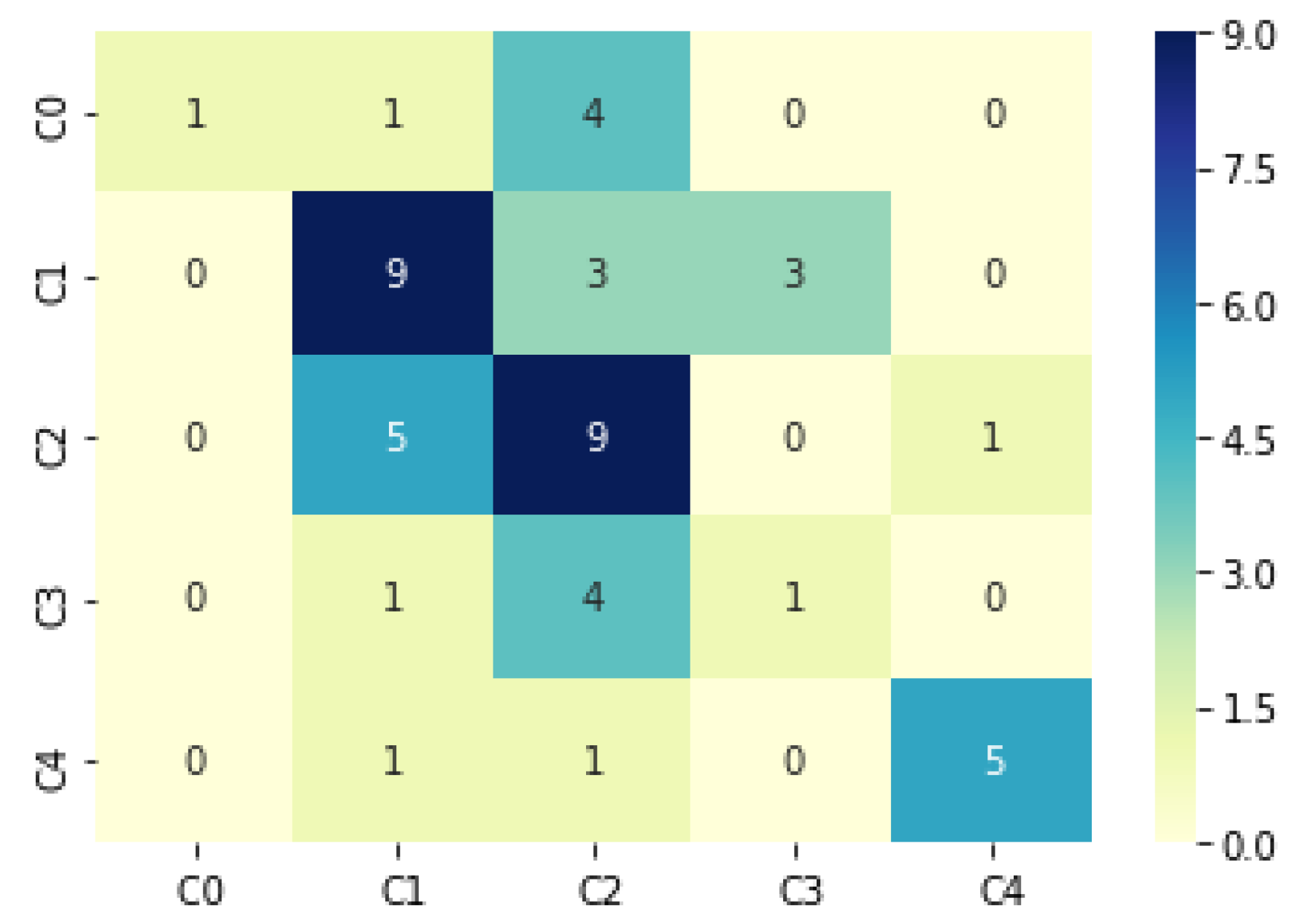
Figure 6 shows the confusion matrix by class support size (number of elements in each class). Numbers which appear on the diagonal of the matrix represent the number of cases where the MLP accurately classified (predicted) the classification in comparison to the actual classification. Those numbers which appear elsewhere in the matrix represent misclassifications by the MLP. Therefore, the higher the numbers in the diagonal, the more accurate the MLP algorithm predicted the building classification. The overall accuracy from the Figure 6 is around 0.52, which in the previous study by Tesfamariam [39] in this area of research has reported 0.45.

As can be seen from the confusion matrix, Class 5 has more correctly classified (5 out of 7) buildings compare to others, while Class 1 is where model has more incorrect classified buildings (4 out of 6). It means that the model has a great ability to recognize most vulnerable buildings while it has less accuracy in categorizing good condition buildings. The classification result for damage state is binary, e.g., (1,0,0,0,0) means Class 1 or no damage. 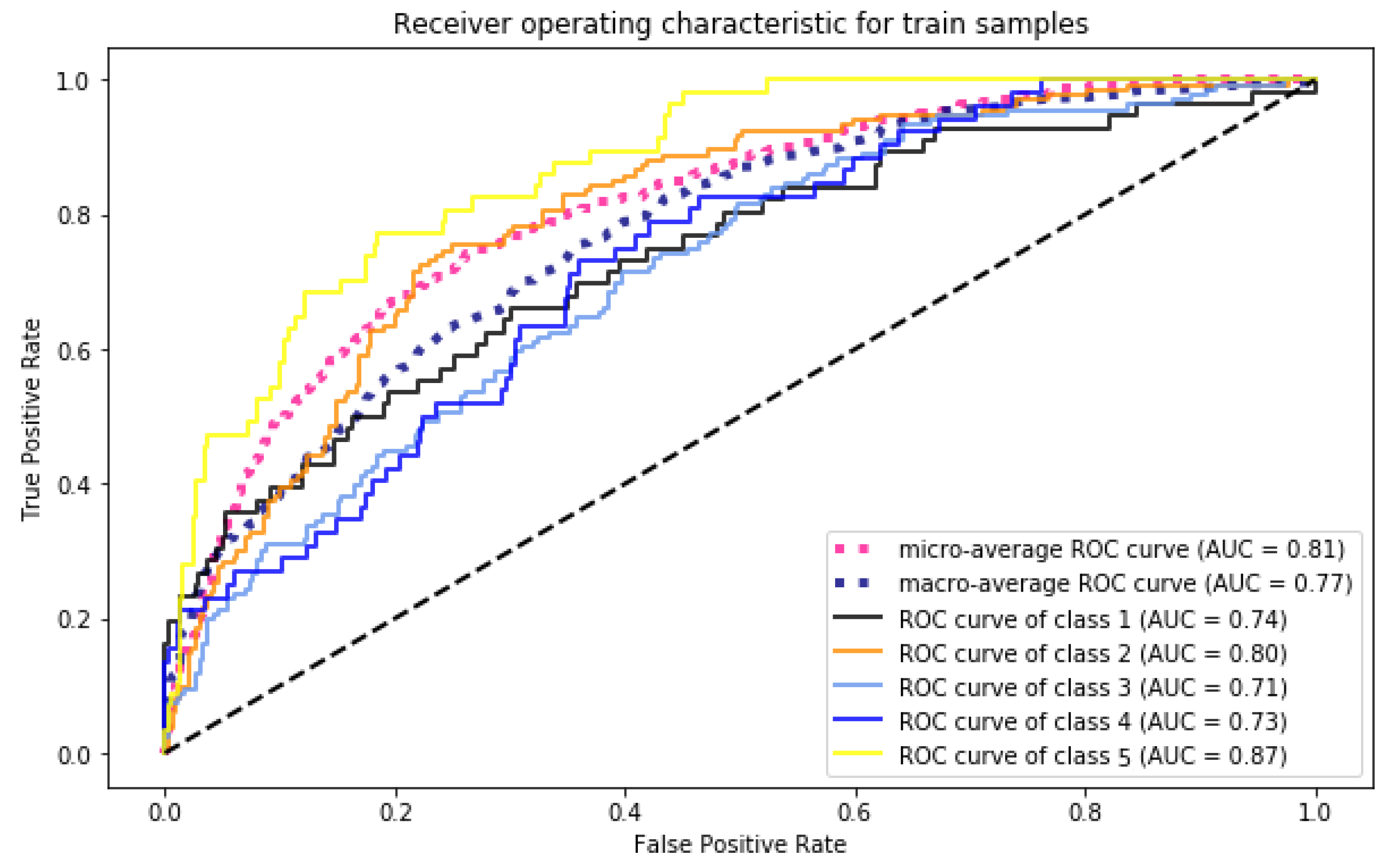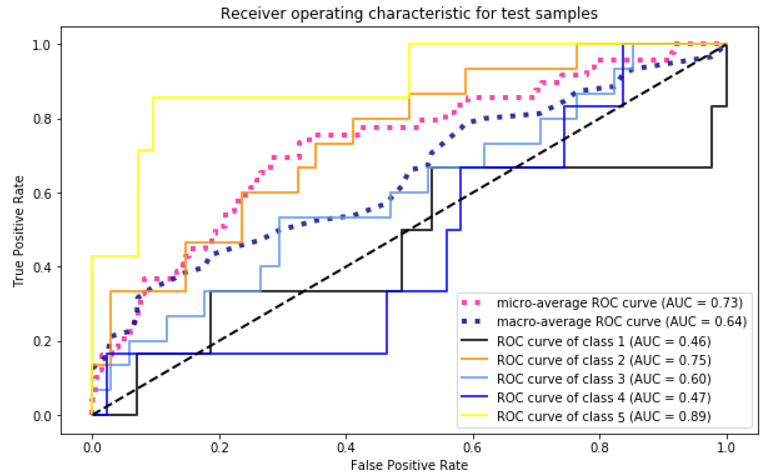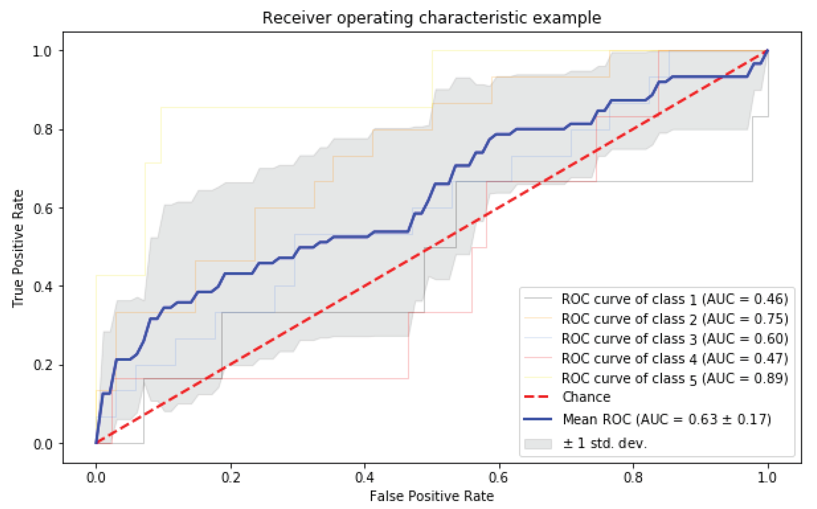Figure 7 and Figure 8 are presenting the ROC curves of the train and test samples for all classes, respectively, besides micro and macro average. Additionally, in Figure 9, the mean ROC has been presented.

As is clear from Figure 7, all classes have a high AUC, which means that the model well fitted on the train dataset. The AUCs of Class 1 to 5 are 0.74, 0.80, 0.71, 0.73 and 0.87, respectively. This means that the model has an accuracy higher than 0.71 for conditions that match the train dataset. On the other hand, Figure 8 shows the AUC results by applying the model to the test dataset. The AUCs of Class 1 to 5 are 0.46, 0.75, 0.6, 0.47, 0.89, respectively. Compared to train results, it determines that the generalization of the model is appropriate for classes 2, 3, and 5 while it is not well suited for Class 1 (NO Damage) and 4 (Severe Damage). The ROC curves of Figure 8 also shows that the model has worst results (less than random model) on Class 1 and 4 where the curve of these to class is below than the dashed line. Looking at the confusion matrix shows that most of the buildings in these classes (Class 1 and 4) incorrectly classified as Class 3 (Moderate). It means that the feature of Class 3 is very similar to Class 0 and 3. Therefore, for this dataset, MLP able to classify most vulnerable buildings; however, it is not possible to classify buildings with sever damages correctly, which is a drawback of the model.

6. Conclusions

Though most of the fast-growing city expenditures were typically situated in seismic-prone areas throughout recent decades, seismic threat-sensitive urban planning and seismic-resistant building was not the maximum priority during this evolution stage. Due to the large number of buildings, there is a need for retrofit prioritization, and a risk-based prioritization is desirable. In this paper, a classification technique based on neural networks and the application of six performance modifiers, N, SSI, OHR, MNLSTFI, MNLSI, and NRS, has been illustrated. In addition, it should be mentioned that the accuracy of the study depends on the sample buildings chosen, the calculation methods, and the parameters that are present during the ANN instruction and testing processes. The proposed method helps to manage and implement strategies for the safety of the communities before an earthquake event takes place by investigating the vulnerability classes for each building and identifying highly vulnerable buildings that deserve further inquiry. Results show that an optimized MLP model with three hidden layers (25, 15, 10) has a high accuracy in detecting most vulnerable buildings (grade 5) but a low accuracy on severely damaged buildings (grade 4). Therefore, adding more variables (parameters that have an influence on the structural behavior) to the input data leads to higher accuracy.