Article

Physical Scaling of Oil Production Rates and Ultimate Recovery from All Horizontal Wells in the Bakken Shale

The Ali I. Al-Naimi Petroleum Engineering Research Center, King Abdullah University of Science and Technology, Thuwal 23955-6900, Saudi Arabia
*
Author to whom correspondence should be addressed.
Energies 2020, 13(8), 2052; https://doi.org/10.3390/en13082052
Submission received: 17 February 2020 / Revised: 7 March 2020 / Accepted: 11 March 2020 / Published: 20 April 2020

Abstract

:
A recent study by the Wall Street Journal reveals that the hydrofractured horizontal wells in shales have been producing less than the industrial forecasts with the empirical hyperbolic decline curve analysis (DCA). As an alternative to DCA, we introduce a simple, fast and accurate method of estimating ultimate recovery in oil shales. We adopt a physics-based scaling approach to analyze oil rates and ultimate recovery from 14,888 active horizontal oil wells in the Bakken shale. To predict the Estimated Ultimate Recovery (EUR), we collapse production records from individual horizontal shale oil wells onto two segments of a master curve: (1) We find that cumulative oil production from 4845 wells is still growing linearly with the square root of time; and (2) 6401 wells are already in exponential decline after approximately seven years on production. In addition, 2363 wells have discontinuous production records, because of refracturing or changes in downhole flowing pressure, and are matched with a linear combination of scaling curves superposed in time. The remaining 1279 new wells with less than 12 months on production have too few production records to allow for robust matches. These wells are scaled with the slopes of other comparable wells in the square-root-of-time flow regime. In the end, we predict that total ultimate recovery from all existing horizontal wells in Bakken will be some 4.5 billion barrels of oil. We also find that wells completed in the Middle Bakken formation, in general, produce more oil than those completed in the Upper Three Forks formation. The newly completed longer wells with larger hydrofractures have higher initial production rates, but they decline faster and have EURs similar to the cheaper old wells. There is little correlation among EUR, lateral length, and the number and size of hydrofractures. Therefore, technology may not help much in boosting production of new wells completed in the poor immature areas along the edges of the Williston Basin. Operators and policymakers may use our findings to optimize the possible futures of the Bakken shale and other plays. More importantly, the petroleum industry may adopt our physics-based method as an alternative to the overly optimistic hyperbolic DCA that yields an ‘illusory picture’ of shale oil resources.

Graphical Abstract

1. Introduction

In early 2019, seven major shale plays in the US produced nearly 70% of total US oil production. The Bakken shale is the second largest oil-producing play that in mid-2019 produced 1.45 million bbl of oil per day from 14,888 active horizontal hydrofractured wells. Therefore, it is important to have a reliable predictive model of oil production and ultimate recovery in the Bakken and other shale plays. In shale or tight oil reservoirs, where drainage area and communication between wells are limited [1,2], the estimated ultimate recovery (EUR) per well is the key indicator used to assess fieldwide production potential. The most popular way of predicting EUR from a shale well is the traditional decline curve analysis (DCA) proposed by Arps [3] 75 years ago. This method is favored by the industry, because it only requires production data to forecast future performance of each well and it is easy to implement for many wells. Most published fieldwide predictions of EUR use DCA. Good examples are the Bakken predictions by the US Geological Survey [4,5] and US DOE Energy Information Administration [6].
In his seminal paper, Arps [3] stated that DCA works by extrapolating oil rate observed in a pseudo-steady state (boundary-dominated) flow regime. Unfortunately, because of the vanishing matrix permeability, shale wells do not reach pseudo-state flow regime during their entire existence. Thus, traditional DCA commonly overestimates EURs of shale wells [7,8]. In early 2019, an analysis published by the Wall Street Journal (WSJ) revealed that 2/3 of the projections made by shale companies appeared to be overly optimistic [9,10]. Thousands of shale wells drilled between 2014 and 2017 are pumping on average 10% less oil and gas than their owners’ forecasts. In certain regions, the discrepancy between forecasts and actual production is more than 50%. The total deficit is equivalent to one billion barrels of oil and gas that will not be produced over 30 years or to $30 billion at current oil price.
Several authors have suggested alternatives to the traditional DCA. These are, e.g., the Power Law Exponential Decline [11], the Stretched Exponential Decline [12,13], the Logistic Growth Model [14], the Bayesian probabilistic DCA [15,16], and the Extended Exponential DCA [17]. Empirical models are simple, but they also are mere curve fits, whose parameters have little physical meaning and cannot be generalized. In hyperbolic DCA, for example, the exponent b is adjusted to fit production data, notwithstanding several studies that have tried to elucidate its physical meaning [18,19,20]. Another limitation of most empirical models is their inability to capture the two regimes of oil and gas production in shales that are transient-linear flow at early times and boundary-dominated flow at later times on production [21]. We posit that the physics-based analytic or numeric solutions (such as [22,23]) are more predictive than the empirical decline curves. Unfortunately, many analytical solutions proposed in recent years are unpopular because of their complexity and large quantities of input data.
In this paper, we reintroduce our physics-based scaling approach that is based on an analytical solution of transient oil flow. In several other papers, notably in [14,21,24,25,26,27], we have reviewed the vast literature on this subject and, to avoid repetition, we omit it here. The physical scaling approach was originally developed to predict gas production in the Barnett shale [24,25]. In 2017, we extended our earlier gas production scaling to predict EURs from thousands of oil wells in the Eagle Ford [28]. In this paper, in turn, we extend the Eagle Ford scaling to predict EURs from the 14,888 existing horizontal, hydrofractured black oil wells in the Bakken. We consider the simplest model of oil production consistent with the first order physics and idealized geometry of the extraction process. In principle, the solution of this model depends on many parameters, but in practice—for a given shale play—all but two can be fixed at a field region-average values, resulting in an exact solution of a linearized transient pressure diffusion problem with simplified geometry of the hydrofractured horizontal wells as the boundary condition. At early times, the scaled oil production rate declines as one over the square root of dimensionless time on production, reflecting transient oil flow. Later, oil production rate declines exponentially indicating boundary-dominated flow. In addition, we combine the physical scaling approach with time superposition to resolve erratic production records of the refractured old Bakken wells, and of the wells that were put on artificial lift with time-varying downhole conditions.
To predict EURs, we collapse production records from individual horizontal oil wells onto two different segments of an almost universal scaling curve. The scaling is easy to program and works perfectly for large production data sets. Even though our approach is mechanistic, it preserves the simplicity of traditional DCA by relying only on average reservoir rock and fluid properties and on well-by-well time series of oil production. In a slightly different context, our physical scaling approach has been proven to have the same predictive power as full reservoir simulation, while being several orders of magnitude faster [29]. The EURs calculated from the physical scaling are compared with the latest results published by EIA.
We map water cuts, gas–oil ratios, and calculated EURs of Bakken wells to locate the best producing region in the Williston basin. We also analyze how recent advancements of well completion technologies influence EUR. Operators and policymakers may use our findings to guide sensible development of the Bakken and other shale plays. More importantly, petroleum industry may adopt our simple, fast and accurate method to predict oil production in shales as an alternative to the overly optimistic hyperbolic DCA that yields an ‘illusory picture’ of shale oil resources [9].

2. Materials and Methods

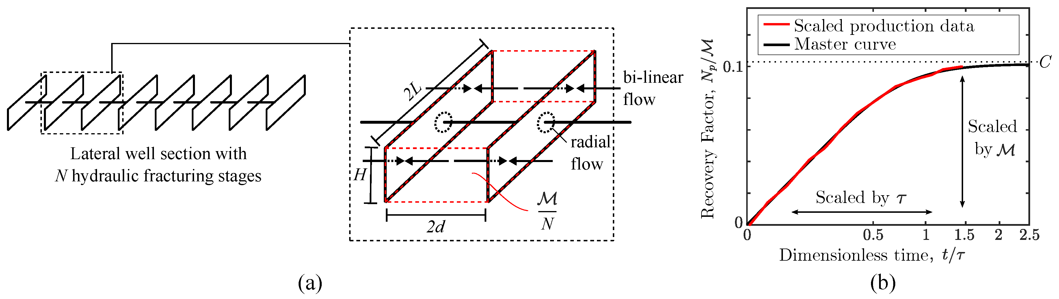
2.1. Physical Scaling

The physical scaling approach extended in this paper was first derived in the paper SPE-187226 [28], and used to predict oil production from thousands of horizontal wells in the Eagle Ford shale play. The scaling solution given in SPE-187226 is based on an assumption that oil is produced from a hydrofractured shale well under a natural depletion mechanism (Section 2.1.1). If a well intervention, most notably refracturing of old wells, occurs, this well’s production cannot be scaled with a single master curve. Therefore, we implement superposition in time to address the erratic production records caused by well refracturing (Section 2.1.2), or putting a well on artificial lift, or changing downhole flowing pressure, or a combination of two or more of these factors.

2.1.1. Physical Scaling of Natural Depletion

Figure 1a illustrates the simple conceptual model used to derive our scaling method. The fracture height, H, is assumed to be the formation thickness; 2 L is the tip-to-tip hydrofracture length; and 2 d is the distance between two consecutive hydraulic fractures (or stages). M is the mass of initial oil in place inside of the stimulated reservoir volume (SRV). In this model, radial flow into the wellbore is neglected, because the hydrofracture permeability is much higher than that of the rock matrix. As a result, we can assume bi-linear flow towards hydraulic fracture planes and write a one-dimensional nonlinear pressure diffusion equation inside SRV. The oil production rate
q = 2 k A f μ p x x = d
is obtained from the solution of the nonlinear—in general—oil pressure diffusion equation
p t = α ( p ) 2 p x 2
with
α ( p ) = k ϕ c t μ o ρ o ρ fluid c t = S o i c o + S w c c w + c ϕ ρ fluid = ϕ ( S o ρ o + S w ρ w + S g ρ g ) , kg m 3 bulk
Here α is the pressure diffusivity coefficient that depends on the reservoir fluid pressure; ρ fluid is the bulk density or reservoir fluid that may contain free gas in the near-hydrofracture regions; and c t is the total system compressibility near bubble point pressure. For the derivation details, please see [28].
The initial and boundary conditions for this problem are
p ( x , t = 0 ) = p i , Initial pressure is uniform p ( x ± 1 , t > 0 ) = p f , Hydrofracture pressure is constant during production
Briefly, with several assumptions that reflect the simplified physics of oil flowing mostly above the bubble point, the initial and boundary value problem (IBVP) (Equations (2)–(4)) was solved analytically [28], and the following nonlinear least square optimization problem was obtained
min M > 0 , τ > 0 F ( M , τ , ) = i = 1 t max ρ o , ST + R s ρ g , ST q o , ST ( t i ) Δ t i c t M S o i ( p i p f ) 1 8 π 2 n = 0 1 ( 2 n + 1 ) 2 e ( ( 2 n + 1 ) 2 π 2 t i / ( 4 τ ) ) 2
This problem has two unknowns,
M = 2 L ( 2 d N ) H ρ o i ϕ S o i
and
τ = d 2 α i , where α i = k ϕ c t μ o i ρ o i ρ fluid , i
where M is the initial mass of oil in place inside the stimulated reservoir volume; 2 d N is the total length of horizontal well; and τ is the characteristic time of pressure interference, or the square of interfracture half-distance, d, divided by the hydraulic diffusivity, α i , at initial reservoir conditions. The parameter τ is the characteristic time needed for the depletion of oil pressure to diffuse to the midplane between two consecutive hydrofractures.
The complex, highly nonlinear optimization problem in Equation (5) is difficult to solve numerically. Thus, a simpler but equivalent “physical scaling curve method” was introduced and illustrated in Figure 1 (right). This method consists of two steps. First, a master curve is constructed using Equation (8) with dimensionless time, t ˜ = t τ , as the x-axis and dimensionless recovery factor, RF, as the y-axis. Second, for each well, its recorded cumulative produced mass is matched to the master curve by scaling the x-axis with τ and y-axis with M . Please note that these two steps are equivalent to solving the nonlinear optimization problem in Equation (5). The left hand side of Equation (5), ρ o , ST + R s ρ g , ST q o , ST ( t i ) , is the monthly mass production, N p ; and the right hand side is the recovery factor in Equation (8) multiplied by the accessible mass in place, M (remember that t ˜ = t τ ).
RF ( t ˜ ) = C 1 8 π 2 n = 0 1 ( 2 n + 1 ) 2 e ( ( 2 n + 1 ) 2 π 2 t ˜ / 4 )
with
C = c t S o i ( p i p f )
being the ultimate oil recovery.
To make our scaling method even more ‘engineer-friendly’, we provide the best closed-form approximation of the exact solution in Equation (8):
RF ( t ˜ ) = C ( 1 exp [ 1 exp ( λ t ˜ β ) ] )
For the Bakken, the optimal values of constants λ and β are 1.3 and 0.55, respectively. The universal mathematical constant λ 1.3 was obtained by Conway in his lost Cosmological Theorem, which asserts that after a certain number of steps from the Big Bang—the beginning of a Conway sequence of integers [30,31]—all the exotic elements, all the things that are not compounds of common atoms, of digit 1 (hydrogen) for example, disappear and only common atoms are left, also see [32] pp. 452–455. The power exponent, β , was obtained from a fit. Equation (10) is much easier to calculate than the summation of the infinite series in Equation (8), and may be computed with Excel ® .
Now, the linearized oil pressure diffusion equation can be solved painlessly, well-by-well, and the resulting set of fit parameters, { τ , M } , provides key insights into the physics of production of the mostly saturated shale oil from thousands of wells. Finally, each EUR is calculated as the maximum recovery factor value from the master curve, RF ( t ˜ max ) , multiplied by the mass of oil in place, M .
EUR = RF ( t ˜ max ) M = C M

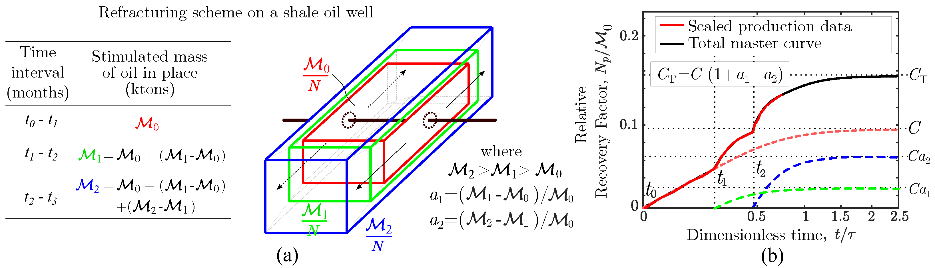
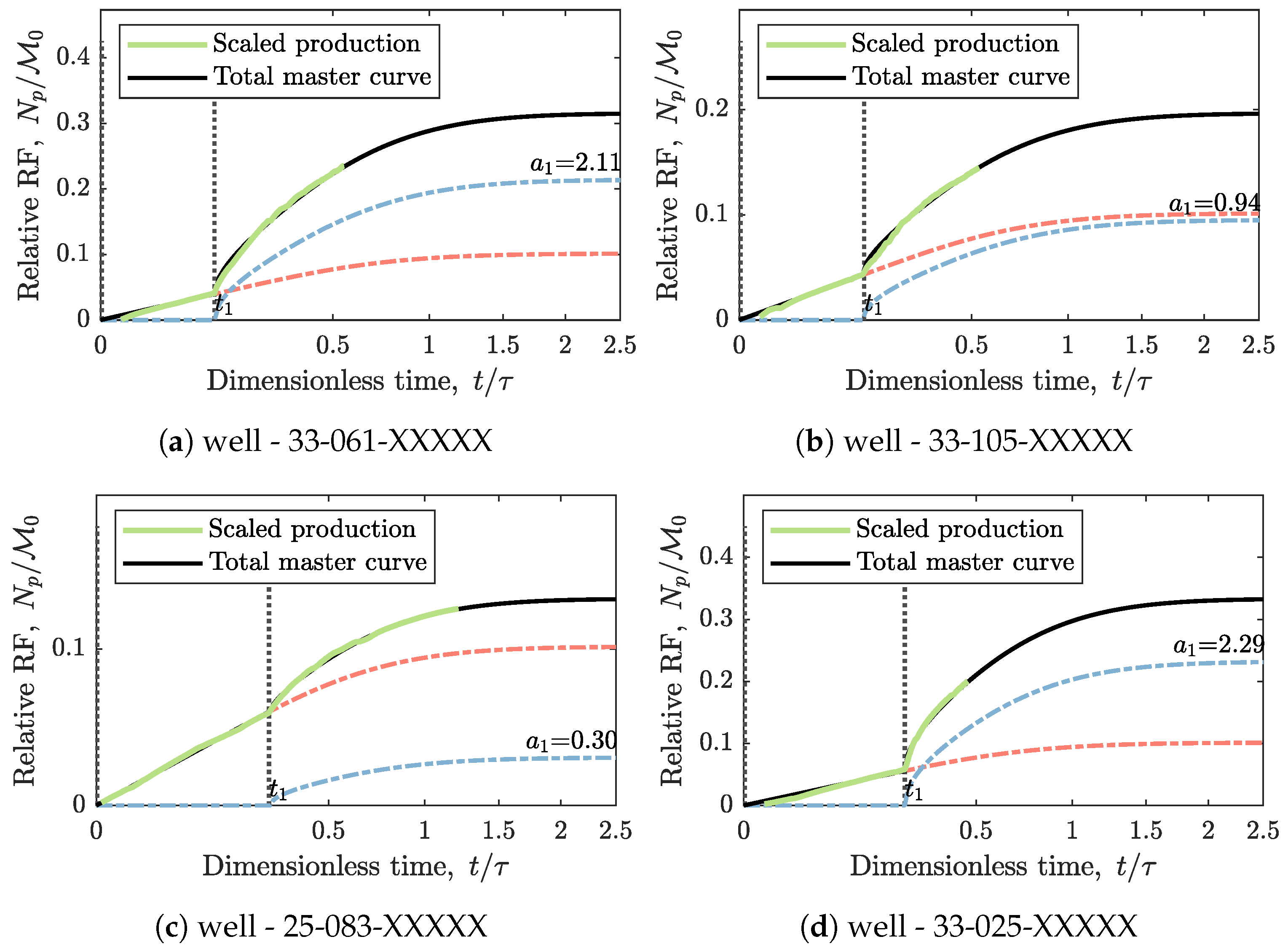
2.1.2. Physical Scaling of Well Refracturing

In many cases, the first hydraulic fracturing job is unsuccessful and results in a poor quality well that is a candidate for refracturing at a later time. Refracturing contributes to sudden jumps in production rate. The refracturing process is illustrated as an increase of the SRV in Figure 2a. As before, M is the initial mass of oil in place in the SRV. Before refracturing, the SRV box contains M 0 ktons of oil in place. At time t 1 , the first refracturing job is completed, and the mass in place jumps to M 1 . At t 2 , the second refracturing job is performed, and an even bigger M 2 is accessed. The refracturing process increases the mass M used to rescale cumulative oil production. By superposition theorem, this oil production is a summation of the production before refracturing that accessed the original mass in place, M 0 , and secondary production from imaginary wells at times t j , j = 1 , 2 , that access the incremental masses in place, ( M j M j 1 ).
min M > 0 , τ > 0 , a j 0 F ( M , τ , a j , ) = i = 1 t max [ ρ o , ST + R s ρ g , ST q o , ST ( t i ) Δ t i j = 0 n jump a j H j c t M 0 S o i ( p i p f ) 1 8 π 2 n = 0 1 ( 2 n + 1 ) 2 e ( ( 2 n + 1 ) 2 π 2 t i t j / ( 4 τ ) ) ] 2
The production jumps from refracturing cannot be scaled with the standard master curve shown in Figure 1. Thus, we combine the physical scaling solution with superposition and obtain Equation (12) that remedies this difficulty. If primary production before refracturing has the recovery constant C in Equation (13), then each refracturing event j at time t j activates an imaginary well with the recovery constant C a j . Here a j ’s are the new fitting parameters that scale effectiveness of each refracturing job relative to the initial mass in place, Equation (14). H j is the Heaviside step function that handles time delays in the consecutive refracturing jobs.
C = c t S o i ( p i p f )
a j = M j M j 1 M 0
H j = 0 , t i t j < 0 , 1 , t i t j 0 ,
The total master curve RF T is the summation of all individual master curves, RF j , see Equations (16) and (17). An example of matching the scaled discontinuous historical production is shown in Figure 2b.
RF T ( t ˜ ) = j = 0 n jump RF j ( t ˜ )
RF j ( t ˜ ) = a j H j C 1 8 π 2 n = 0 1 ( 2 n + 1 ) 2 e ( ( 2 n + 1 ) 2 π 2 t ˜ / 4 ) , where t ˜ = t i t j τ
Finally, one calculates EUR by multiplying the maximum total recovery factor from the modified master curve, RF T ( t ˜ max ) , with the initial mass of oil in place before fracturing, M 0 , Equation (18).
EUR T = RF T ( t ˜ max ) M 0 = C 1 + j = 1 n jump a j M 0

2.2. Data Collection and Scaling Procedure

We have mined public well records for the Bakken shale from the DrillingInfo (now Enverus) database, the Montana Department of Natural Resources and Conservation-Board of Oil and Gas Conservation website, and the North Dakota Department of Mineral Resources-Oil and Gas Division website with a premium subscription. In DrillingInfo, we have selected only 14,888 horizontal oil wells that were completed after 1 January 2000, in the Middle Bakken and Three Forks formations. The raw production data from DrillingInfo were imported into an integrated MATLAB ® software package we designed to perform data cleanup, consolidation, and unit conversions. The clean production data for each well consist of a vector of elapsed time on production (consecutive months with nonzero oil volume records) and a vector of cumulative oil production in kilotons.
Our scaling procedure of obtaining EUR for each well is as follows:
  • Exclude all newly completed wells with less than 12 months of production.
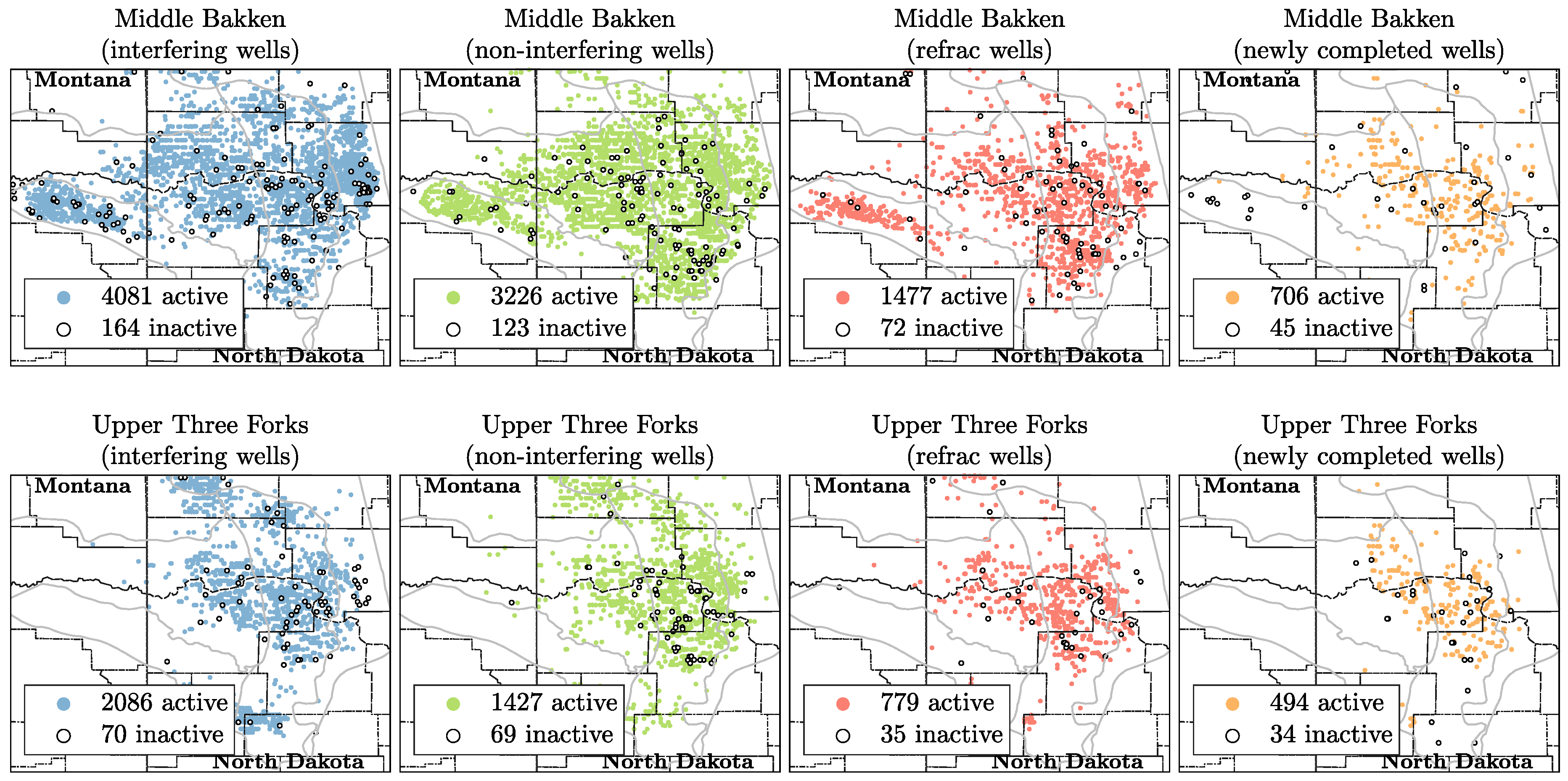
  • For each remaining well, plot its cumulative production vs. square root of time on production. Classify these wells as:
    (a)
    Non-interfering wells, if the plot shows a straight line (with, e.g., R 2 0.9 ).
    (b)
    Interfering wells, if the plot shows a deviation from a straight line (with, e.g., R 2 < 0.9 )
    (c)
    Refrac wells, if production jumps are detected.
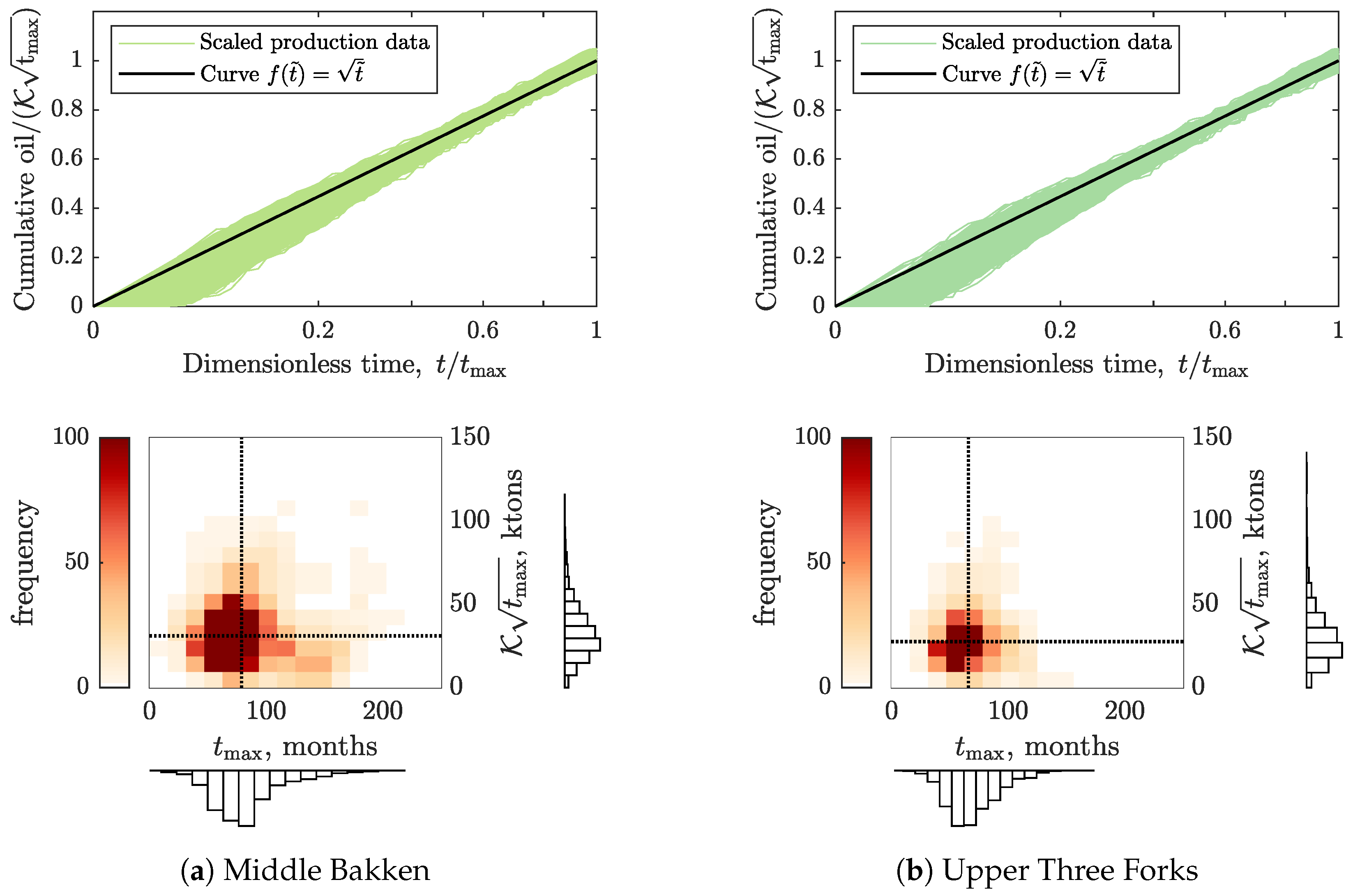
  • For each non-interfering well, scale its cumulative production by K t max , on the y axis and the elapsed time on production by t max on the x axis to match the line f ( t ˜ ) = t ˜ . To predict EUR, assume that deviation from the line starts at τ = 2 t max . Thus, the corresponding M can be calculated as M = ( K t max ) / RF ( 1 2 ) , where RF ( 1 2 ) is calculated from Equation (8). Finally, EUR is calculated from Equation (11).
  • For each interfering well, scale its cumulative production records to the master curve in Equation (8) using two scaling parameters, τ and M . The corresponding EURs are calculated from Equation (11).
  • For each refrac well, scale its cumulative production records to the master curve in Equation (16), and obtain optimum values of the scaling parameters τ , M 0 , and a j , j = 1 , 2 , . The corresponding EURs are calculated from Equation (18).
  • For each newly completed well, calculate its EUR using expected values of τ and M from comparable interfering wells that were completed between 2017 and 2019. Use Equation (11).
Notice that the EURs calculated from Equations (11) and (18) are in mass units. We use oil density to convert these EURs into thousands or millions of barrels (kbbl or Mbbl).

3. Results and Discussion

A quick scoping analysis shows the distribution of oil rates from all Bakken wells after—in this example—one year on production, see Figure 3. This distribution is positively skewed, meaning that most Bakken wells have low oil rates and the best wells with the significantly higher oil rates in the long tail are rare. The Generalized Extreme Value (GEV) distribution is most suitable to model the empirical oil rate distribution in the Bakken and other shales [27,33,34].
Using the GEV statistics of well populations, we calculate the high ( P 10 ), mean ( P 50 ), and low ( P 90 ), oil rate values from the cumulative distribution function (CDF). The P 50 well is the expected value of the distribution; the P 10 well is exceeded by only 10% of wells; and the P 90 well is exceeded by 90% of wells. Figure 4 shows the daily oil rates and cumulative oil production for all existing horizontal wells in the Middle Bakken and the Upper Three Forks. Notice that the Three Forks wells have fewer years on production because they were drilled after 2010. The P 10 , P 50 , and P 90 wells were calculated with the method discussed elsewhere [27,34] and in the caption of Figure 3. The expected ( P 50 ) maximum oil rate and cumulative oil are about 500 bbl/d and 200,000 bbl of oil for both Bakken and Three Forks.
In addition, many production jumps are observed. Each jump is a sudden discontinuity of oil rate that is sometimes larger than the initial oil rate in the same well, and an abrupt brake in cumulative production curve. These discontinuities may be caused by refracturing of old wells [35,36,37,38,39] or by changes of downhole well flowing pressure [40,41,42,43].

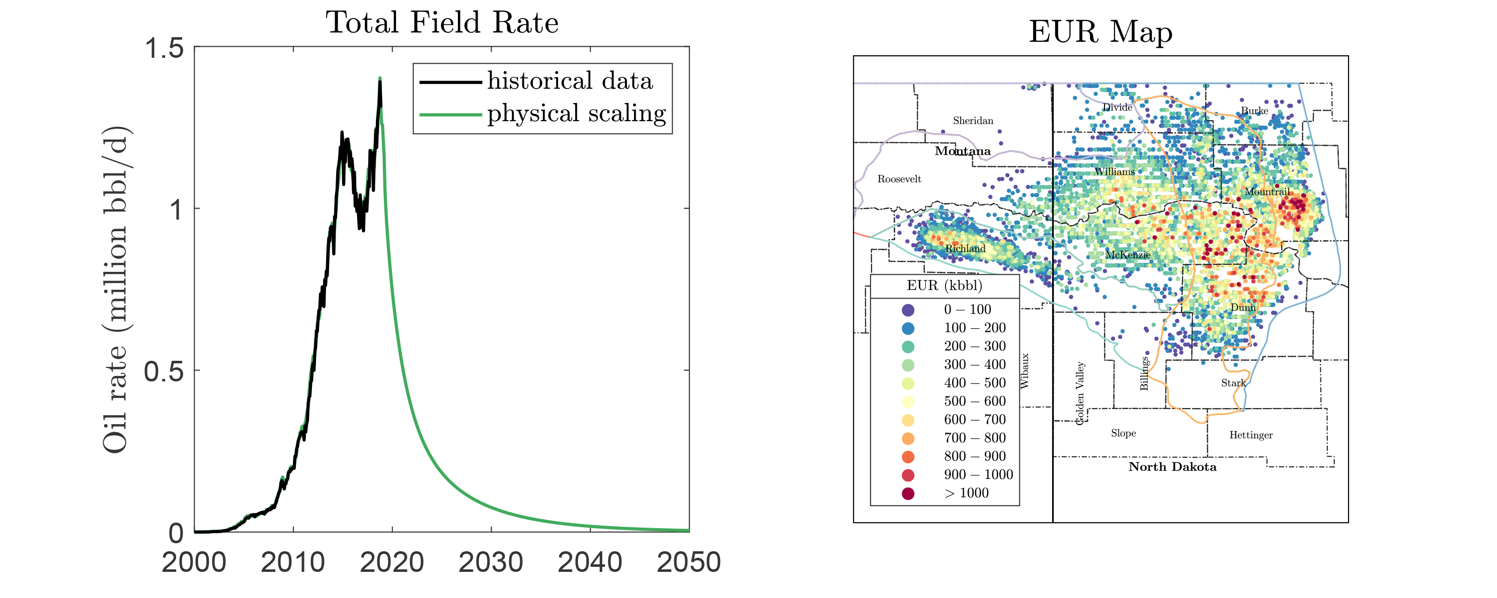
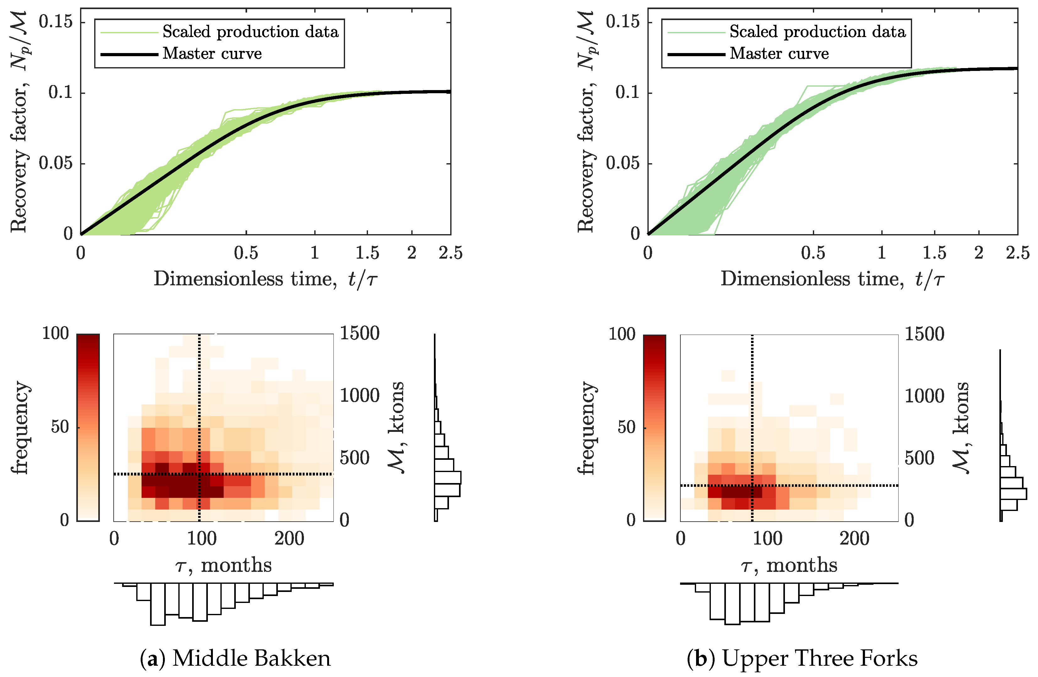
3.1. Physical Scaling Matches

We have scaled oil production from all 14,888 horizontal oil wells in the Bakken following the procedure detailed in Section 2.2. The reservoir properties used in scaling oil production are listed in Table A2. The key scaling results are shown in Figure 5, Figure 6 and Figure 7.
At the time of this analysis, 4845 Bakken wells, 3349 in the Middle Bakken and 1496 in the Upper Three Forks, were classified as non-interfering wells, because their cumulative production was still growing linearly versus the square root of time. The hyperbolic decline ( 1 / t ˜ ) of oil production rate from these wells is caused by the purely transient diffusion of oil pressure in the reservoir. Notice that the x-axis in Figure 5 is scaled with the maximum time on production, t max instead of τ and the y-axis is scaled with K t max to match the f ( t ˜ ) = t ˜ master curve that intersects point (1,1). In the Middle Bakken, the expected values of t max and K t max are 75 months and 30 ktons, respectively, while in Three Forks these values are 65 months and 27 ktons. For the non-interfering wells, we assume arbitrarily that they start to decline exponentially (go under the square-root-of-time linear trend) at τ = 2 × t max .
The interfering wells exhibit clear pressure interference between consecutive hydrofractures and are in pseudo-steady state flow regime. For each well k, this interference already occurred at the elapsed time on production t = τ k and, at the time of this analysis, each oil production rate was declining exponentially. For these wells, the recovery factors start bending down at the dimensionless time equal 0.5 < 0.64 in [24] because oil is less compressible than gas. The interfering wells scale with the master curve in Figure 1. Of the 6401 interfering wells in the Bakken, 4245 were in the Middle Bakken and 2156 in the Upper Three Forks (Figure 6). The expected values of τ and M were 100 months and 420 ktons for the Middle Bakken, and 90 months and 320 ktons for the Upper Three Forks.
Many wells in the Bakken (2363) cannot be scaled to a non-interfering or interfering segment of the scaling curve. The poor matches are caused by multiple production jumps that may be due to refracturing of old wells [35,36,37,38,39]. We note that these jumps could also result from artificial lift and step decreases of downhole well pressure [40,41,42,43]. Each of these wells is scaled individually with a modification of the full physical scaling curve coupled with superposition (illustrated in Figure 2). Four examples of “refrac wells” are shown in Figure 7. The wells in panels a and c have been completed in the Middle Bakken formation, while the those in panels b and d in the Upper Three Forks formation. As we can see, the modified scaling curve matches the discontinuous production records. The magnitude of each a in Equation (14) may reflect effectiveness of a specific refracturing job. For all “refrac wells,” the expected value of a is about 0.6, a little better than 50%.
The remaining 1279 newly completed wells had less than 12 months on production at the time of this analysis. The oil production rates from these wells are usually unstable due to backflow of fracturing fluids, excessive choking and/or lack of takeaway capacity [24,25,44,45,46,47,48].
During the first three months on production in each well, the produced cumulative oil volume is commonly below the square-root-of-time line due to the unloading of SRV from fracturing fluids, whose flow blocks oil production, [24,25]. If a well does not have enough of stable production history, its scaling will underestimate both τ and M . Therefore, we have decided to use the average τ and M values from scaling the recently completed (in 2017–2018) interfering wells with τ = 45 months and M = 495 ktons for the Middle Bakken and 43 months and 390 ktons for the Upper Three Forks. Notice that the magnitude of τ is lower and that of M is higher for the new wells. These shifts are caused by the improvements of well completion technology over the last decade [49,50,51,52,53,54,55], i.e., by bigger hydrofractures, fewer clusters per stage, more fracture stages, etc.
Table A3 details the interference times, τ , and the masses of oil in place, M , for the four well classes: (1) interfering, (2) non-interfering, (3) refracs, and (4) newly completed wells in the Middle Bakken and Upper Three Forks. The surface location maps of these four well classes are shown in Figure 8 for both reservoirs. For the Middle Bakken, wells in the first three classes spread extensively from the center of the Williston Basin in North Dakota to the Elm Coulee Field in Montana, while in the Three Forks few wells were drilled in Montana. Interestingly, the newly completed wells are located mostly in the central part of the Williston Basin in North Dakota. There were some new wells completed in Montana; however, they became inactive within the first few months on production. In general, the magnitudes of τ and M in the Upper Three Forks are lower than those in the Middle Bakken, indicating that the Three Forks wells decline faster and have lower EURs than those in the Middle Bakken. The refrac wells have the highest values of M , because of the incremental stimulated reservoir volumes due to refracs. The non-interfering wells have slightly higher EURs than the interfering wells, because of the larger τ and M values. As mentioned before, the newly completed wells have shorter τ s and larger M s than all other well classes. Each of these wells starts from a very high initial production rate that declines very fast.

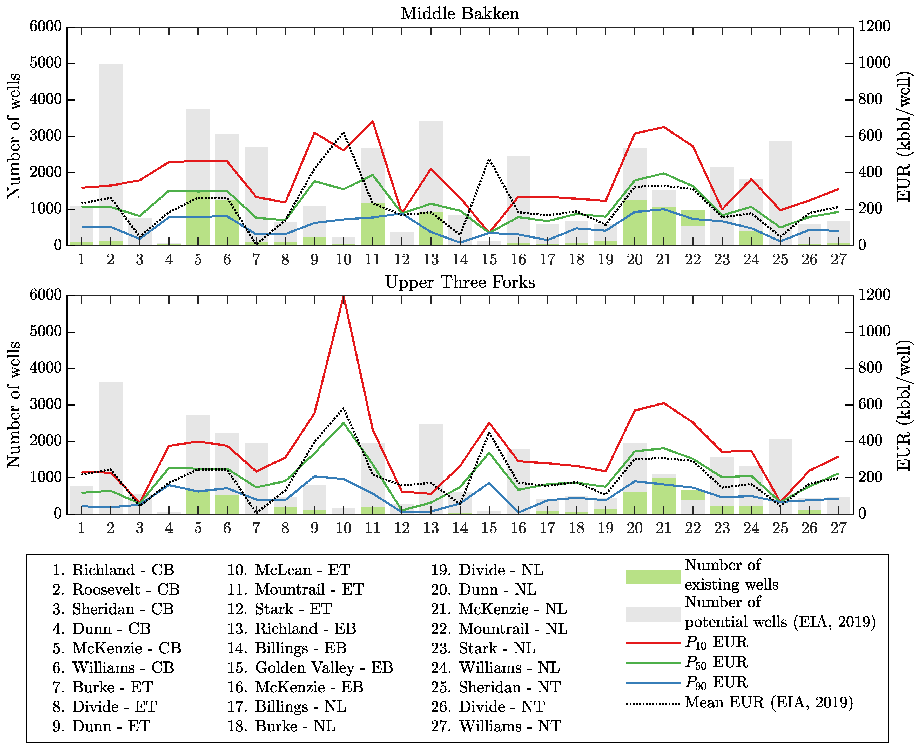
3.2. EUR Predictions

To predict the fieldwide EUR, all individual scaling curves for the 14,888 existing wells in the Bakken are summed up vs. calendar time (Figure 9). For each well class, we note the high fidelity of the physical scaling approach in retracing old production and—by implication—forecasting future production of the existing wells. From Figure 9 (left), we infer that the second production peak in the last three years is not only the contribution from the newly completed wells that are highly productive, but also from the old wells that have been refractured or pumped off recently. From Figure 9 (right), it follows that the expected estimated ultimate recovery from all 14,888 wells in the Bakken play is about 715 million m 3 (4.5 billion bbl) of oil. The EURs for the interfering and non-interfering well classes are almost the same at about 240 million m 3 (1.5 billion bbl) each, as the respective well numbers are close: 6401 and 4845. The refrac wells have a larger average EUR per well with total EUR of 160 million m 3 (1 billion bbl) from only 2363 wells. The recent 1279 wells also have a higher EUR per well with the total EUR of 80 million m 3 (0.5 billion bbl). One can argue that success of the newly completed wells in yielding the highest EURs is not only due to the significant improvements in well completion techniques, but also to the favorable drilling location selections across the most prolific area in the Bakken, near the center of the Williston Basin (recall Figure 8).
Figure 10 shows that our physical scaling method and the hyperbolic decline curve analysis (DCA) give different estimates of oil production from the Bakken shale. To solve for the matching parameters of hyperbolic DCA, initial oil rate, q i ; initial decline rate, D i ; and the hyperbolic exponent, b, we used the algorithm described in the Reservoir Engineering Handbook (Fourth Edition) by Tarek Ahmed [56]. In addition, we wrote a MATLAB® program to automate the hyperbolic DCA matches of 14,888 Bakken oil wells. Figure 10a,b are examples of the respective matches of oil production from well -25-083-XXXXX. The rate is plotted on a semilog scale and there seem to be no large discrepancies between the physical scaling (blue curve) and hyperbolic DCA (red curve) matches of the past oil rate (black line). However, when we integrate the rate estimates from both methods to obtain cumulative production, the hyperbolic DCA fails to trace past production and gives an overly optimistic cumulative oil of 64,000 m 3 (400 kbbl) at the last production time recorded. In contrast, the physical scaling yields 55,600 m 3 (350 kbbl) matching exactly historical data. We also quality-checked both methods for 11,246 non-refractured wells in the Bakken, see Figure 10c,d. For each well, each point in these cross-plots quantifies agreement between the actual annual rate (the volume of oil produced during 12 months on production in kbbl/year), in year 1 , 2 , , and the corresponding values predicted with both methods. There are 61,230 points in each of the two cross-plots. Ideally, these points would follow the diagonal line, y = x . For DCA, best data fit, y = 1.12 x + 1.14 , (the blue line) is biased towards excessive predicted production volumes. The linear model explains the data almost perfectly and its 95% confidence interval (CI) is not plotted. The two dashed blue lines denote the 95% CI band that a new data point in the same set of wells would fall inside of this band. The physical scaling model is not biased, y = 0.99 x 0.13 , and its 95% CI is narrower. Finally, we stacked up all rate estimates from the 14,888 oil wells in the Bakken to obtain total field rate shown in Figure 10e. At the field scale, the systematic upward bias of hyperbolic DCA is amplified, thus, the red line fails to track the black line. In contrast, the stack of individual physical scaling matches (blue line) traces historical production. The total field cumulative is shown in Figure 10f. In the end, there is a big discrepancy between both methods of predicting total field EUR from the same field production data set. The physical scaling predicts the EUR from the 14,888 existing wells at 715 million m 3 (4.5 billion bbl), while the hyperbolic DCA is overly optimistic, giving a 45% higher estimate of 1 billion m 3 (6.5 billion bbl).
The current model is a mechanistic scaling of well production in the Bakken shale based on the first order physics of production mechanisms in hydrofractured horizontal wells and on geology. It served as the physical foundation of the statistical prediction [34] of ultimate production in the Bakken based on the Generalized Extreme Value (GEV) statistics. The current scaling model provides an unbiased match of all historical data from all wells in the Bakken. The width of the 95% CI in Figure 10d reflects the natural variability of reservoir and well properties that influence the model predictions around their expected values listed in Table A2. The 61,230 points that make the comparison in Figure 10d demonstrate that the stochastic variability of reservoir and well properties is rather small and the model does an excellent job finding the unbiased values of original oil in place M and pressure interference time τ for each of the 14,888 wells in the Bakken.
To compare our results with EUR predictions from the US DOE Energy Information Administration [6], we have remapped each Bakken assessment unit onto counties and calculated the expected value of EUR for each county. The details are tabulated in Table A4. We predict the EUR from all 14,888 active horizontal oil wells in the Bakken to be 715 million m 3 (4.5 billion barrels of oil) or ∼48 thousand m 3 /well (300 kbbl/well), with 493 million m 3 (3.1 billion barrels) coming from 9894 wells in the Middle Bakken and 222 million m 3 (1.4 billion bbl) coming from 4994 wells in the Upper Three Forks. The results in Table A4 are also displayed as stacked bar graphs for the Middle Bakken and the Upper Three Forks (Figure 11). The stacked bars show the numbers of existing wells from the DrillingInfo dataset in 2019, and the potential wells from [6] in each Bakken Total Petroleum System (TPS) assessment unit mapped onto the corresponding counties in the Middle Bakken and Upper Three Forks Formations. The lines show the corresponding EUR values from the physical scaling and the EIA statistical predictions. The P 10 , P 50 , and P 90 wells were obtained by applying the generalized extreme value (GEV) distribution [27,34] for each set of EURs from the scaling curve method in each sub-region as demonstrated before in Figure 3.
In most cases, where there are enough wells per sample, the expected P 50 EURs from physical scaling agree with the EUR estimates by EIA. One can observe that most of the best regions with the high EUR values have been extensively drilled leaving no or few potential wells to infill. Mountrail-NL is an extreme example of over-drilling in the best region of the Bakken, where the number of existing wells exceeds the number of EIA potential wells by 40% (the green bar is taller than the gray bar). In another paper [34], we have calculated well density of all regions in the Bakken, revealing a surprising result that the core area of the Bakken will be fully drilled by 2021. In contrast, most of the 85,334 potential wells proposed by EIA will be in the poorest regions of the Bakken. Figure 12 maps the EUR results from physical scaling approach for 14,888 horizontal oil wells in the Bakken. Notice that this map resembles more the water cut map (Figure A3), rather than the GOR map (Figure A3).
In Figure 13a, we show that EUR is negatively correlated with water cut ( 1 oil cut ). On the other hand, there is little correlation between EUR and lateral length, as depicted in Figure 13b. Doubling lateral length from 1.5 to 3 km (5000 to 10,000 ft) does not double average EUR that increases from 38 to 49 thousands of m 3 (240 to 310 kbbl). This finding may also suggest that better technology cannot increase EUR if a well is drilled in a low-productivity region of the Bakken.
Figure 14 shows the average values of pressure interference time, τ , lateral length, gas–oil ratio, and water cut for each six-month time interval in calendar dates. The value of τ decreases significantly over time meaning that newer wells pressure-interfere and decline faster than the old ones. Equation (7) shows that τ is directly proportional to the square of half-distance, d, between two consecutive hydrofractures. This means that halving the interfracture distance decreases τ four-fold. Historically, the number of hydrofracture stages in the Bakken has increased over time from 8 stages in 2007 [52], to 18 stages in 2009 [53], 35 stages in 2016 [54], and to as many as 60 stages in 2019 [55]. The lateral length has also doubled from 1.5 km (5000 ft) in 2005 to 3 km (10,000 ft) in 2015.
In summary, the new completion techniques in the Bakken shale rely on more of bigger hydraulic fractures and on longer laterals [49,50,51]. These new completions have significant side-effects. Cumulative gas–oil ratio has been increasing in both the Middle Bakken and Three Forks. The likely culprits are reservoir depressuring by hydrofractures that are too close and the increasingly aggressive artificial lift. Degassing the low permeability and porosity reservoirs in the Bakken spells trouble for future production, because solution- and free gas are the main driving mechanisms of primary depletion. Water cut has also increased with time revealing another negative side-effect of the recent Bakken field development. The increasing water cut might be caused by drilling new low-productivity wells in the immature regions of Bakken [57,58,59], and/or by the longer and taller hydraulic fractures that break into adjacent water-bearing formations, the Lodgepole and/or Lower Three Forks [60,61,62].

4. Conclusions

We have delivered a comprehensive physics-based scaling of all horizontal hydrofractured wells completed in the Middle Bakken and Upper Three Forks between 1 January 2000, and 1 May 2019. In particular:
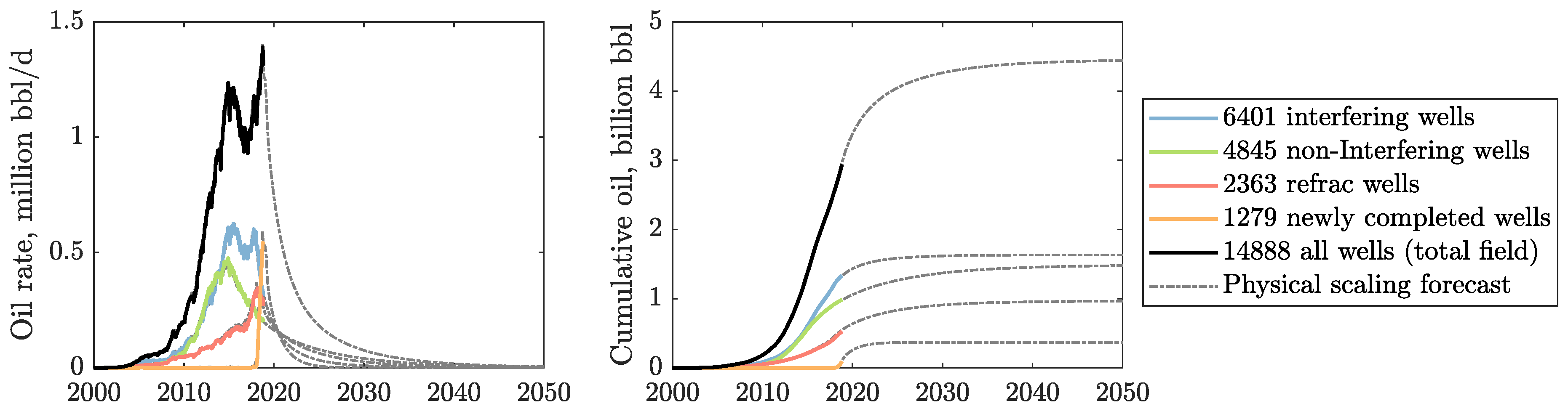
  • The current 14,888 active oil wells in the Bakken shale will ultimately produce 715 million m 3 (4.5 billion barrels) of oil, with 493 million m 3 (3.1 billion barrels) from 9894 wells in the Middle Bakken and 222 million m 3 (1.4 billion barrels) from 4994 wells in the Upper Three Forks.
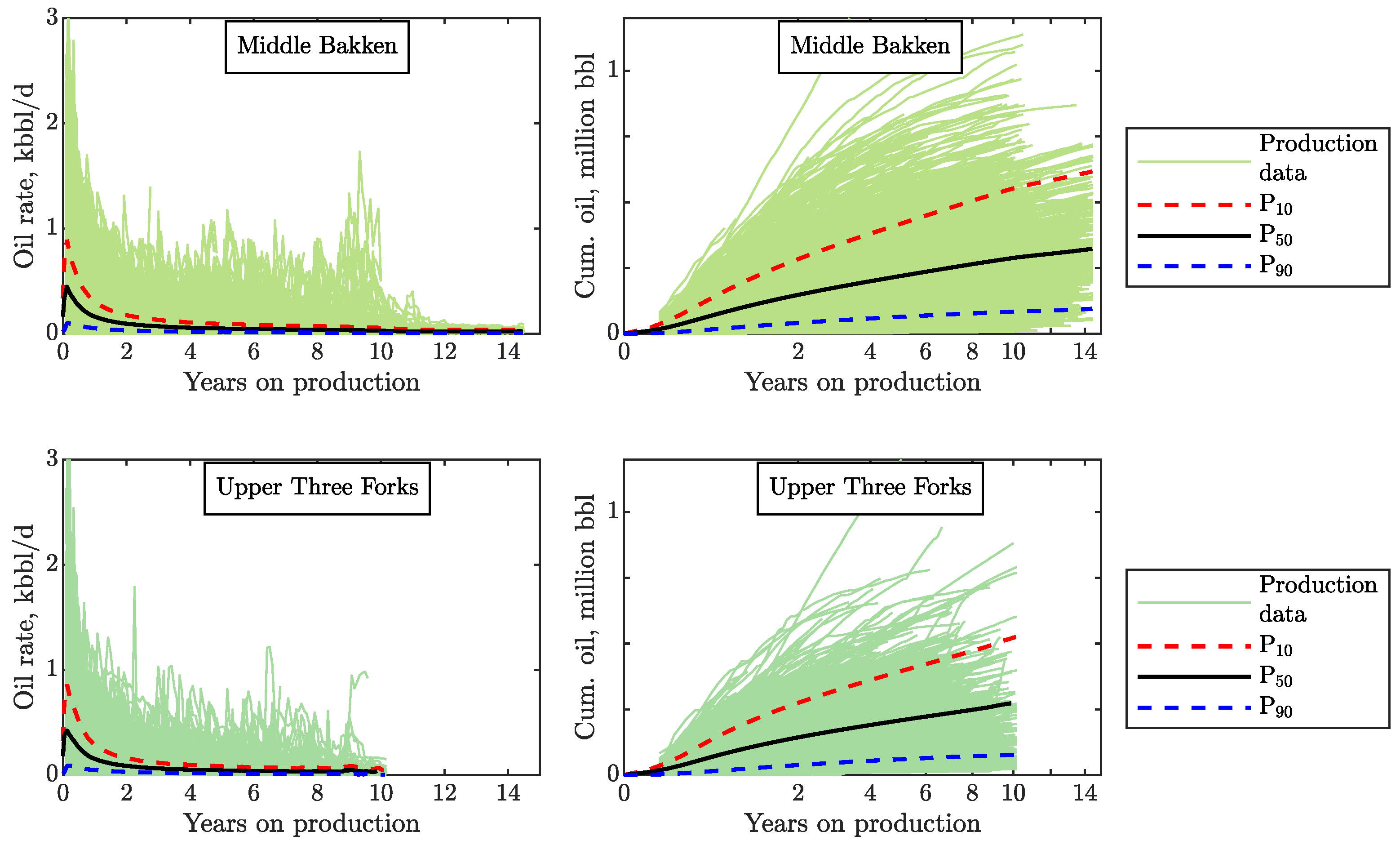
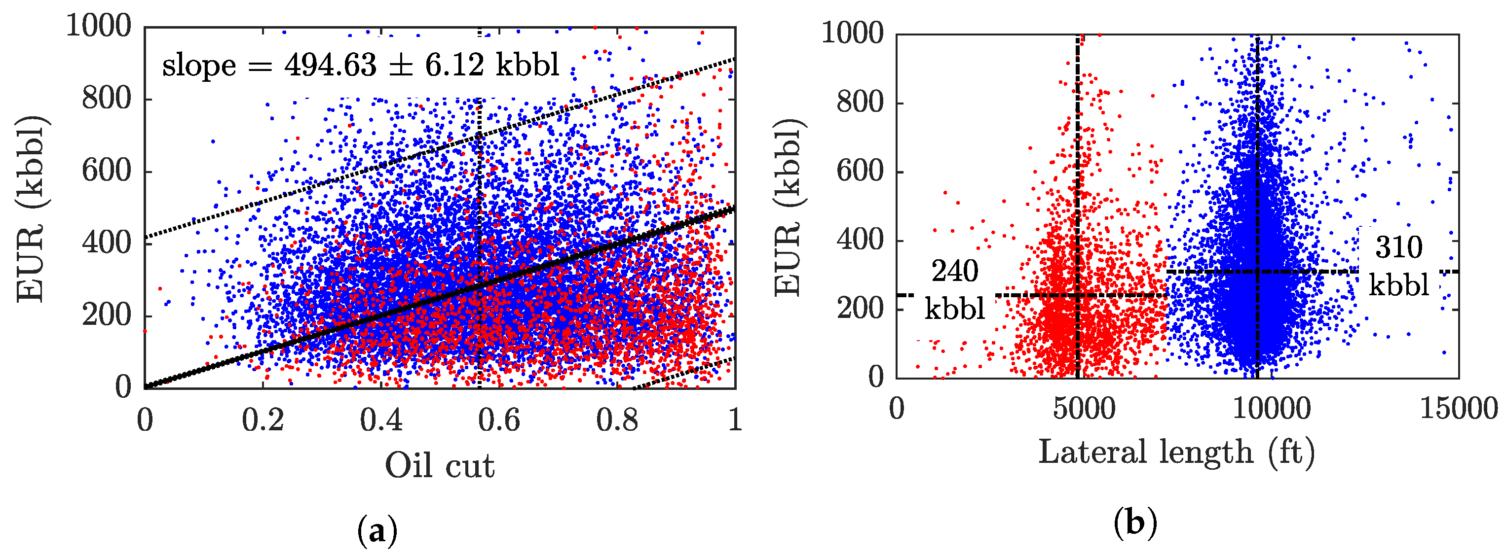
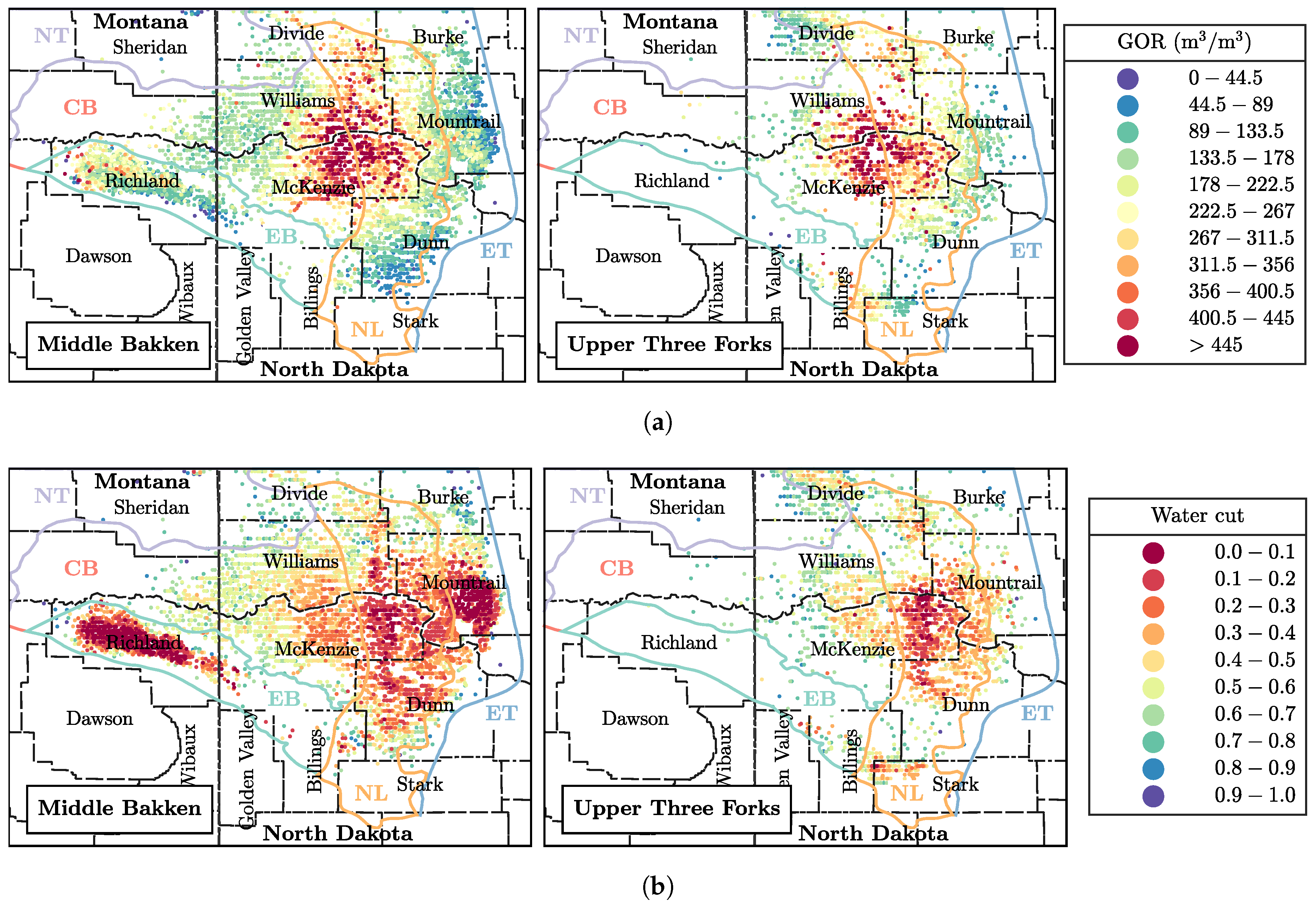
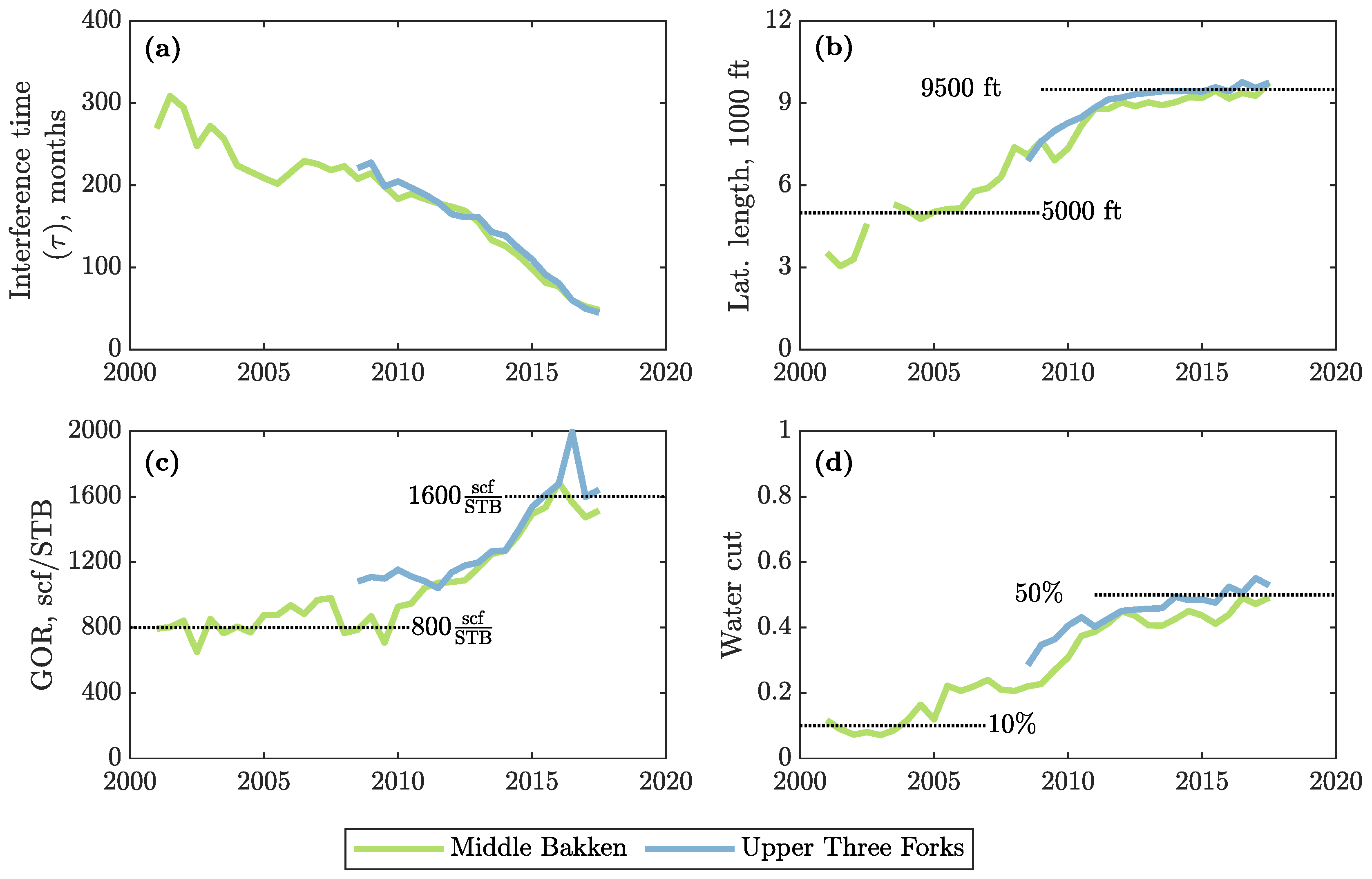
  • In general, wells completed in the Middle Bakken produce more oil than those in the Upper Three Forks due to: (1) lower water saturation and water cut, (2) slower decline rate (longer pressure interference times, τ ), and (3) higher initial oil in place (larger M ).
  • Newly completed wells start from very high initial oil rates but in general decline faster than the pre-2010 wells. Still, we predict higher EURs for the newly completed wells.
  • The more productive newer wells result from recent advancements in completion technology: longer laterals, larger hydrofractures, bigger stimulated reservoir volumes, and more fracture stages.
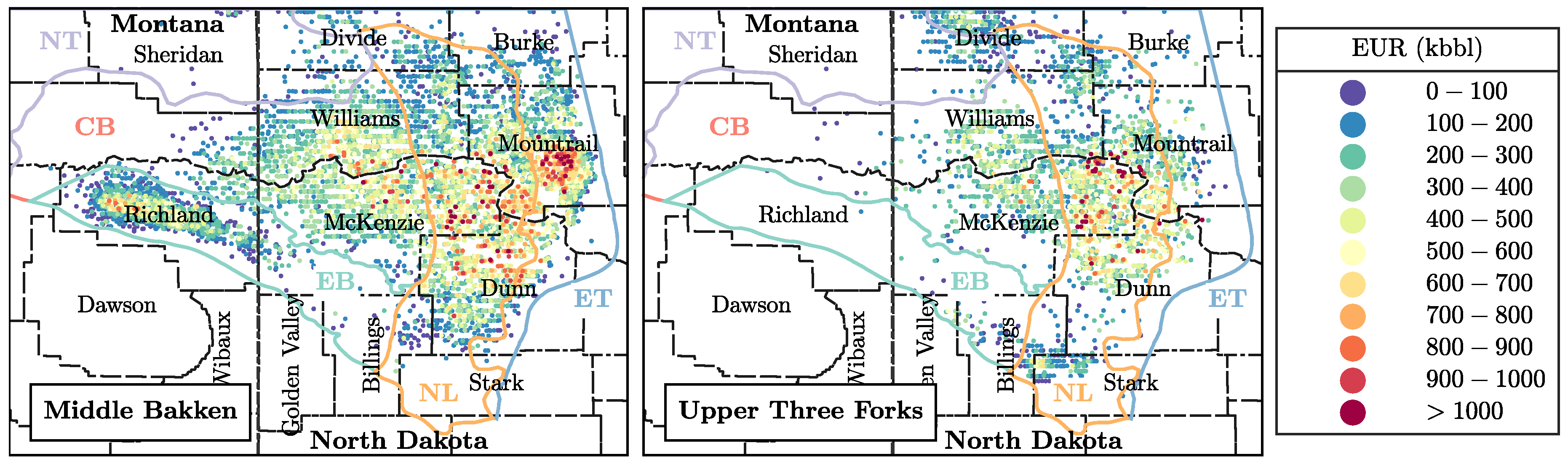
  • Operators have also learned to drill new wells only in the most prolific area of the Bakken region at the center of the Williston Basin.
  • With time, negative trends in oil production have amplified in the Bakken. We observe higher GOR values (reservoir degassing); higher water cuts (contacting water-bearing formations and drilling in regions with lower oil saturations); faster decline rates; and excessive well density, especially in the most prolific areas.
  • When all most productive areas in the Bakken are extensively drilled, the poor immature areas with high water production will be the only targets left for infill drilling. In this case, technology will not enhance much performance of the future wells.
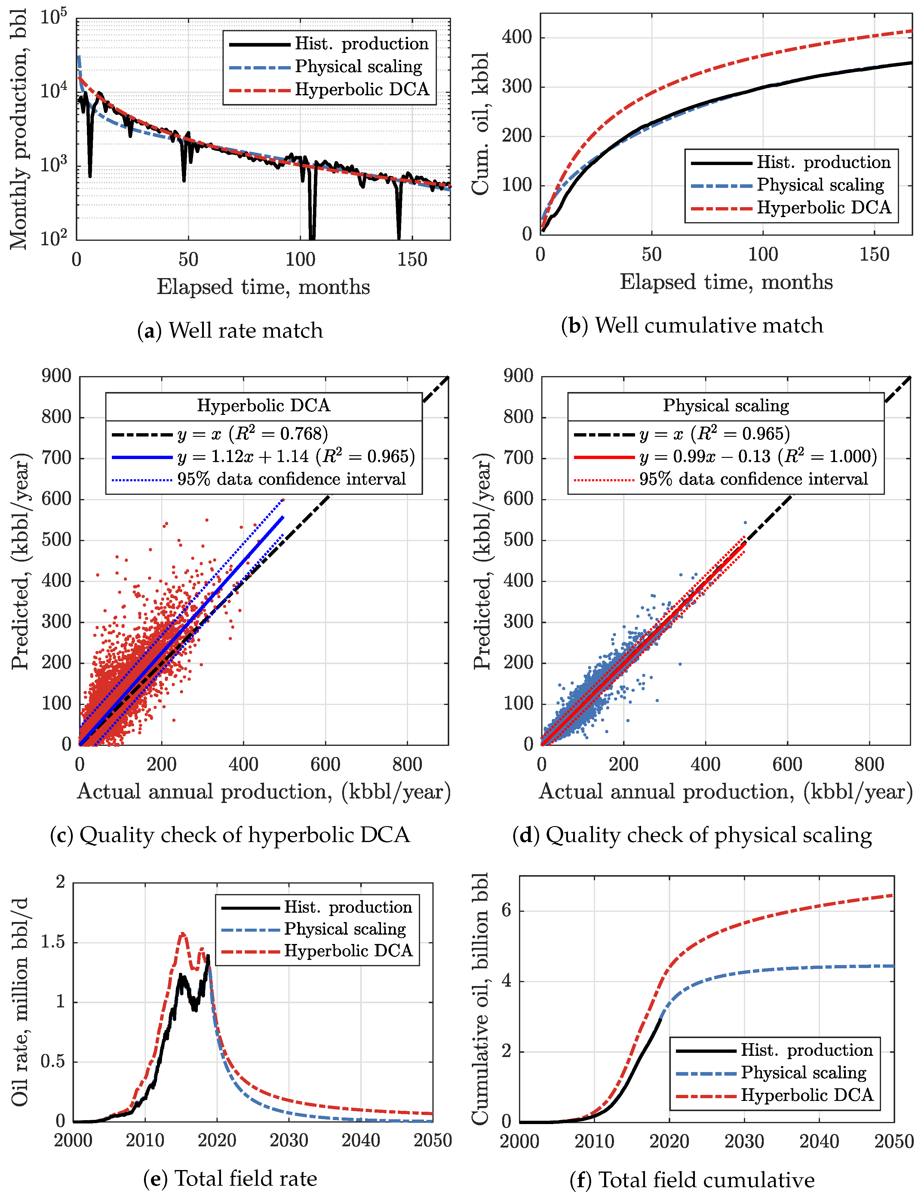
  • We encourage practitioners to adopt our fast and accurate method of predicting oil production in shales that is a viable alternative to the hyperbolic DCA which yields an ‘illusory picture’ of shale oil resources.
Elsewhere [34], we have outlined a hybrid method that combines the precise GEV statistics of horizontal oil wells in the Bakken with the physics-based scaling method developed in this paper and combined with late-time inflow [26]. This hybrid approach follows from our comprehensive evaluation of the Barnett play futures [27].

Author Contributions

Conceptualization, T.P. and W.S.; methodology, T.P. and W.S.; software, W.S. and T.P.; validation, T.P. and W.S.; formal analysis, W.S. and W.K.; investigation, W.K. and W.S.; resources, T.P.; data curation, W.K.; writing–original draft preparation, W.S.; rewriting manuscript–review and editing, T.P. and W.S.; visualization, W.S.; supervision, T.P. and W.K.; project administration, T.P.; funding acquisition, T.P. All authors have read and agreed to the published version of the manuscript.

Funding

Wardana Saputra (PhD student) was supported by baseline research funding from KAUST to Tad Patzek. Wissem Kirati (Research Engineer) was supported by the Division of Computer, Electrical and Mathematical Science at KAUST.

Acknowledgments

The authors thank the Ali I. Al-Naimi Petroleum Engineering Research Center (ANPERC) at KAUST for supporting this research. We thank the reviewers for their thorough, informative and timely reviews.

Conflicts of Interest

The authors declare no conflict of interest.

Nomenclature

a j effectiveness of a refrac job
A f one-sided area of hydrofracture, ft 2 [m 2 ]
c o oil compressibility, psi 1 [Mpa 1 ]
c w water compressibility, psi 1 [Mpa 1 ]
c ϕ pore space compressibility, psi 1 [Mpa 1 ]
c t total compressibility, psi 1 [Mpa 1 ]
Cmaximum recovery factor before refracturing, fraction
dhalf-distance between two consecutive hydrofractures, ft [m]
EUR estimated ultimate recovery of oil, million bbl, Mbbl
EUR T total estimated ultimate recovery of oil from a refractured well, million bbl, Mbbl
GOR dissolved gas–oil ratio, scf/stb [sm 3 /m 3 ]
Hfracture height, assumed equal to formation thickness, ft [m]
H j Heaviside unit step function
ithe i t h month on production
jthe j t h discontinuity of production rate from a refracturing event
kaverage permeability of the matrix, μ d [m 2 ]
K dimensional scaling constant, kton/ month
Lhydrofracture half-length, ft [m]
M mass of saturated oil inside stimulated reservoir volume, kton
M 0 mass of saturated oil inside stimulated reservoir volume before refracturing, kton
M j mass of saturated oil inside stimulated reservoir volume after jth refracturing, kton
Ntotal number of parallel vertical hydrofractures in a well
N p cumulative mass production of oil, kton
ppressure, psi [Mpa]
p i estimated initial formation pressure, psi [Mpa]
p b average bubble point pressure, psi [Mpa]
p f constant pressure in hydrofractures, psi [Mpa]
P x a number such that there is an x % likelihood that true value exceeds P x
qoil production rate at downhole conditions, bbl/day [m 3 /s]
q S T oil production rate at stock tank conditions, bbl/day [m 3 /s]
R 2 a statistical measure of how close the data are to the fitted regression curve
q field , ST volume of oil produced in month i by a horizontal well, stb/month
RF recovery factor, fraction
RF j recovery factor for an imaginary well due to jth refracturing event, fraction
RF T total recovery factor for a refractured well, fraction
R s solution gas–oil ratio, scf/stb [sm 3 /m 3 ]
S o i initial oil saturation
S w c connate water saturation
telapsed time on production, months [s]
t j elapsed time when jth refracturing event occurs, months [s]
t ˜ dimensionless time
xdistance, ft [m]
α pressure diffusivity coefficient, m 2 /s
α i pressure diffusivity coefficient at initial conditions, m 2 /s
β exponent constant in simplified master curve equation
λ Conway’s constant ≈ 1.30357
μ o oil viscosity, cp [Pa s]
μ o i oil viscosity at initial conditions, cp [Pa s]
ρ fluid , i fluid density at initial conditions, lb/ft 3 [kg/m 3 ]
ρ g , ST gas density at stock tank conditions, lb/ft 3 [kg/m 3 ]
ρ o oil density, lb/ft 3 [kg/m 3 ]
ρ o i oil density at initial conditions, lb/ft 3 [kg/m 3 ]
ρ ST oil density at stock tank (dead oil) conditions, lb/ft 3 [kg/m 3 ]
ρ w water density, lb/ft 3 [kg/m 3 ]
ϕ porosity, fraction
τ characteristic pressure interference time, months

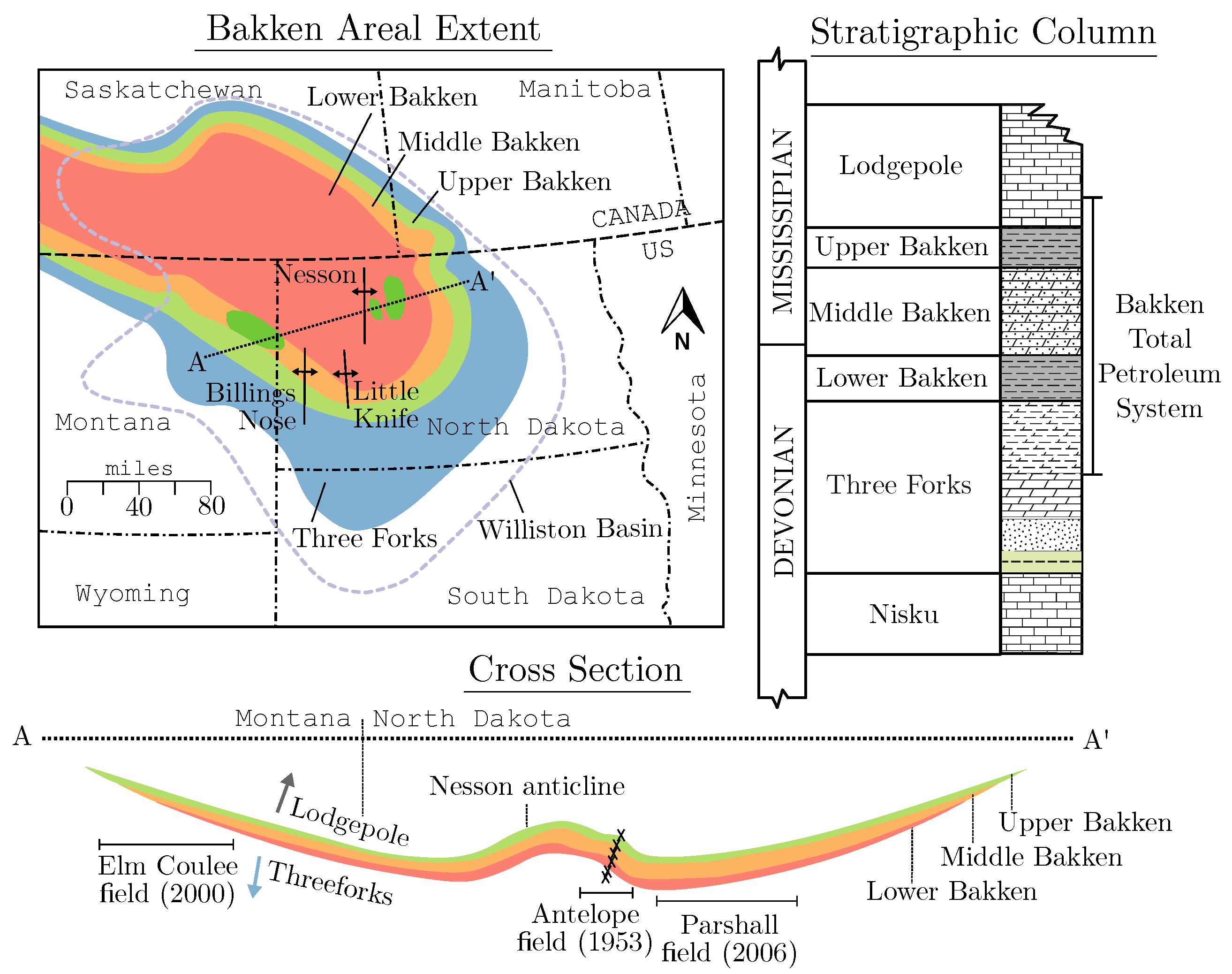
Appendix A. Overview of the Bakken Shale Play
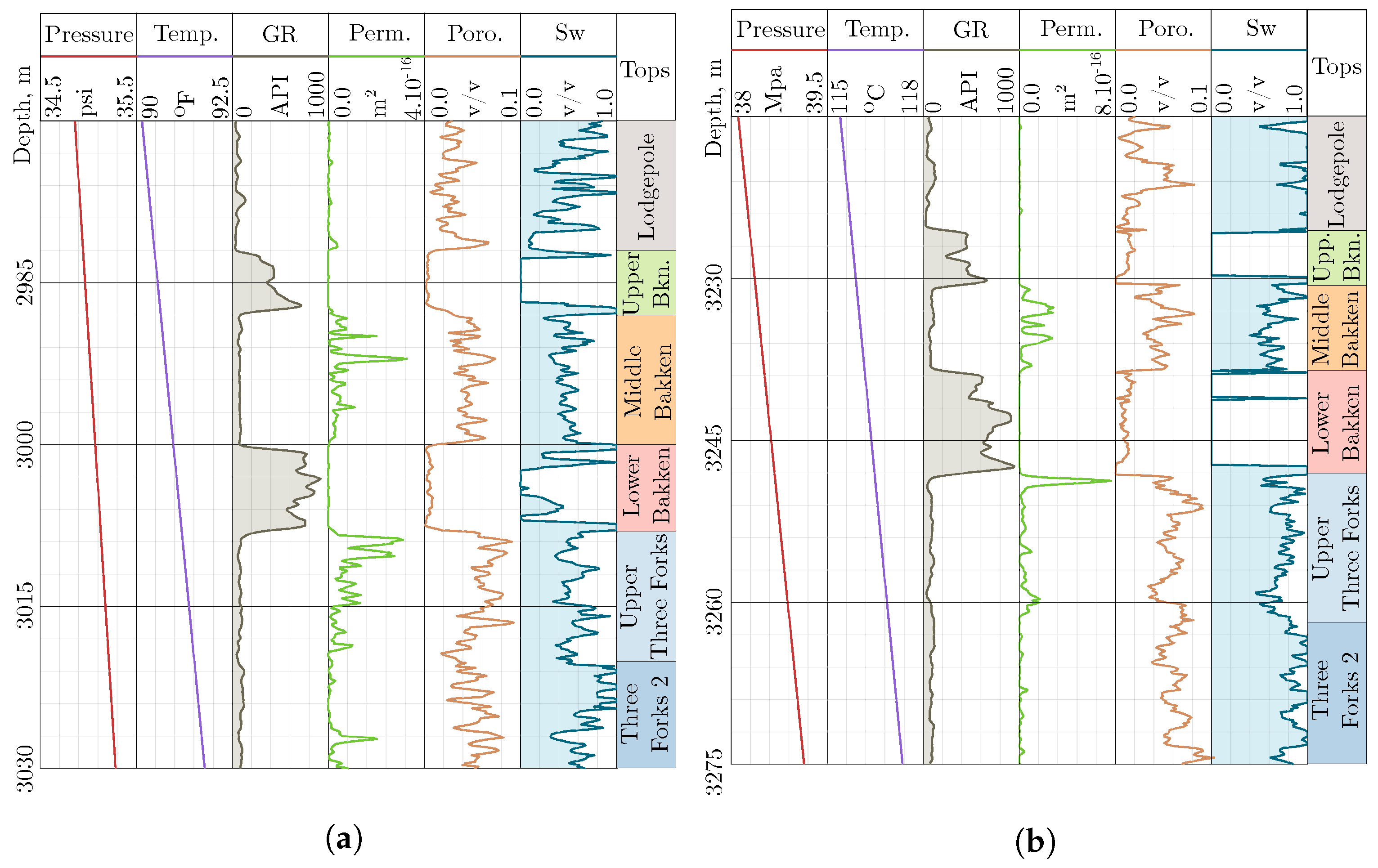
The Bakken mudrock play was discovered in 1953, in the Antelope Field, North Dakota, with the completion of the #1 Woodrow Starr well by Stanolind O&G Corp. [63]. Outside of Antelope field, the Bakken formation was not considered to be economically viable because it was generally impermeable [63,64]. The success of old vertical wells drilled in the Antelope Field depended upon naturals in the Bakken and Three Forks (Sanish) Formations [64].
The Bakken was not developed until the early 2000s, when about 20,000 barrels of oil per day were produced from the Elm Coulee field in Montana. Improvements of horizontal drilling techniques and advancements in hydraulic fracturing enabled massive drilling in the Bakken in the past ten years. By 2014, more than 10,000 horizontal wells were drilled in 14 counties in Montana and North Dakota, leading to the first production peak in the Bakken at 0.19 million m 3 /day (1.22 Mbopd). In early 2019, Bakken ranked as the second largest oil producer in the US, with the second major oil peak of 0.23 million m 3 /day (1.45 Mbopd) from 14,888 horizontal, hydrofractured oil wells. The predicted technically recoverable oil in the Bakken region is about 1.18 billion m 3 (7.38 billion barrels) of oil according to the US Geological Survey [4], and 15.6 billion barrels of oil according to the US DOE Energy Information Administration [6].
Figure A1. Areal extent, stratigraphic column, and cross-section of the Bakken Total Petroleum System (TPS), modified from [4,57,58].
Energies 13 02052 g0a1
The areal extent, cross-section, and the stratigraphic column in the Bakken are shown in Figure A1. The Bakken total petroleum system (TPS) lies on a bowl-like intracratonic Williston Basin, which covers an area of 200,000 square miles (518,000 km 2 ) across parts of North Dakota and Montana in the US, and into the Saskatchewan Province in Canada. The Bakken TPS is a continuous petroleum system that consists of three Bakken members, the Upper Three Forks and the Lower Lodgepole [4]. The Upper Bakken and the Lower Bakken are world class shale formations with total organic carbon (TOC) of about 10%. These formations are the source of hydrocarbons in the dolomitic Upper Three Forks and silty dolomitic Middle Bakken members. The Middle Bakken and Upper Three Forks formations are the two major drilling targets for recent field developments.
The average reservoir properties of the three Bakken members and the Upper Three Forks were derived from well log data in McKenzie and McLean counties, North Dakota, (Figure A2), and are summarized in Table A1.
The average formation depth of all layers is about 3108 m (10,120 ft). At this depth, the initial formation pressure and temperature are about 37 Mpa (5300 psia) and 105 ° C (220 ° F), respectively. Because the Upper and Lower Bakken formations are shales, the gamma-ray log readings there are as high as 690 ° API and the permeability is as low as 2 × 10 19 m 2 (200 nanodarcy). The main drilling targets, Middle Bakken and Upper Three Forks, have a better permeability of about 5 × 10 17 m 2 (45 microdarcy). The Upper Three Forks formation has a slightly higher porosity and thickness than those in the Middle Bakken, but it also has a higher water saturation, indicating that the Three Forks wells must produce more water.
Figure A2. Bakken well log data of well-33-055-XXXXX (a) and well-33-053-XXXXX (b) from the North Dakota Department of Mineral Resources—Oil and Gas Division home page.
Energies 13 02052 g0a2
Table A1. The average reservoir properties from well log data shown in Figure A2.
FormationUpper BakkenMiddle BakkenLower BakkenUpper Three Forks
Depth (m)3108311631253136
Pressure (Mpa)36.736.836.937.0
Temperature ( ° C)103103104104
Gamma-Ray ( ° API)4318369081
Permeability (m 2 )1.4 × 10 19 4.5 × 10 17 2.0 × 10 19 4.7 × 10 17
Porosity0.0080.0460.0080.058
Water Saturation0.200.570.220.65
Thickness (m)5.8109.112
USGS [4] divided the huge Bakken area into five assessment units (AUs) based on maturity levels, basin structures, and petrophysical properties. These five assessment units are Central Basin, Eastern Transitional, Elm Coulee-Billings Nose, Nesson-Little Knife, and Northwest Transitional. These AUs were delineated using geology and statistics for the continuous accumulation of hydrocarbon in the Bakken TPS. The Elm Coulee-Billings Nose Continuous Oil AU extends to the 1.5-m (5-ft) isopach of the Middle Bakken to the south. In the Upper Bakken, the Central Basin Continuous Oil AU is delineated by the cutoff value of 450 mg of hydrocarbon (HC)/g of total organic carbon (TOC) hydrogen index (HI) contour that reflects oil maturity of this shale member. The Nesson-Little Knife Continuous Oil AU strictly follows the Nesson and Little Knife anticline structures. The Eastern Transitional Continuous Oil AU is defined by the 650 mg HC/g TOC HI contour to the west. Finally, the Northwest Transitional Continuous Oil AU is restricted by the 100-ohm resistivity line and mostly by the US-Canadian border [4].
About 75% of all active wells are in the Nesson–Little Knife and the Central Basin, the two most productive AUs in the Bakken region. By mid-2019, 14,888 horizontal wells were completed in two main reservoir layers: the Middle Bakken (9894 wells) and the Upper Three Forks (4994 wells). The maps of gas–oil ratio (GOR) and water cut (WC) in these two main layers are shown in Figure A3a,b. The high GOR wells are the red dots at the center, which is the most productive part of the Williston Basin. In the Bakken, operators are producing more oil than water in the Nesson anticline area, Parshall Field, and Elm Coulee Field. In the Three Forks formation water cut values are higher than those in the Bakken formation.
The GOR and WC contours may reflect maturity levels of the Bakken shale members and their productivity. The higher the GOR value, the more gas is dissolved in oil, giving more solution gas/compaction drive energy that increases oil recovery [28]. On the other hand, water cut is the ratio between water and total liquid production rates. WC is proportional to water saturation in the reservoir. A mature shale formation tends to have a low water cut and high GOR. The center of the basin seems to be the most productive region with a perfect combination of high GOR and low water cut. This particular area has the highest well density (the number of wells per square mile) that shows just how aggressive oil production strategy is in this most prolific part of the Bakken shale [34].
Figure A3. Maps of gas–oil ratio (a) and water cut (b) for all horizontal oil wells in the Middle Bakken and the Upper Three Forks. The colored labels and line borders represent the five assessment units: Central Basin (CB), Eastern Transitional (ET), Nesson-Little Knife (NL), and Northwest Transitional (NT).
Energies 13 02052 g0a3

Appendix B. Bakken Reservoir Properties, Summary of Matching Parameters, and Details of EURs

Table A2. Reservoir properties used in scaling oil production in the Middle Bakken and Upper Three Forks.
ParameterMiddle BakkenUpper Three ForksData Source
SI UnitsField UnitsSI UnitsField Units
Horizontal well length, L w 2900 m9500 ft2900 m9500 ftDrillingInfo
Number of fracture stages, N30303030DrillingInfo
Fracture height, H10 m33 ft12 m40 ftwell log
Tip-to-tip fracture length, 2 L 360 m1200 ft360 m1200 ftDrillingInfo
Reservoir temperature, T113 ° C237 ° F115 ° C239 ° F[65]
Initial pressure, p i 36.8 Mpa5340 psia37.1 Mpa5380 psiawell log
Saturation pressure, p b 17.4 Mpa2530 psia12.1 Mpa1753 psia[65]
Fracture pressure, p f 3.4 Mpa500 psia3.4 Mpa500 psiaDrillingInfo
Connate water saturation, S w c 0.570.570.650.65well log
Initial oil saturation, S o i 0.430.430.350.35well log
Rock porosity, ϕ 0.0460.0460.0580.058well log
Rock permeability, k4.4  × 10 17 m 2 0.045 md4.6  × 10 17 m 2 0.047 mdwell log
Rock compressibility, c ϕ 4.3  × 10 10 Pa 1 3.0 microsip4.3  × 10 10 Pa 1 3 microsip[66]
Water compressibility, c w 4.3  × 10 10 Pa 1 3 microsip4.3  × 10 10 Pa 1 3 microsip[66]
Oil compressibility, c o 1.4  × 10 9 Pa 1 1 microsip1.4  × 10 9 Pa 1 1 microsip[66]
Oil viscosity, μ o i 3.9  × 10 5 Pa s0.392 cp2.8  × 10 5 Pa s0.276 cp[65]
Oil formation volume factor, B o i 1.61 m 3 /sm 3 1.61 rbbl/stb1.48 m 3 /sm 3 1.48 rbbl/stb[65]
API gravity42  ° API42  ° API39  ° API39  ° API[65]
GOR1.48 sm 3 /sm 3 125 scf/stb110 sm 3 /sm 3 620 scf/stb[65]
Table A3. Summary of pressure interference time, τ , and mass of oil in place, M , for four different well classes in the Middle Bakken and Upper Three Forks.
Well ClassMiddle BakkenUpper Three Forks
τ (months) M (ktons)Number τ (months) M (ktons)Number
P 10 P 50 P 90 P 10 P 50 P 90 of Wells P 10 P 50 P 90 P 10 P 50 P 90 of Wells
Interfering17010050720420190424514090405403201502156
Non-Interfering25022018086048025033492502101606804001701496
Refracs230150701210660230154923014070980540200814
Newly completed605030800520270751604030620400200528
All wells200150908504902209894180130806603901704994
Table A4. Bakken EUR Summary.
AUStateCountyEIA 2019Physical Scaling
BakkenThree ForksBakkenThree Forks
EURPotentialEURPotentialP10P50P90ExistingP10P50P90Existing
(Mb/well)wells(Mb/well)wells(Mb/well)(Mb/well)(Mb/well)wells(Mb/well)(Mb/well)(Mb/well)wells
Central BasinMTDaniels6018917735,870--------
Central BasinMTMcCone605281961961961----
Central BasinMTRichland2321083318210103102234118443
Central BasinMTRoosevelt26349853302121031382281293811
Central BasinMTSheridan497533591633746459532
Central BasinNDDivide24112----99-307273
Central BasinNDDunn184734593011564137525416014
Central BasinNDMcKenzie26337494652981581540399250125669
Central BasinNDWilliams26230704633001621261376250143524
Eastern TransitionalNDBurke72706267153621172351488124
Eastern TransitionalNDDivide140658237140649631118278206
Eastern TransitionalNDDunn4231099620354125248554335208111
Eastern TransitionalNDHettinger1697--------
Eastern TransitionalNDMcLean6232455233101444011985011934
Eastern TransitionalNDMercer13144--------
Eastern TransitionalNDMountrail23226796833881551163464274114201
Eastern TransitionalNDStark169371177177177112521112
Eastern TransitionalNDWard801112092092091----
Elm Coulee–Billings NoseMTMcCone80116--------
Elm Coulee–Billings NoseMTRichland18334214232307593511264152
Elm Coulee–Billings NoseNDBillings6082826319217102651495937
Elm Coulee–Billings NoseNDGolden Valley476130707070150233717212
Elm Coulee–Billings NoseNDMcKenzie1842449269157627929113498
Nesson–Little KnifeNDBillings16758626813531492801657682
Nesson–Little KnifeNDBurke18868025817495652651739168
Nesson–Little KnifeNDDivide1156032461598212823615177149
Nesson–Little KnifeNDDunn32426856153581851258569345181608
Nesson–Little KnifeNDHettinger223106--------
Nesson–Little KnifeNDMcKenzie329152065139720010726103621641006
Nesson–Little KnifeNDMountrail312530545326147975503304146655
Nesson–Little KnifeNDSlope120167--------
Nesson–Little KnifeNDStark1562164199167134234320393219
Nesson–Little KnifeNDWilliams178182836521396410349211100243
Northwest–TransitionalMTDaniels822584--------
Northwest–TransitionalMTMcCone82161--------
Northwest–TransitionalMTRoosevelt821312--------
Northwest–TransitionalMTSheridan50285719510024276767671
Northwest–TransitionalMTValley11005--------
Northwest–TransitionalNDDivide180601248158874123915377110
Northwest–TransitionalNDWilliams21266931118581893172248520
AVERAGE EUR (thousand bbl)189 177 515309146 456278136
TOTAL WELL 49,464 35,870 9894 4994
TOTAL EUR (billion bbl)9.3 6.3 5.13.11.4 2.31.40.7

References

  1. Medeiros, F.; Ozkan, E.; Kazemi, H. Productivity and Drainage Area of Fractured Horizontal Wells in Tight Gas Reservoirs. In Proceedings of the Rocky Mountain Oil & Gas Technology Symposium, Denver, CO, USA, 16–18 April 2007. [Google Scholar]
  2. Ikonnikova, S.; Browning, J.; Horvath, S.C.; Tinker, S. Well Recovery, Drainage Area, and Future Drill-Well Inventory: Empirical Study of the Barnett Shale Gas Play. SPE Res. Eval. Eng. 2014, 17, 484–496. [Google Scholar] [CrossRef]
  3. Arps, J. Analysis of Decline Curves. Trans. AIME 1945, 160, 228–247. [Google Scholar] [CrossRef]
  4. Gaswirth, S.B.; Marra, K.R.; Cook, T.A.; Charpentier, R.R.; Gautier, D.L.; Higley, D.K.; Klett, T.R.; Lewan, M.D.; Lillis, P.G.; Schenk, C.J. Assessment of undiscovered oil resources in the bakken and three forks formations, Williston Basin Province, Montana, North Dakota, and South Dakota, 2013. US Geol. Surv. Fact Sheet 2013, 3013, 1–4. [Google Scholar]
  5. Cook, T.A. Procedure for Calculating Estimated Ultimate Recoveries of Bakken and Three Forks Formations Horizontal Wells in the Williston Basin; US Geol. Surv. Open-File Report; U.S. Geological Survey: Reston, VA, USA, 2013; pp. 1–14. [Google Scholar]
  6. EIA. Assumptions to the Annual Energy Outlook 2019: Oil and Gas Supply Module. US Energy Inf. Adm. Ann. Energy Outlook 2019, 7, 4–7. [Google Scholar]
  7. Kanfar, M.; Wattenbarger, R. Comparison of Empirical Decline Curve Methods for Shale Wells. In Proceedings of the SPE Canadian Unconventional Resources Conference, Calgary, AB, Canada, 30 October–1 November 2012. [Google Scholar]
  8. Tan, L.; Zuo, L.; Wang, B. Methods of Decline Curve Analysis for Shale Gas Reservoirs. Energies 2018, 11, 552. [Google Scholar] [CrossRef] [Green Version]
  9. Olson, B.; Elliott, R.; Mathhews, C.M. Fracking’s Secret Problem–Oil Wells Aren’t Producing as Much as Forecast. The Wall Street Journal, 2 January 2019. Available online: https://www.wsj.com/articles/frackings-secret-problemoil-wells-arent-producing-as-much-as-forecast-11546450162(accessed on 27 October 2019).
  10. Lapierre, S. On the Nature and Character of the Widespread Oil Production Shortfalls Reported by the Wall Street Journal. Linkedin Pulse, 11 September 2019. Available online: https://www.linkedin.com/pulse/nature-character-widespread-oil-production-shortfalls-scott-lapierre(accessed on 27 October 2019).
  11. Ilk, D.; Rushing, J.A.; Perego, A.D.; Blasingame, T.A. Exponential vs. Hyperbolic Decline in Tight Gas Sands: Understanding the Origin and Implications for Reserve Estimates Using Arps & Decline Curves. In Proceedings of the SPE Annual Technical Conference and Exhibition, Denver, CO, USA, 21–24 September 2008. [Google Scholar]
  12. Valko, P.P. Assigning value to stimulation in the Barnett Shale: A simultaneous analysis of 7000 plus production hystories and well completion records. In Proceedings of the SPE Hydraulic Fracturing Technology Conference, The Woodlands, TX, USA, 19-21 January 2009. [Google Scholar]
  13. Valko, P.P.; Lee, W.J. A Better Way To Forecast Production From Unconventional Gas Wells. In Proceedings of the SPE Annual Technical Conference and Exhibition, Florence, Italy, 19–22 September 2010. [Google Scholar]
  14. Clark, A.J.; Lake, L.W.; Patzek, T.W. Production Forecasting with Logistic Growth Models. In Proceedings of the SPE Annual Technical Conference and Exhibition, Denver, CO, USA, 30 October–2 November 2011. [Google Scholar]
  15. Gong, X.; Gonzalez, R.; McVay, D.A.; Hart, J.D. Bayesian Probabilistic Decline-Curve Analysis Reliably Quantifies Uncertainty in Shale-Well-Production Forecasts. SPE J. 2014, 19, 1047–1057. [Google Scholar] [CrossRef]
  16. Paryani, M.; Awoleke, O.O.; Ahmadi, M.; Hanks, C.; Barry, R. Approximate Bayesian Computation for Probabilistic Decline-Curve Analysis in Unconventional Reservoirs. SPE Res. Eval. Eng. 2017, 20, 478–485. [Google Scholar] [CrossRef] [Green Version]
  17. Zhang, H.; Rietz, D.; Cagle, A.; Cocco, M.; Lee, J. Extended exponential decline curve analysis. J. Nat. Gas Sci. Eng. 2016, 36, 402–413. [Google Scholar] [CrossRef]
  18. Yu, S. A Comprehensive Study of b-Values for Proven Reserve Estimation Using Hyperbolic Decline for Vertical Commingled Gas Producers in Deep Basin Area of WCSB. In Proceedings of the SPE/CSUR Unconventional Resources Conference, Calgary, AB, Canada, 20–22 October 2015. [Google Scholar]
  19. Stumpf, T.N.; Ayala, L.F. Rigorous and Explicit Determination of Reserves and Hyperbolic Exponents in Gas-Well Decline Analysis. SPE J. 2016, 21, 1843–1857. [Google Scholar] [CrossRef]
  20. Sharma, P.; Salman, M.; Reza, Z.; Kabir, C. Probing the roots of Arps hyperbolic relation and assessing variable-drive mechanisms for improved DCA. J. Pet. Sci. Eng. 2019, 182, 106288. [Google Scholar] [CrossRef]
  21. Ogunyomi, B.A.; Patzek, T.W.; Lake, L.W.; Kabir, C.S. History Matching and Rate Forecasting in Unconventional Oil Reservoirs With an Approximate Analytical Solution to the Double-Porosity Model. SPE Res. Eval. Eng. 2016, 19, 070–082. [Google Scholar] [CrossRef]
  22. Aybar, U.; Eshkalak, M.O.; Sepehrnoori, K.; Patzek, T.W. The effect of natural fractures closure on long-term gas production from unconventional resources. J. Nat. Gas Sci. Eng. 2014, 21, 1205–1213. [Google Scholar] [CrossRef]
  23. Aybar, U.; Yu, W.; Eshkalak, M.O.; Sepehrnoori, K.; Patzek, T. Evaluation of production losses from unconventional shale reservoirs. J. Nat. Gas Sci. Eng. 2015, 23, 509–516. [Google Scholar] [CrossRef]
  24. Patzek, T.W.; Male, F.; Marder, M. From the Cover: Cozzarelli Prize Winner: Gas production in the Barnett Shale obeys a simple scaling theory. Proc. Natl. Acad. Sci. USA 2013, 110, 19731–19736. [Google Scholar] [CrossRef] [Green Version]
  25. Patzek, T.W.; Male, F.; Marder, M. A simple model of gas production from hydrofractured horizontal wells in shales. AAPG Bull. 2014, 98, 2507–2529. [Google Scholar] [CrossRef]
  26. Eftekhari, B.; Marder, M.; Patzek, T.W. Field data provide estimates of effective permeability, fracture spacing, well drainage area and incremental production in gas shales. J. Nat. Gas Sci. Eng. 2018, 56, 141–151. [Google Scholar] [CrossRef]
  27. Patzek, T.; Saputra, W.; Kirati, W.; Marder, M. Generalized Extreme Value Statistics, Physical Scaling and Forecasts of Gas Production in the Barnett Shale. Energy Fuels 2019, 33, 12154–12169. [Google Scholar] [CrossRef]
  28. Patzek, T.W.; Saputra, W.; Kirati, W. A Simple Physics-Based Model Predicts Oil Production from Thousands of Horizontal Wells in Shales. In Proceedings of the SPE Annual Technical Conference and Exhibition, San Antonio, TX, USA, 9–11 October 2017. [Google Scholar]
  29. Saputra, W.; Albinali, A.A. Validation of the Generalized Scaling Curve Method for EUR Prediction in Fractured Shale Oil Wells. In Proceedings of the SPE Kingdom of Saudi Arabia Annual Technical Symposium and Exhibition, Dammam, Saudi Arabia, 23–26 April 2018. [Google Scholar]
  30. Conway, J. The Weird and Wonderful Chemistry of Audioactive Decay. In Open Problems in Communication and Computation; Springer: New York, NY, USA, 1987; pp. 173–188. [Google Scholar]
  31. Ekhad, S.B.; Zeilberger, D. Proof of Conway’s Lost Cosmological Theorem. arXiv 1998, arXiv:math.CO/ math/9808077. [Google Scholar]
  32. Finch, S.R. Mathematical Constants; Cambridge University Press: Cambridge, UK, 2003; pp. 452–454. [Google Scholar]
  33. Gumbel, E.J. Statistics of Extremes; Columbia University Press: New York, NY, USA, 1958. [Google Scholar]
  34. Saputra, W.; Kirati, W.; Patzek, T. Generalized Extreme Value Statistics, Physical Scaling and Forecasts of Oil Production in the Bakken Shale. Energies 2019, 12, 3641. [Google Scholar] [CrossRef] [Green Version]
  35. Lantz, T.G.; Greene, D.T.; Eberhard, M.J.; Norrid, R.S.; Pershall, R.A. Refracture Treatments Proving Successful In Horizontal Bakken Wells. In Proceedings of the Rocky Mountain Oil & Gas Technology Symposium, Denver, CO, USA, 16–18 April 2007. [Google Scholar]
  36. Oruganti, Y.; Mittal, R.; McBurney, C.J.; Garza, A.R. Re-Fracturing in Eagle Ford and Bakken to Increase Reserves and Generate Incremental NPV: Field Study. In Proceedings of the SPE Hydraulic Fracturing Technology Conference, The Woodlands, TX, USA, 3–5 February 2015. [Google Scholar]
  37. Ruhle, W. Refracturing: Empirical Results in the Bakken Formation. In Proceedings of the SPE/AAPG/SEG Unconventional Resources Technology Conference, San Antonio, TX, USA, 1–3 August 2016. [Google Scholar]
  38. Li, C.; Han, J.; LaFollette, R.; Kotov, S. Lessons Learned From Refractured Wells: Using Data to Develop an Engineered Approach to Rejuvenation. In Proceedings of the SPE Hydraulic Fracturing Technology Conference, The Woodlands, TX, USA, 9–11 February 2016. [Google Scholar]
  39. Gullickson, G.; Ruhle, W.; Cook, P.F. The Lexicon of Recompletion: Empirical Justification for Refrac, Reentry, or Remediation in the Bakken/Three Forks Play. In Proceedings of the SPE Western Regional Meeting, Anchorage, AK, USA, 23–26 May 2016. [Google Scholar]
  40. Lane, W.; Chokshi, R. Considerations for Optimizing Artificial Lift in Unconventionals. In Proceedings of the SPE/AAPG/SEG Unconventional Resources Technology Conference, Denver, CO, USA, 25–27 August 2014. [Google Scholar]
  41. Orji, E.; Lissanon, J.; Omole, O. Sucker Rod Lift System Optimization of an Unconventional Well. In Proceedings of the SPE North America Artificial Lift Conference and Exhibition, The Woodlands, TX, USA, 25–27 October 2016. [Google Scholar]
  42. Oyewole, P. Artificial Lift Selection Strategy to Maximize Unconventional Oil and Gas Assets Value. In Proceedings of the SPE North America Artificial Lift Conference and Exhibition, The Woodlands, TX, USA, 25–27 October 2016. [Google Scholar]
  43. Sickle, S.V.; Shelly, G.; Snyder, D. Optimizing Completions and Artificial Lift in an Unconventional Play in the United States. In Proceedings of the SPE Artificial Lift Conference ó Latin America and Caribbean, Salvador, Bahia, Brazil, 27–28 May 2015. [Google Scholar]
  44. Male, F.; Marder, M.; Browning, J.; Gherabati, A.; Ikonnikova, S. Production Decline Analysis in the Eagle Ford. In Proceedings of the SPE/AAPG/SEG Unconventional Resources Technology Conference, San Antonio, TX, USA, 1–3 August 2016. [Google Scholar]
  45. Male, F.; Gherabati, A.; Browning, J.R.; Marder, M. Forecasting Production From Bakken and Three Forks Wells Using a Segregated Flow Model. In Proceedings of the SPE/AAPG/SEG Unconventional Resources Technology Conference, Austin, TX, USA, 24–26 July 2017. [Google Scholar]
  46. Kondash, A.J.; Albright, E.; Vengosh, A. Quantity of flowback and produced waters from unconventional oil and gas exploration. Sci. Total Environ. 2017, 574, 314–321. [Google Scholar] [CrossRef] [Green Version]
  47. Cheng, Y. Impact of Water Dynamics in Fractures on the Performance of Hydraulically Fractured Wells in Gas-Shale Reservoirs. J. Can. Pet. Technol. 2012, 51, 143–151. [Google Scholar] [CrossRef]
  48. Abualfaraj, N.; Gurian, P.L.; Olson, M.S. Characterization of Marcellus Shale Flowback Water. Environ. Eng. Sci. 2014, 31, 514–524. [Google Scholar] [CrossRef]
  49. Hughes, J.D. 2016 Tight Oil Reality Check; Post Carbon Institude: Santa Rosa, CA, USA, 2016. [Google Scholar]
  50. Hughes, J.D. Shale Reality Check; Post Carbon Institude: Santa Rosa, CA, USA, 2018. [Google Scholar]
  51. Hughes, J.D. How Long Will the Shale Revolution Last?: Technology versus Geology and the Lifecycle of Shale Plays; Post Carbon Institude: Santa Rosa, CA, USA, 2019. [Google Scholar]
  52. Paneitz, J. Evolution of the Bakken Completions in Sanish Field, Williston Basin, North Dakota. In Proceedings of the SPE Applied Technology Workshop (ATW), Keystone, CO, USA, 6 August 2010. [Google Scholar]
  53. Buffington, N.; Kellner, J.; King, J.G.; David, B.L.; Demarchos, A.S.; Shepard, L.R. New Technology in the Bakken Play Increases the Number of Stages in Packer/Sleeve Completions. In Proceedings of the SPE Western Regional Meeting, Anaheim, CA, USA, 27–29 May 2010. [Google Scholar]
  54. Weddle, P.; Griffin, L.; Pearson, C.M. Mining the Bakken: Driving Cluster Efficiency Higher Using Particulate Diverters. In Proceedings of the SPE Hydraulic Fracturing Technology Conference and Exhibition, The Woodlands, TX, USA, 24–26 January 2017. [Google Scholar]
  55. Martin, E. United States Tight Oil Production 2018. Available online: https://www.allaboutshale.com/united-states-tight-oil-production-2018-emanuel-omar-martin/ (accessed on 1 September 2019).
  56. Ahmed, T. Reservoir Engineering Handbook: Fourth Edition; Gulf Professional Publishing: Cambridge, MA, USA, 2010; pp. 1250–1255. [Google Scholar]
  57. Meissner, F.F. Petroleum geology of the Bakken Formation Williston Basin, North Dakota and Montana. In 1991 Guidebook to Geology and Horizontal Drilling of the Bakken Formation; Montana Geological Society: Butte, MT, USA, 1991. [Google Scholar]
  58. Sonnenberg, S.A.; Pramudito, A. Petroleum geology of the giant Elm Coulee field, Williston Basin. AAPG Bull. 2009, 93, 1127–1153. [Google Scholar] [CrossRef]
  59. Jin, H.; Sonnenberg, S.A. Characterization for Source Rock Potential of the Bakken Shales in the Williston Basin, North Dakota and Montana. In Proceedings of the SPE/AAPG/SEG Unconventional Resources Technology Conference, Denver, CO, USA, 12–14 August 2013. [Google Scholar]
  60. Han, Y.; Misra, S.; Simpson, G. Dielectric dispersion log interpretation in Bakken petroleum system. In Proceedings of the SPWLA 58th Annual Logging Symposium, Oklahoma City, OK, USA, 17–21 June 2017. [Google Scholar]
  61. Han, Y.; Misra, S. Bakken Petroleum System Characterization Using Dielectric-Dispersion Logs. Petrophys. SPWLA J. Form. Eval. Res. Des. 2018, 59, 201–217. [Google Scholar] [CrossRef]
  62. Alvarez, D.; Joseph, A.; Gulewicz, D. Optimizing Well Completions in the Canadian Bakken: Case History of Different Techniques to Achieve Full ID Wellbores. In Proceedings of the SPE Unconventional Resources Conference, Calgary, AB, Canada, 5–7 November 2013. [Google Scholar]
  63. LeFever, J.A. History of oil production from the Bakken Formation, North Dakota. In 1991 Guidebook to Geology and Horizontal Drilling of the Bakken Formation; Montana Geological Society: Butte, MT, USA, 1991. [Google Scholar]
  64. Nordeng, S.H. A brief history of oil production from the Bakken formation in the Williston Basin. Geo News 2010, 37, 5–9. [Google Scholar]
  65. Kurtoglu, B. Integrated Reservoir Characterization and Modeling in Support of Enhanced Oil Recovery for Bakken; Colorado School of Mines: Golden, CO, USA, 2013. [Google Scholar]
  66. Tran, T.; Sinurat, P.D.; Wattenbarger, B.A. Production Characteristics of the Bakken Shale Oil. In Proceedings of the SPE Annual Technical Conference and Exhibition, Denver, CO, USA, 30 October–2 November 2011. [Google Scholar]
Figure 1. (a) Illustration of bi-linear flow towards hydraulic fractures of a shale well. Reproduced from [28]. (b) Illustration of the (almost) universal scaling curve method. The black line is the master curve that is the solution of the pressure diffusivity equation in hydrofractured well geometry. This master curve scales initially as the square root of time that later slows down due to exponentially declining rate of production. The constant C governs the vertical stretching of the master curve and can be calculated as C = c t i / S o i ( P i P f ) . The cumulative mass produced by individual wells is then adjusted to match the master curve by a stretching/shrinking factor of M along the y-axis and τ along the x-axis. Reproduced from [29].
Energies 13 02052 g001
Figure 2. (a) The refracturing process is illustrated as an increase of the stimulated reservoir volume (SRV) from M 0 to M 1 at time t 1 ; and from M 1 to M 2 at time t 2 . (b) A modification of the physical scaling curve coupled with superposition solves well refracturing problem. If primary production before refracturing has the recovery constant C (cf. Figure 1), then each refracturing event at t j will start an imaginary well with the recovery constants C a j . Here a j scales the effectiveness of each fracturing job relative to the initial mass in place ( a j = ( M j M j 1 ) / M 0 ). Finally, the total master curve is scaled as C T = C ( 1 + a 1 + + a n ) to match the discontinuous historical production.
Energies 13 02052 g002
Figure 3. (a) The probability density function (PDF) and (b) the cumulative distribution function (CDF) of oil rate for the Bakken wells after 12 months on production. The field data were fit with the generalized extreme value (GEV) distribution function that perfectly matches the experimental probability distributions. The P 50 well is the expected value of the distribution, the P 10 well is exceeded by only 10% of wells, and the P 90 well is exceeded by 90% of wells.
Energies 13 02052 g003
Figure 4. Daily oil rates and cumulative oil for the 14,888 horizontal oil wells in the Middle Bakken (9894) and the Upper Three Forks (4994).
Energies 13 02052 g004
Figure 5. 4845 horizontal oil wells: (a) 3349 in the Middle Bakken and (b) 1496 in the Three Forks are categorized as non-interfering wells, because their cumulative production is still growing linearly versus the square root of time, an indication of a transient flow regime. From the 2-D histograms of scaling parameters, the expected values of t max and K t max are 75 months and 30 ktons, respectively, for the Middle Bakken, and 65 months and 27 ktons for the Three Forks.
Energies 13 02052 g005
Figure 6. 6401 horizontal oil wells: (a) 4245 in the Middle Bakken and (b) 2156 and the Three Forks are categorized as interfering wells. These wells are subject to pressure interference between consecutive hydrofractures. In other words, oil production from these wells is in a pseudo-steady state flow regime, and the oil rate is expected to decline exponentially. The expected values of τ and M from the 2-D histograms are, respectively, 100 months and 420 ktons for the Middle Bakken, and 90 months and 320 ktons for the Upper Three Forks.
Energies 13 02052 g006
Figure 7. 2363 wells cannot be matched with the interfering or non-interfering segments of the scaling curve. The poor matches are caused by multiple production jumps that may be due to refracturing of the old wells. Thus, this group of wells is matched differently with the modified physical scaling curve detailed in Figure 2. The two example wells in (a,b) are completed in the Middle Bakken formation, while the other two in (c,d) are completed in the Three Forks formation. These examples demonstrate the robustness of the modified scaling curves. The values of a’s may reflect the effectiveness of each refracturing job (or a change in the well operating conditions).
Energies 13 02052 g007
Figure 8. Different classes of the 14,888 horizontal wells in the Middle Bakken and Upper Three Forks. There are 6401 interfering wells, 4845 non-interfering wells, 2363 “refrac” wells, and 1279 new wells that have less than 12 months on production. The filled circles show the surface locations of active wells in each class, while the empty circles denote inactive wells.
Energies 13 02052 g008
Figure 9. Historical production data and the physical scaling projection for all horizontal wells in the Middle Bakken and Upper Three Forks. To match historical oil rate and cumulative oil in the Bakken formation, all individual scaling curves for the 14,888 wells are summed up vs. calendar time.
Energies 13 02052 g009
Figure 10. (a) Matches of oil production rate (black) of a single well in the Bakken shale with our physical scaling method (blue) and hyperbolic decline curve (red). The algorithm used for the hyperbolic DCA is based on the Reservoir Engineering Handbook (Fourth Edition), 2010 by Tarek Ahmed. There seems to be little discrepancy between these two methods. (b) The oil rate forecasts in panel (a) are integrated in time to obtain cumulative oil. The physical scaling and hyperbolic DCA curves differ significantly. (c,d) show the quality of individual matches of 11,246 non-refractured wells in the Bakken. Overall, our physical scaling matches the actual annual production better than the hyperbolic DCA (according to the R2 values). Individual matches of all wells in the Bakken with both methods are stacked up to reconstruct the past total field oil rate (e) and cumulative production (f). The physical scaling traces perfectly historical production. In contrast, the hyperbolic DCA systematically overestimates the field EUR, yielding 1 billion m3 (6.5 billion bbl), an estimate that is 45% higher than that obtained with physical scaling.
Energies 13 02052 g010
Figure 11. The stacked bars show the numbers of existing wells from the DrillingInfo dataset in 2019, and the potential wells from the EIA report [6] in each Bakken TPS assessment unit mapped onto the corresponding counties in the Middle Bakken and Upper Three Forks Formations. The lines show the corresponding EUR values from the physical scaling and the EIA statistical predictions. The P 10 , P 50 , and P 90 wells were obtained by applying the generalized extreme value (GEV) distribution for each set of EURs from the scaling curve method in each sub-region [34]. The two-letter codes abbreviate the five Bakken assessment units detailed in Appendix A: Central Basin (CB), Eastern Transitional (ET), Nesson–Little Knife (NL), and Northwest Transitional (NT).
Energies 13 02052 g011
Figure 12. A map of EURs obtained from the universal scaling curve method for 14,888 horizontal wells in Bakken shale. Notice that this map resembles the water cut map, rather than the GOR map. This indicates that EUR is negatively correlated with water cut.
Energies 13 02052 g012
Figure 13. Scatter plot of EURs vs. oil cut (a) and EUR vs. lateral length (b) for all 14,888 horizontal oil wells in Bakken. The shorter pre-2010 wells are colored in red.
Energies 13 02052 g013
Figure 14. (a) Average pressure interference time, τ in months vs. calendar time for the Middle Bakken and Upper Three Forks. (b) Average lateral length vs. calendar time shows that old wells have short laterals averaging 1.5 km (5000 ft), while the recent wells are longer at about 3 km (10,000 ft). (c) Average gas–oil ratio (GOR) vs. calendar time shows a positive trend for both Middle Bakken and Upper Three Forks. (d) Average water cut vs. calendar time also shows a positive trend for the Middle Bakken and Upper Three Forks.
Energies 13 02052 g014

