Open-Source Implementation and Validation of a 3D Inverse Design Method for Francis Turbine Runners

Abstract

The hydraulic design of Francis turbines and pump-turbines is an expensive project-specific engineering effort that typically involves a direct iterative exploration of the design space. An inverse design method for turbomachinery has been previously introduced in the literature, and several recent applications have demonstrated its advantages; however, only a commercial implementation of the method is currently available. In this work, an open-source implementation of the inverse design method is introduced. First, the governing equations in cylindrical and curvilinear coordinate systems are derived, consolidating the somewhat inconsistent formulations that are available in the literature. Then, a convergence analysis of the method is performed in order to characterize the behavior of the discretization error and deduce the mesh resolution requirements. A validation of the method output with respect to high-fidelity computational fluid dynamics simulations is then presented; it is demonstrated that the velocity fields are well predicted, the pressure distribution on the blades is reasonably well approximated, and the flow angular momentum extraction is achieved in the prescribed manner. Possible improvements to the open-source implementation of the method are discussed.

1. Introduction

Hydropower accounted for 62% of the global renewable electricity production of 2017 [1], and its global importance is bound to increase for two fundamental reasons. On the one hand, a rapid electrification of transportation is already underway, implying an ever-growing demand for inexpensive electricity with low lifecycle greenhouse gas emission intensity. On the other hand, the exponential increase of the installed capacity of intermittent renewable energy sources such as wind and solar urges a similar increase of the energy storage capacity, 96% of which is currently supplied by pumped storage [1].

The hydraulic design of Francis turbines is a project-specific engineering effort that involves an iterative exploration of the design space. In spite of modern optimization techniques implemented in the framework of computational fluid dynamics (CFD), the hydraulic design of Francis turbines still demands considerable engineering input and know-how. Design methodologies currently used in industry are direct: they require the specification of the blade geometry in terms of a distribution of angles at the leading and trailing edges, as well as a distribution of the blade angle variation along the chord. The design is then evaluated by means of CFD and modified iteratively until a satisfactory compromise among the design objectives is achieved, after which expensive experimental verification is undertaken. Improvement of the design methodology may result in greater competitiveness and faster project development.

An inverse design method involves calculating the set of system parameters, e.g., the turbine geometry, that will result in the desired system behavior, e.g., the runner efficiency or flow field characteristics. One of the earliest 3D inverse design methods for turbomachinery was proposed by Tan et al. [2] for highly loaded, infinitely thin blades in an annular cascade configuration, assuming inviscid and incompressible flow as well as a simplified meridional channel geometry. This seminal work was later extended by Borges [3,4] to account for meridional channels of arbitrary geometry, followed by Zangeneh [5], who further generalized the method to describe compressible flows and blades of finite thickness. Soon thereafter, Zangeneh co-founded Advanced Design Technology, a software company that commercializes an implementation of the inverse design method under the brand name TURBOdesign, among other related products.

Rather than directly establishing a trail blade geometry, in the inverse design method the user specifies the desired blade loading distribution, which is closely related to the resulting pressure distribution. The method therefore has the potential to render the design of Francis turbines and pump-turbines more physically intuitive: instead of defining blade angle distributions that are only indirectly related to the desired flow fields, the user specifies the work distribution to be achieved by the runner and the method calculates the blade angle distributions that accomplish the task. In doing so, the inverse design method has the potential to reduce the number of expensive CFD iterations required to achieve a satisfactory design, allowing for a considerable reduction of the time-to-solution.

The commercial implementation of the inverse design method has been successfully used in recent investigations focused on the design optimization of pump-turbines and Francis turbines. Zhu et al. [6,7] performed a multiobjective optimization of a reversible pump-turbine and investigated the effect of the blade lean angle on the hydraulic efficiency and on the magnitude of the pressure fluctuations. Daneshkah and Zangeneh [8] parametrically studied the influence of the blade loading distribution and stacking condition on the efficiency and cavitation performance of a Francis runner, leading to some design guidelines and considerable insight. Wang et al. [9] built on the aforementioned publications by Zhu et al. in order to investigate the trade-offs present in the optimum design of a pump-turbine; it was found that minimizing secondary flow losses improves the pump efficiency, whereas minimizing the profile losses increases the turbine efficiency, resulting in a set of Pareto-optimal designs between the two objectives. For a comprehensive review of the inverse design method and many of its recent applications in hydraulic turbomachinery, see Yang et al. [10].

In this context, the objective of the present work is to provide an open-source implementation of the inverse design method (see Supplementary Materials) that may contribute to further research into the optimal design of Francis turbines and pump-turbines. Indeed, although the method has been available in the literature for many years, no open-source implementation is currently available and not every researcher may afford a commercial license. More importantly, there are some mathematical inconsistencies between the articles of Borges [3] and Zangeneh [5], specifically in the final form of the equations in the curvilinear coordinate system which hinder independent implementations of the method. Apart from a detailed derivation of the final equations, this article presents a validation of the method with respect to high-fidelity CFD simulation results, and a thorough characterization of the method convergence.

The article is structured as follows: Section 2 presents an overview of the inverse design method, the governing equations in cylindrical and curvilinear coordinate systems, and several details about the solution algorithm; Section 3 describes the convergence analysis and validation of the method; Section 4 contains a discussion and the outlook.

2. Inverse Design Method Implementation

2.1. Method Overview

The inverse design method assumes that the flow is steady, inviscid and incompressible, so it can be described by potential flow theory. The blades are represented by sheets of bound vorticity, i.e., the vorticity is not shed downstream. Furthermore, the flow is assumed to be irrotational at the inlet, with uniform radial and tangential velocity components, whereas at the outlet a uniform axial velocity profile is considered, in line with the requirement of no residual angular momentum downstream of the runner. These assumptions imply that the blades extract constant work along each streamline. A correction to account for blockage effects due to the blade thickness is introduced in the mean flow equations, although the blades are otherwise assumed to be infinitely thin.

The user input to the inverse design method includes:

• The available head H, discharge Q, rotational speed $\omega$, and number of blades B;
• The meridional channel geometry: hub, shroud, leading edge and trailing edge curves;
• The camber surface angle f, also termed blade wrap angle, along the blade leading edge;
• The blade thickness distribution $t_n(r,z)$ normal to the camber surface;
• The blade loading distribution $\lambda (r,z)$.

The method outputs the blade shape that satisfies the inputs, including the required loading distribution, and the associated flow fields. The blade geometry is defined by its camber surface, itself determined by a distribution of the wrap angle $f(r,z)$, and by the blade thickness distribution specified by the user. An example camber surface is presented in Figure 1 on the cylindrical coordinate system $(r,\theta ,z)$ used in this work.

In the current implementation, the meridional channel geometry is automatically calculated based on the runner specific speed and the hydraulic conditions, as detailed in Section 2.4.2. The normal blade thickness $t_n$ and blade loading $\lambda$ are specified at the hub and shroud only, and then interpolated in the spanwise direction to compute their distribution on the blade.

The blade loading is defined as

$$\lambda (r,z)=\frac{\partial r\overline{C}{}_{\theta }}{\partial \widehat{m}},$$

(1)

where r is the radius, $\widehat{m}$ is the streamwise meridional coordinate, and $\overline{C}{}_{\theta }$ is the average tangential velocity, defined as

$$\overline{C}{}_{\theta }=\frac{B}{2\pi }{\int }_0^{\frac{2\pi }{B}}{C}_{\theta }d\theta .$$

(2)

The blade loading is therefore directly proportional to the variation of the flow angular momentum along a streamline. From Euler’s equation, we have that $\omega \int \frac{\partial r\overline{C}{}_{\theta }}{\partial \widehat{m}}d\widehat{m}=gH\doteq E$, where E is the transferred specific energy; consequently, in the current implementation of the method the user specifies a normalized blade loading distribution that is then scaled according to the available head. Similarly, the normal blade thickness is specified relative to the average blade chord c. Example distributions of blade loading and normal blade thickness are presented in Figure 2a,b, respectively. Both of these are specified in terms of the control points of non-uniform rational basis splines (NURBS).

The fluid velocity $\mathit{C}(r,\theta ,z)$ is decomposed into an axisymmetric mean velocity $\overline{\mathit{C}}(r,z)$ and a tangentially-periodic velocity $\mathit{c}(r,\theta ,z)$. The blade camber surface, defined by the wrap angle $f(r,z)$, is updated iteratively, together with the flow field, until convergence is achieved. To begin the iterative procedure, an initial guess of f is computed based on the $r{C}_{\theta }$ distribution, together with the assumption of uniform meridional velocity $C_m$, itself computed from the discharge. As seen in Figure 2a, the Kutta–Joukowski condition is satisfied by setting $\frac{\partial r\overline{C}{}_{\theta }}{\partial \widehat{m}}=0$ at the trailing edge, such that the pressure difference there is null, whereas the well-aligned flow condition is satisfied by setting $\frac{\partial r\overline{C}{}_{\theta }}{\partial \widehat{m}}=0$ at the leading edge, meaning that the incidence angle is defined to be zero.

2.2. Governing Equations in Cylindrical Coordinates

The governing equations are hereafter presented in the form they take on the cylindrical coordinate system illustrated in Figure 1.

2.2.1. Mean Flow

The mean flow is described by Stokes’ axisymmetric stream function $\mathsf{\Psi }(r,z)$ [11], which is found by solving the following elliptic equation

$$\frac{{\partial }^2\mathsf{\Psi }}{\partial r^2}-\frac{1}{r}\frac{\partial \mathsf{\Psi }}{\partial r}+\frac{{\partial }^2\mathsf{\Psi }}{\partial z^2}+\frac{\partial \mathsf{\Psi }}{\partial r}\frac{\partial }{\partial r}ln\frac{1}{B_f}+\frac{\partial \mathsf{\Psi }}{\partial z}\frac{\partial }{\partial z}ln\frac{1}{B_f}=-r{B}_f(\frac{\partial }{\partial r}r\overline{C}{}_{\theta }\frac{\partial f}{\partial z}-\frac{\partial }{\partial z}r\overline{C}{}_{\theta }\frac{\partial f}{\partial r}),$$

(3)

where the right-hand side is equal to zero outside the blade region. The blockage factor $B_f$, which accounts for the accelerating effect of the blade thickness on the mean flow, is defined as

$$B_f=1-\frac{t_{\theta }}{r}\frac{B}{2\pi },$$

(4)

where $t_{\theta }$ represents the blade thickness in the tangential direction, which is proportional to the user-defined normal blade thickness $t_n$; it is calculated as

$$t_{\theta }=t_n\sqrt{1+r^2[{\left(\frac{\partial f}{\partial r}\right)}^2+{\left(\frac{\partial f}{\partial z}\right)}^2]}.$$

(5)

The mean radial and axial velocity components are defined in terms of the stream function as

$$\overline{C}{}_r=-\frac{1}{r{B}_f}\frac{\partial \mathsf{\Psi }}{\partial z},$$

(6)

and

$$\overline{C}{}_z=\frac{1}{r{B}_f}\frac{\partial \mathsf{\Psi }}{\partial r}.$$

(7)

Equation (3) is subject to the following boundary conditions. At the inlet and outlet, uniform radial and axial velocities are imposed, respectively, resulting in Neumann boundary conditions on $\mathsf{\Psi }$ which depend on the discharge and the inlet and outlet areas. At the walls the normal velocity is zero, which implies that the hub and shroud curves are streamlines; consequently they are defined by constant $\mathsf{\Psi }$ values. By convention $\mathsf{\Psi }=0$ at the hub, whereas at the shroud $\mathsf{\Psi }=\frac{Q}{2\pi }$.

2.2.2. Periodic Flow

The periodic velocity is expressed using the Clebsch formulation [2] as

$$\mathit{c}(r,\theta ,z)=\mathsf{\nabla }\mathsf{\Phi }-S(\theta -f)\mathsf{\nabla }r\overline{C}{}_{\theta },$$

(8)

where $\mathsf{\Phi }(r,\theta ,z)$ is the potential function of the periodic flow and $S(\theta -f)$ is the periodic sawtooth function with zero mean value, which introduces a velocity jump across the blade camber surface. A Fourier series in the tangential direction is used to express these functions as

$$\mathsf{\Phi }(r,\theta ,z)=\sum _{n=-\infty }^{\infty }{\mathsf{\Phi }}^n(r,z){\mathrm{e}}^{inB\theta },$$

(9)

and

$$S(\theta -f)=\mathrm{Re}\sum _{n=-\infty }^{\infty }\frac{{\mathrm{e}}^{inB(\theta -f)}}{inB},$$

(10)

respectively. Then, the governing equation for the nth harmonic of the potential function of the periodic flow, ${\mathsf{\Phi }}^n(r,z)$, can be shown to be

$$\frac{{\partial }^2{\mathsf{\Phi }}^n}{\partial r^2}+\frac{1}{r}\frac{\partial {\mathsf{\Phi }}^n}{\partial r}+\frac{{\partial }^2{\mathsf{\Phi }}^n}{\partial z^2}-\frac{n^2{B}^2}{r^2}{\mathsf{\Phi }}^n=\frac{{\mathrm{e}}^{-inBf}}{inB}{\mathsf{\nabla }}^{2}r\overline{C}{}_{\theta }-{\mathrm{e}}^{-inBf}(\frac{\partial f}{\partial r}\frac{\partial }{\partial r}r\overline{C}{}_{\theta }+\frac{\partial f}{\partial z}\frac{\partial }{\partial z}r\overline{C}{}_{\theta }),$$

(11)

where the right-hand side is equal to zero outside the blade region.

These Helmholtz-type equations are subject to the following boundary conditions. At the inlet and outlet, where the flow is assumed to be uniform, i.e., the periodic velocity is null, a Dirichlet condition of the form ${\mathsf{\Phi }}^n=0$ is imposed. At the hub and shroud, where $\frac{\partial \mathit{c}}{\partial \widehat{n}}=0$, the corresponding condition $\frac{\partial {\mathsf{\Phi }}^n}{\partial \widehat{n}}=0$ is imposed.

2.2.3. Blade Camber Surface

Having determined the mean and periodic flow components, the blade shape is calculated by enforcing that the camber surface be aligned with the flow field. This condition reads

$$(\overline{C}{}_r+c_{r,\mathrm{bl}})\frac{\partial f}{\partial r}+(\overline{C}{}_z+c_{z,\mathrm{bl}})\frac{\partial f}{\partial z}=\frac{r\overline{C}{}_{\theta }}{r^2}+\frac{c_{\theta ,\mathrm{bl}}}{r}-\omega ,$$

(12)

where the periodic velocity at the blade is defined as $c_{\mathrm{bl}}=\frac{1}{2}(c^{+}+c^{-})$, i.e., taking the average between the periodic velocities at the pressure and suction sides of the blade, $c^{\pm }$.

This hyperbolic equation is solved using the method of characteristics, which amounts to integrating along the meridional projection of the flow streamlines on the blade surface. An initial condition is necessary, namely the user-defined camber surface angle f along the leading edge, sometimes termed the blade stacking condition.

2.2.4. Calculation of the Pressure

The pressure difference across the blade can be calculated as

$$p^{+}-p^{-}=\frac{2\pi }{B}\rho {\mathit{W}}_{\mathrm{bl}}·\mathsf{\nabla }r\overline{C}{}_{\theta }=\frac{2\pi }{B}\rho [(B_f\overline{C}{}_r+c_{r,\mathrm{bl}})\frac{\partial }{\partial r}r\overline{C}{}_{\theta }+(B_f\overline{C}{}_z+c_{z,\mathrm{bl}})\frac{\partial }{\partial z}r\overline{C}{}_{\theta }],$$

(13)

where $\rho$ is the fluid density and ${\mathit{W}}_{\mathrm{bl}}$ is the relative flow velocity at the blade, averaged between the pressure and suction sides. Note that the mean velocity increment caused by the blockage effect, which affects both blade sides, should have no impact on the pressure difference; for this reason the mean velocities $\overline{C}{}_{r,z}$ disregarding the blockage effect are used, i.e., they are multiplied by $B_f$. Indeed, only when disregarding the blockage effect is the torque calculated from the integration of the pressure difference over the blade equal to the torque calculated from the conservation of angular momentum.

The momentum balance described by Euler’s equation can be used to estimate the pressure gradient based on the mean flow velocity $\overline{\mathit{C}}$ as

$$[\frac{\partial p}{\partial r},\frac{\partial p}{\partial z}]=-\rho [\overline{C}{}_r\frac{\partial \overline{C}{}_r}{\partial r}+\overline{C}{}_z\frac{\partial \overline{C}{}_r}{\partial z}-\frac{\overline{C}{}_{\theta }^2}{r}+g_r,\overline{C}{}_r\frac{\partial \overline{C}{}_z}{\partial r}+\overline{C}{}_z\frac{\partial \overline{C}{}_z}{\partial z}+g_z],$$

(14)

where $g_{r,z}$ accounts for the gravitational acceleration as well as the acceleration associated with the force exerted by the blades on the fluid. By integrating the pressure gradient, the pressure difference between any two points can be calculated. Taking the inlet midspan as the reference datum, and knowing that the pressure there is equal to $p_{\circ }=\rho gH-\frac{1}{2}\rho \overline{\mathit{C}}{}^2$, the pressure at any point can be calculated as $p(r,z)=p_{\circ }+{\int }_0^l\mathsf{\nabla }p\delta l$.

2.3. Governing Equations in Non-Orthogonal Curvilinear Coordinates

A finite difference scheme is used to solve the governing equations. A discretized meridional channel example is illustrated in Figure 3. The domain is meshed along curvilinear coordinates $(\xi ,\eta )$ that conform to the meridional channel geometry, including the blade leading and trailing edges, resulting in non-orthogonality.

The governing equations on the non-orthogonal curvilinear coordinate system $(\xi ,\theta ,\eta )$ are hereafter derived. The transformation between cylindrical coordinates $(r,z)$ and curvilinear coordinates $(\xi ,\eta )$ is represented by the Jacobian

$$\mathit{J}=\left[\begin{array}{cc}{\displaystyle \frac{\partial \xi }{\partial r}}& {\displaystyle \frac{\partial \eta }{\partial r}}\\ {\displaystyle \frac{\partial \xi }{\partial z}}& {\displaystyle \frac{\partial \eta }{\partial z}}\end{array}\right],$$

(15)

defined at each grid point. Its determinant is

$$J=|\mathit{J}|=\frac{\partial \xi }{\partial r}\frac{\partial \eta }{\partial z}-\frac{\partial \xi }{\partial z}\frac{\partial \eta }{\partial r}.$$

(16)

The Jacobian components can be used to predefine other transformation parameters that are going to appear in the governing equations, namely

$$\alpha ={\left(\frac{\partial \xi }{\partial r}\right)}^2+{\left(\frac{\partial \xi }{\partial z}\right)}^2,$$

(17)

$$\beta =\frac{\partial \xi }{\partial r}\frac{\partial \eta }{\partial r}+\frac{\partial \xi }{\partial z}\frac{\partial \eta }{\partial z},$$

(18)

$$\gamma ={\left(\frac{\partial \eta }{\partial r}\right)}^2+{\left(\frac{\partial \eta }{\partial z}\right)}^2,$$

(19)

$$\tau =\frac{\partial \xi }{\partial r}\frac{\partial }{\partial \xi }\frac{\partial \xi }{\partial r}+\frac{\partial \eta }{\partial r}\frac{\partial }{\partial \eta }\frac{\partial \xi }{\partial r}+\frac{\partial \xi }{\partial z}\frac{\partial }{\partial \xi }\frac{\partial \xi }{\partial z}+\frac{\partial \eta }{\partial z}\frac{\partial }{\partial \eta }\frac{\partial \xi }{\partial z},$$

(20)

and

$$\sigma =\frac{\partial \xi }{\partial r}\frac{\partial }{\partial \xi }\frac{\partial \eta }{\partial r}+\frac{\partial \eta }{\partial r}\frac{\partial }{\partial \eta }\frac{\partial \eta }{\partial r}+\frac{\partial \xi }{\partial z}\frac{\partial }{\partial \xi }\frac{\partial \eta }{\partial z}+\frac{\partial \eta }{\partial z}\frac{\partial }{\partial \eta }\frac{\partial \eta }{\partial z}.$$

(21)

2.3.1. Mean Flow

The application of the chain rule, i.e., $\frac{\partial }{\partial r}=\frac{\partial }{\partial \xi }\frac{\partial \xi }{\partial r}+\frac{\partial }{\partial \eta }\frac{\partial \eta }{\partial r}$ and $\frac{\partial }{\partial z}=\frac{\partial }{\partial \xi }\frac{\partial \xi }{\partial z}+\frac{\partial }{\partial \eta }\frac{\partial \eta }{\partial z}$, together with extensive algebraic manipulation result in the following governing equation for Stokes’ axisymmetric stream function $\mathsf{\Psi }(\xi ,\eta )$

$$\alpha \frac{{\partial }^2\mathsf{\Psi }}{\partial {\xi }^2}+2\beta \frac{{\partial }^2\mathsf{\Psi }}{\partial \xi \partial \eta }+\gamma \frac{{\partial }^2\mathsf{\Psi }}{\partial {\eta }^2}+\mu \frac{\partial \mathsf{\Psi }}{\partial \xi }+\nu \frac{\partial \mathsf{\Psi }}{\partial \eta }=-r{B}_{f}J(\frac{\partial }{\partial \xi }r\overline{C}{}_{\theta }\frac{\partial f}{\partial \eta }-\frac{\partial }{\partial \eta }r\overline{C}{}_{\theta }\frac{\partial f}{\partial \xi }),$$

(22)

where the right-hand side is equal to zero outside the blade region; $\mu$ and $\nu$ are defined as

$$\mu =\alpha \frac{\partial }{\partial \xi }ln\frac{1}{B_f}+\beta \frac{\partial }{\partial \eta }ln\frac{1}{B_f}-\frac{1}{r}\frac{\partial \xi }{\partial r}+\tau ,$$

(23)

and

$$\nu =\gamma \frac{\partial }{\partial \eta }ln\frac{1}{B_f}+\beta \frac{\partial }{\partial \xi }ln\frac{1}{B_f}-\frac{1}{r}\frac{\partial \eta }{\partial r}+\sigma .$$

(24)

The blockage factor $B_f$ depends on the blade thickness in the tangential direction, that now reads

$$t_{\theta }=t_n\sqrt{1+r^2[\alpha {\left(\frac{\partial f}{\partial \xi }\right)}^2+2\beta \frac{\partial f}{\partial \xi }\frac{\partial f}{\partial \eta }+\gamma {\left(\frac{\partial f}{\partial \eta }\right)}^2]}.$$

(25)

The mean radial and axial velocity components can be respectively calculated as

$$\overline{C}{}_r=-\frac{1}{r{B}_f}(\frac{\partial \mathsf{\Psi }}{\partial \xi }\frac{\partial \xi }{\partial z}+\frac{\partial \mathsf{\Psi }}{\partial \eta }\frac{\partial \eta }{\partial z}),$$

(26)

and

$$\overline{C}{}_z=\frac{1}{r{B}_f}(\frac{\partial \mathsf{\Psi }}{\partial \xi }\frac{\partial \xi }{\partial r}+\frac{\partial \mathsf{\Psi }}{\partial \eta }\frac{\partial \eta }{\partial r}).$$

(27)

The camber surface equation, presented further down, includes the mean streamwise and spanwise velocity components, $\overline{C}{}_{\xi }$ and $\overline{C}{}_{\eta }$, respectively. These are calculated as

$$\overline{C}{}_{\xi }=-\frac{J}{r{B}_f}\frac{\partial \mathsf{\Psi }}{\partial \eta },$$

(28)

and

$$\overline{C}{}_{\eta }=\frac{J}{r{B}_f}\frac{\partial \mathsf{\Psi }}{\partial \xi }.$$

(29)

2.3.2. Periodic Flow

Following the same procedure, i.e., application of the chain rule and extensive algebraic manipulation, the governing equation for the nth harmonic of the potential function of the periodic flow, ${\mathsf{\Phi }}^n(\xi ,\eta )$, can be expressed as

$$\alpha \frac{{\partial }^2{\mathsf{\Phi }}^n}{\partial {\xi }^2}+2\beta \frac{{\partial }^2{\mathsf{\Phi }}^n}{\partial \xi \partial \eta }+\gamma \frac{{\partial }^2{\mathsf{\Phi }}^n}{\partial {\eta }^2}+\tilde{\mu }\frac{\partial {\mathsf{\Phi }}^n}{\partial \xi }+\tilde{\nu }\frac{\partial {\mathsf{\Phi }}^n}{\partial \eta }-\frac{n^2{B}^2}{r^2}{\mathsf{\Phi }}^n=\frac{{\mathrm{e}}^{-inBf}}{inB}{\mathsf{\nabla }}^{2}r\overline{C}{}_{\theta }-{\mathrm{e}}^{-inBf}\zeta ,$$

(30)

where ${\mathsf{\nabla }}^{2}r\overline{C}{}_{\theta }$ is calculated as

$${\mathsf{\nabla }}^{2}r\overline{C}{}_{\theta }=\alpha \frac{{\partial }^2}{\partial {\xi }^2}r\overline{C}{}_{\theta }+2\beta \frac{{\partial }^2}{\partial \xi \partial \eta }r\overline{C}{}_{\theta }+\gamma \frac{{\partial }^2}{\partial {\eta }^2}r\overline{C}{}_{\theta }+\tilde{\mu }\frac{\partial }{\partial \xi }r\overline{C}{}_{\theta }+\tilde{\nu }\frac{\partial }{\partial \eta }r\overline{C}{}_{\theta },$$

(31)

whereas $\tilde{\mu }$, $\tilde{\nu }$ and $\zeta$ are defined as

$$\tilde{\mu }=\frac{1}{r}\frac{\partial \xi }{\partial r}+\tau ,$$

(32)

$$\tilde{\nu }=\frac{1}{r}\frac{\partial \eta }{\partial r}+\sigma ,$$

(33)

and

$$\zeta =\frac{\partial f}{\partial \xi }(\alpha \frac{\partial }{\partial \xi }r\overline{C}{}_{\theta }+\beta \frac{\partial }{\partial \eta }r\overline{C}{}_{\theta })+\frac{\partial f}{\partial \eta }(\gamma \frac{\partial }{\partial \eta }r\overline{C}{}_{\theta }+\beta \frac{\partial }{\partial \xi }r\overline{C}{}_{\theta }).$$

(34)

2.3.3. Blade Camber Surface

The coordinate transformation results in the following form of the camber surface alignment condition used to calculate the blade shape:

$$(\overline{C}{}_{\xi }+c_{\xi ,\mathrm{bl}})\frac{\partial f}{\partial \xi }+(\overline{C}{}_{\eta }+c_{\eta ,\mathrm{bl}})\frac{\partial f}{\partial \eta }=\frac{r\overline{C}{}_{\theta }}{r^2}+\frac{c_{\theta ,\mathrm{bl}}}{r}-\omega ,$$

(35)

where the streamwise, spanwise and tangential components of the periodic flow velocity at the blade are computed, respectively, as

$$c_{\xi ,\mathrm{bl}}=\sum _{n=1}^N\left[\right(\alpha \frac{\partial {\mathsf{\Phi }}_n^c}{\partial \xi }+\beta \frac{\partial {\mathsf{\Phi }}_n^c}{\partial \eta })cos(nBf)+(\alpha \frac{\partial {\mathsf{\Phi }}_n^s}{\partial \xi }+\beta \frac{\partial {\mathsf{\Phi }}_n^s}{\partial \eta })sin(nBf)],$$

(36)

$$c_{\eta ,\mathrm{bl}}=\sum _{n=1}^N\left[\right(\beta \frac{\partial {\mathsf{\Phi }}_n^c}{\partial \xi }+\gamma \frac{\partial {\mathsf{\Phi }}_n^c}{\partial \eta })cos(nBf)+(\beta \frac{\partial {\mathsf{\Phi }}_n^s}{\partial \xi }+\gamma \frac{\partial {\mathsf{\Phi }}_n^s}{\partial \eta })sin(nBf)],$$

(37)

and

$$c_{\theta ,\mathrm{bl}}=\sum _{n=1}^N\frac{nB}{r}[{\mathsf{\Phi }}_n^{s}cos(nBf)-{\mathsf{\Phi }}_n^{c}sin(nBf)],$$

(38)

where N is the number of harmonics solved for, and ${\mathsf{\Phi }}_n^{c,s}$ corresponds to the trigonometric decomposition of the imaginary Fourier coefficients ${\mathsf{\Phi }}_n$.

These three equations are derived from Equation (8), noting that the sawtooth function cancels out when averaging between the pressure and suction sides of the blade, and using Euler’s formula to express the imaginary Fourier coefficients in terms of their corresponding trigonometric counterparts.

2.4. Additional Implementation Details

The method has been implemented in matlab R2017b, although translating the code to other languages should be relatively straightforward. Three open-source scripts, related to the NURBS definition [12], logarithmic spacing [13], and plotting capabilities [14], have been used within the code. Hereafter some details of the implementation are presented.

2.4.1. Algorithm Overview

As illustrated in Algorithm 1, the code comprises an initialization stage, where the meridional channel geometry is generated and discretized, and an iterative solution stage, which includes three main steps: the solution of Equation (22) for the mean flow, the solution of Equations (30) for the periodic flow, and the integration of Equation (35) for the camber surface.

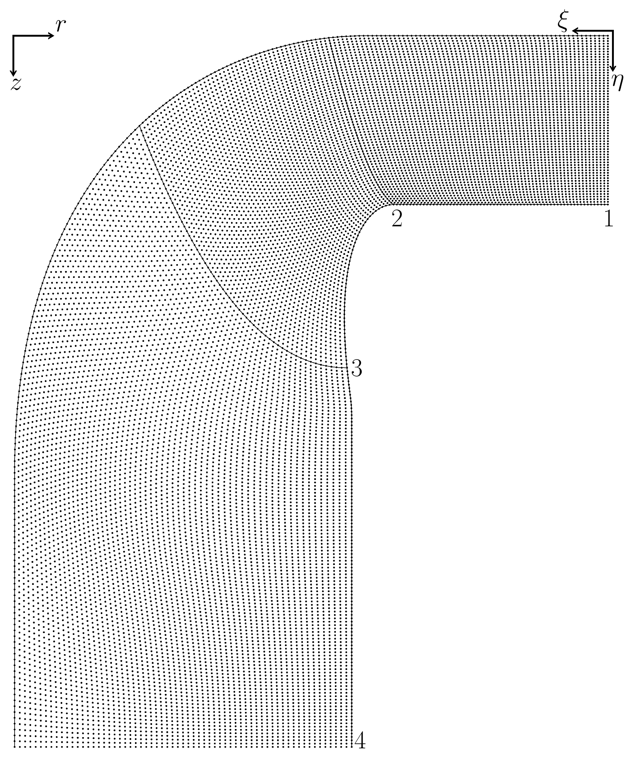
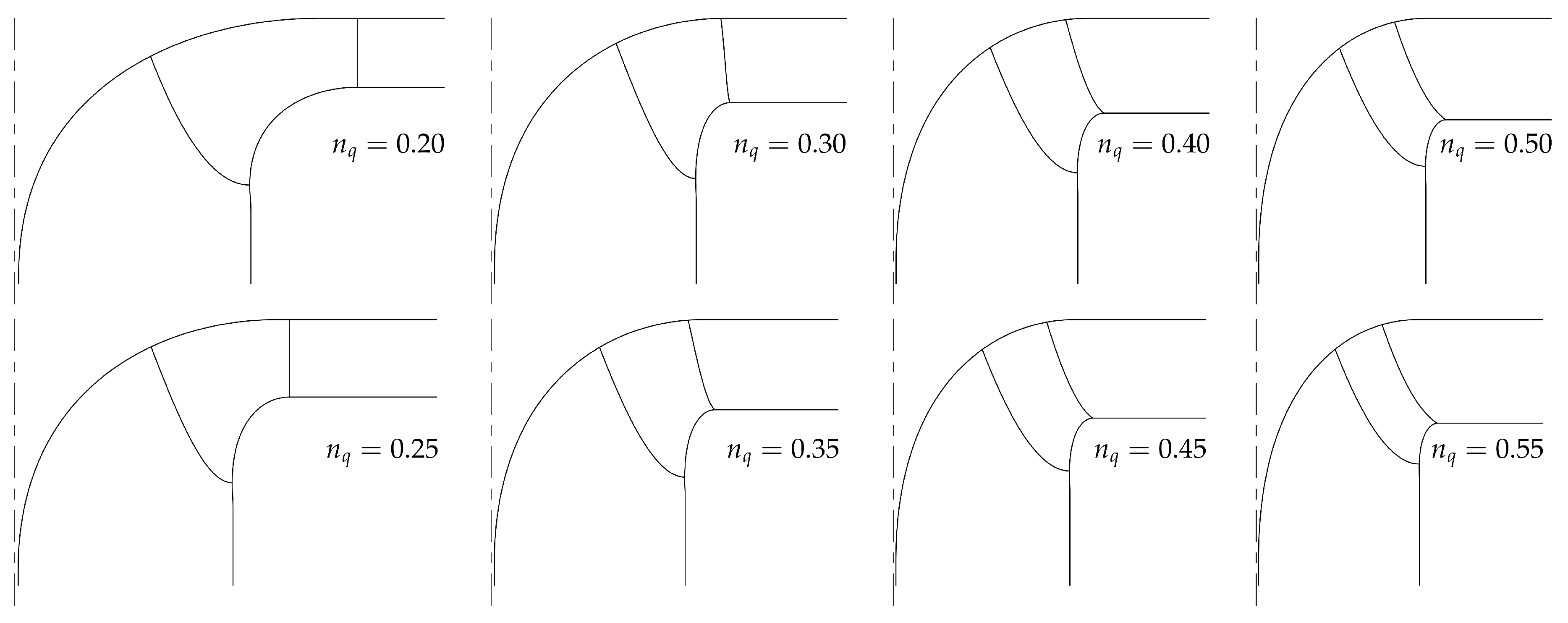
2.4.2. Meridional Channel Geometry Generation

The inverse design method requires the input of the meridional channel geometry, including the hub, shroud, blade leading edge and blade trailing edge meridional projections. The current implementation includes a function that calculates a trail meridional channel geometry that serves as a good starting point; the code can be extended to allow for the input of an arbitrarily parametrized geometry, although this is left for future work.    

Algorithm 1: Implemented inverse design method.

read user inputs

generate meridional channel geometry

generate finite difference mesh

initialize fields and constant integration parameters: f, $t_n$, $r\overline{C}{}_{\theta }$, $\mathsf{\nabla }r\overline{C}{}_{\theta }$, ${\mathsf{\nabla }}^{2}r\overline{C}{}_{\theta }$, $\tilde{\mu }$, $\tilde{\nu }$

while camber surface angle f has not converged do

end

output runner geometry and flow fields

The trail meridional channel geometry is calculated as a function of the available discharge Q, rotational speed $\omega$, and the runner specific speed, defined as

$$n_q=\frac{\omega \sqrt{\frac{Q}{\pi }}}{{\left(2gH\right)}^{\frac{3}{4}}}.$$

(39)

Bovet [15,16] proposed expressions that define the shape of the meridional channel as a function of $n_q$; the shape is then scaled according to a sizing parameter that depends on Q, $\omega$ and $n_q$. The expressions that determine the meridional channel geometry contain 10 parameters that were fitted by Bovet to a database of Francis turbines designed by several manufacturers for a wide variety of operating conditions. In the current implementation, these parameters were updated somewhat by incorporating the more recent Francis turbine and pump-turbine designs that are reported by Henry [17]. Eight meridional channel geometry examples generated using the present approach are presented in Figure 4.

2.4.3. Discretization and Numerical Methods

As illustrated in Figure 3, the meridional channel domain is discretized with a mesh that conforms to the blade leading and trailing edges. Finite difference approximations are used to discretize the differential operators: $\frac{\partial }{\partial \xi }$, $\frac{\partial }{\partial \eta }$, $\frac{{\partial }^2}{\partial {\xi }^2}$ and $\frac{{\partial }^2}{\partial {\eta }^2}$. Second-order accurate central differences are used for interior nodes, whereas second-order one-sided approximations are used for the boundary nodes [18]. Equivalent finite difference approximations are used to calculate the components of the Jacobian $\mathit{J}$, needed to compute the mesh metric coefficients, i.e., $\alpha$, $\beta$, $\gamma$, J, $\tau$, and $\sigma$.

The implicit algorithm used to solve the mean and periodic flow equations entails the solution of a large sparse linear systems assembled from the finite difference approximations of each term present in the respective governing equation. The iterative biconjugate gradient stabilized method (BiCSTAB) is used, together with an incomplete lower-upper (ILU) factorization of the system matrix as a preconditioner.

The blade camber surface equation is solved by integrating along the flow streamlines on the blade surface, which is to say along the characteristic curves of the equation. The camber surface angle f at the blade leading edge, i.e., the stacking condition, is used as initial condition for this integration. As evidenced in Figure 5a, the mean flow streamlines tend to recede from the hub and concentrate towards the shroud. Furthermore, during the initial iterations the periodic flow velocity is of considerable magnitude and may further disrupt the streamlines, making their distribution much less homogeneous. This implies that, when integrating equispaced streamlines starting at the blade leading edge, some blade regions may end up sparsely populated, resulting in significant interpolation error when calculating f at nodes that are relatively far from the closest integrated streamline.

To address this problem, the integration is performed in steps. For each of the nodes in a given grid line defined by constant $\eta$-coordinate, the streamline is integrated backwards using the second-order accurate Crank-Nicolson scheme until the upstream grid line is intersected; the calculated $\delta f$ is used, together with the f value interpolated at the intersection with the upstream grid line, to compute the new f value at the node from which the streamline originated. This process is repeated from leading edge to trailing edge, as illustrated in Figure 5b, ensuring a uniform distribution of streamline sections and therefore avoiding the aforementioned interpolation error.

Once the camber surface angle $f^{\mathrm{new}}$ that respects the current flow field is calculated, a relaxation factor ${\varphi }_f$ is used to compute the updated camber surface angle as $f=f^{\mathrm{new}}{\varphi }_f+f^{\mathrm{old}}(1-{\varphi }_f)$. The relaxation factor ensures stability of the algorithm by damping the variation of the camber surface angle; ${\varphi }_f$ is adaptively selected according to

$${\varphi }_f=min[max(0.60-\frac{{\left|\mathsf{\Delta }f\right|}_{l^2}^{0.6}}{25},0.05),max(0.60-\frac{{\left|\mathsf{\Delta }f\right|}_{l^{\infty }}^{0.4}}{10},0.10\left)\right],$$

(40)

where ${\left|\mathsf{\Delta }f\right|}_{l^2}$ and ${\left|\mathsf{\Delta }f\right|}_{l^{\infty }}$ are respectively the $l^2$-norm and the $l^{\infty }$-norm, with ${\left|x\right|}_{l^n}=\sqrt[n]{{\sum }_i{\left|x_i\right|}^n}$, calculated over all the grid nodes on the blade, of the variation $\mathsf{\Delta }f=f^{\mathrm{new}}-f^{\mathrm{old}}$. This expression simply states that the relaxation factor is inversely proportional to the magnitude of the blade camber surface angle update, measured in terms of its average and maximum values over the blade; the parameters were fine-tuned based on extensive testing over several geometries. The relaxation factor ${\varphi }_f$ is typically close to 0.5.

An additional stability measure that is implemented is to scale the periodic velocity by a factor ${\varphi }_{\mathit{c}}$, which is smoothly relaxed from a value of ${\varphi }_{\mathit{c}}=0.5$ at the first iteration to a value of ${\varphi }_{\mathit{c}}=1$ from the tenth iteration onwards.

The solution convergence is assessed based on ${\left|\mathsf{\Delta }f\right|}_{l^2}$ over the blade grid nodes and $|\frac{\mathsf{\Delta }\mathit{C}}{\mathit{C}}{|}_{l^2}$ over all nodes. In other words, for a solution to be considered converged, the variation of both the blade camber surface angle and the velocity field between successive iterations must fall below an arbitrary threshold value, typically 0.1° and $0.1\%$, respectively.

3. Characterization and Validation of the Inverse Method Implementation

3.1. Convergence Analyses

In this section the convergence characteristics of the implemented method, both in terms of iterations and discretization resolution, are investigated with the objective of verifying the stability of the method and establishing the grid resolution requirements.

The iterative convergence behavior of the inverse design method is illustrated in Figure 6 for a representative Francis turbine case, using a mesh resolution that guarantees negligible discretization error. Figure 6a presents the $l^2$-norm of the variations $\mathsf{\Delta }f$ and $\frac{\mathsf{\Delta }\mathit{C}}{\mathit{C}}$ between successive iterations as a function of the iteration number. The convergence is mostly monotonic, except for a small bump close to the tenth iteration after which the full periodic velocity is considered by having ${\varphi }_{\mathit{c}}=1$. About 25 iterations are required to achieve a converged solution; a faster convergence is possible for this particular case by setting the relaxation factor ${\varphi }_f\approx 1.0$, although the more conservative adaptive approach is preferred in order to ensure convergence for all cases. Figure 6b evidences the monotonic convergence of the camber surface angle f at five points; the results are normalized by the respective angle value at the last iteration, $f_{35}$. As expected, the points closer to the leading edge ($\widehat{m}=0$) change significantly less than the points further down, in relation to their initialization value $f_1$, given that the camber surface angle at the leading edge is fixed by the stacking condition selected.

The convergence of the method with respect to the mesh resolution has been studied in detail. The grid resolution R is defined such that the number of nodes in the spanwise direction is $2^R+1$. For reference, the mesh illustrated in Figure 3 has $R=6$, implying 65 nodes across the span.

A representative Francis turbine case is used for the grid convergence analysis. The pressure difference across the blade $p^{+}-p^{-}\doteq \mathsf{\Delta }p$ as well as the blade angle ${\beta }_b={tan}^{-1}\left(r\frac{\partial f}{\partial m}\right)$ are selected to assess the convergence, given that these variables depend on the mean and periodic flow velocity components, as well as on the camber surface angle f. A total of 25 points uniformly distributed over the blade and four different resolutions $R=(4,5,6,7)$ are considered.

Figure 7a presents the relative error for ${\tau }_{Ri}={(\mathsf{\Delta }p,{\beta }_b)}_{Ri}$ with respect to the corresponding values computed on the finest grid, ${\tau }_{R7}$. The relative error for each of the 25 points analyzed is illustrated by thin lines, whereas the bold lines represent the average relative error, with error bars computed from the standard deviation. A clear convergence of the solution is evidenced, with the relative error monotonically decreasing with the mesh resolution. For the coarsest mesh the average relative error for the pressure difference is about $2\%$, whereas for the blade angle it is less than $1\%$.

Richardson extrapolation is used to compute the average discretization error. Any given solution metric can be described by the general model $\tau =k_1+k_2\mathsf{\Delta }{x}^{k_3}$, where $\mathsf{\Delta }x$ is the discretization size, $k_3$ is the convergence rate, $k_2$ is a constant and $k_1$ is the converged metric [18]; as such, the discretization error is equal to $k_2\mathsf{\Delta }{x}^{k_3}$. This error model has been independently fitted to the 25 points analyzed, each of which includes the resulting $\mathsf{\Delta }p$ and ${\beta }_b$ at four resolutions.

Figure 7b presents the averaged results of the Richardson extrapolation analysis. The average convergence rate computed is $\overline{k_3}=1.79$, whereas the average discretization error for the coarsest resolution is $2\%$. Note that the error presented in Figure 7b is relative to the finest resolution, which is not necessarily converged; on the contrary, the error presented in Figure 7b is with respect to the converged solution with $\mathsf{\Delta }x\to 0$, implying that it truly is the magnitude of the discretization error.

Even though all the operators in the present implementation are discretized with second-order accurate approximations, the effective convergence rate is $\approx 1.8$, below the formal 2.0. This behavior is probably due to the fact that the number of harmonics N that can be resolved is proportional to the mesh resolution: the source terms of the governing equation for the potential function of the periodic flow, Equation (11), are imaginary exponential functions of frequency proportional to $nB$, with $1\le n\le N$, and therefore the highest order harmonic that can be resolved is subject to the Nyquist–Shannon sampling criterion. If higher order harmonics are used, the source terms suffer from aliasing and inject spurious information into the periodic velocity solution. In short, since the number of harmonics considered increases with the mesh resolution, the convergence rate is slightly below 2.0.

The time to solution, averaged over five runs, for each of the four resolution levels is presented in

Table 1. Convergence study of the inverse design method implementation.

Resolution level R	4	5	6	7	[−]
Number of nodes in spanwise direction: $2^R+1$	17	33	65	129	[−]
Representative discretization error	$\simeq 4$	$\simeq 1.5$	$\simeq 0.5$	$\simeq 0$	[%]
Time to solution	0.051	0.154	1.06	13.4	[min]

. The computations are performed on a single i7-4810MQ CPU core running at 3.8 GHz on Ubuntu Linux 16.04 LTS. It is evidenced that the time to solution increases very significantly with R, given that the number of equations being solved increases with the resolution, as explained above. Although these data are representative of the code performance, the time to solution does depend on other factors such as the turbine geometry: low specific speed runners with long blades tend to have more grid nodes for a given resolution level, since R only depends on the number of nodes along the span, and are therefore relatively more expensive to compute.

Based on these results, it can be concluded that a resolution $R=5$ can be used to efficiently explore the design space at a computational cost of about 10 s per simulation, whereas a resolution $R=6$ can be used to compute the definite mesh-independent results in just over one minute. A considerable speed-up is expected if the code is ported to C++ or another high-performance programming language.

3.2. Implementation Validation

The inverse design method implementation is validated on a Francis turbine case characterized by a specific speed $n_q=0.338$ and a hydraulic power of $156.6$ MW. The blade loading and blade thickness distributions specified are similar to the ones presented in Figure 2, whereas the mesh resolution is selected as $R=6$ to ensure converged results; the corresponding meridional channel discretization is illustrated in Figure 3. The number of blades is set to 16, and a quadratic camber surface angle distribution is specified at the leading edge as the stacking condition, with a $\mathsf{\Delta }f$ of 8.2° at the shroud with respect to the hub. This stacking condition corresponds to an average leading edge slant of ${\tan }^{-1}\left(\frac{r_{LE}\mathsf{\Delta }f}{z_{LE}}\right)={20}^{\circ }$, where $r_{LE}$ is the leading edge radius at the shroud and $z_{LE}$ is the leading edge height. A render of the resulting runner is shown in Figure 8, whilst Figure 9 illustrates the distributions of the blade camber surface wrap angle f and the blade angle ${\beta }_b={tan}^{-1}\left(r\frac{\partial f}{\partial m}\right)$.

The runner geometry output by the method is evaluated using the commercial CFD software ANSYS CFX 19.2, where the Navier–Stokes equations coupled with the $k-\omega SST$ turbulence model are solved in steady-state. Only one blade-to-blade channel is simulated. A mesh with 8.54 million elements and an average dimensionless wall distance over the blade of $\overline{y^{+}}=15.1$ is employed. The velocity orientation and magnitude is prescribed at the inlet, and an average static pressure of 0 Pa is imposed at the outlet.

This simulation configuration is commonplace in the field of hydraulic turbomachines, both in academia and in industry, and has been shown to provide numerical results that are in good agreement with experiments [19,20,21,22,23], at least at the best efficiency operating conditions. Using this well-established CFD methodology is adequate to validate the correctness and physical soundness of the solution obtained with the implemented inverse design method, although it is acknowledged that both numerical solutions will have some degree of discrepancy with respect to physical reality.

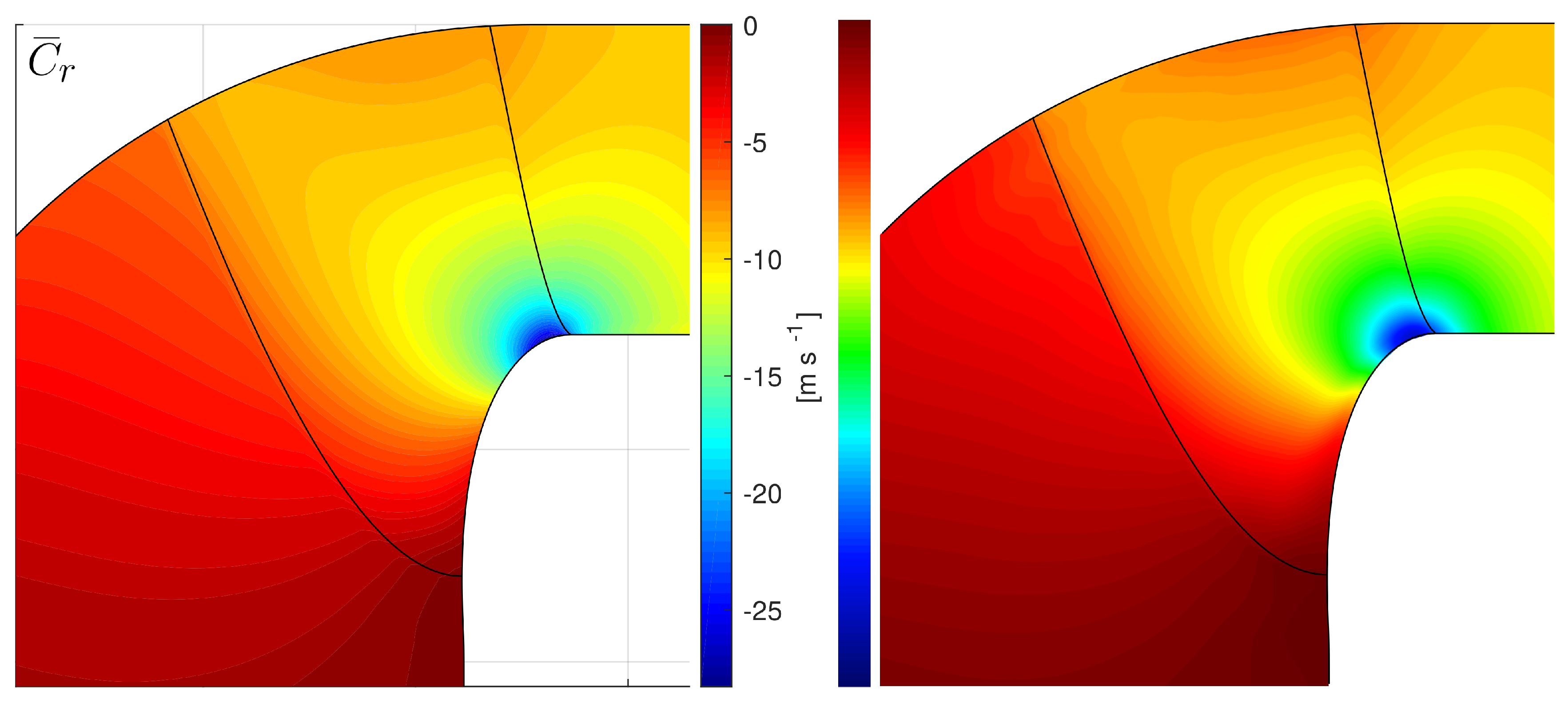
3.2.1. Qualitative Validation

First the velocity fields are used to qualitatively validate the output of the inverse design method implementation. On the following figures, even though the color scale is not identical in matlab and CFX, the same variable range is enforced and both color bars are presented. To further aid in the assessment of the results, the meridional projections of the blade leading and trailing edges, as well as of the hub and shroud, are superimposed on the CFX flow fields. There is a significant agreement for the mean flow velocity magnitude $\overline{C}$, as evidenced in Figure 10. Both the main flow features and the velocity magnitude are well approximated by the present method, compared to the fully-3D Navier–Stokes solution, in spite of the underlying inviscid and axisymmetric mean flow assumptions. The same can be said about the radial and axial mean velocity components, presented in Figure 11 and Figure 12, respectively.

The greatest discrepancy is evidenced in the flow near the shroud, where the mean axial velocity is somewhat overpredicted by the present method. This behavior is most likely a consequence of the inviscid flow assumption. Another divergence occurs for the mean radial velocity prediction near the intersection between the leading edge and the shroud, where the magnitude of the flow acceleration in this high-curvature region is slightly underpredicted by the present method. Overall, a good agreement between both approaches is evidenced.

The comparison of the mean tangential velocity $\overline{C}{}_{\theta }$ is presented in Figure 13. This velocity component illustrates the manner in which the inflow angular momentum is extracted by the runner. As such, the notable agreement achieved validates the proposed methodology by demonstrating that the designed runner accomplishes an essentially complete extraction of the flow angluar momentum. Moreover, not only is the momentum extraction thorough, it is also performed according to the prescribed blade loading distribution, as revealed by the equivalent gradient of $\overline{C}{}_{\theta }$ on both solutions.

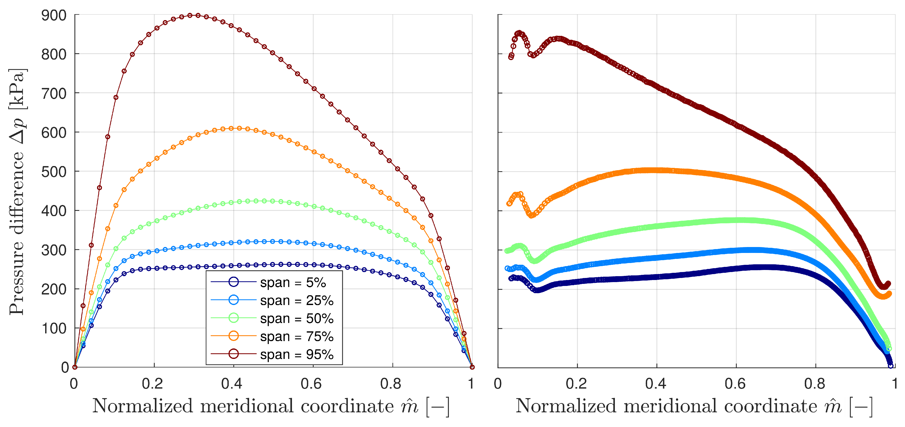
3.2.2. Quantitative Validation

For a quantitative validation of the inverse design method implementation, a comparison of the pressure distribution on the blade along five representative span locations is performed.

The pressure difference $\mathsf{\Delta }p$ across the blade is presented in Figure 14. As revealed by Equation (13), the pressure difference is proportional to $\mathsf{\nabla }r\overline{C}{}_{\theta }$, i.e., proportional to the blade loading, and to the meridional projection of the relative flow velocity, which is greatest towards the shroud. Both of these factors are encompassed in the pressure difference distributions obtained.

There is an overall agreement between the present method results and those calculated with the Navier–Stokes solver, although there are also some noticeable discrepancies that are probably due to a combination of factors, including some error in the computed flow velocity, the assumptions inherent to Equation (13), and the simplifications of the present model. Perhaps the assumption of infinitely thin blades has the greatest impact: it is likely responsible for the underprediction of the pressure difference in the first $8\%$ of the chord, i.e., for $\widehat{m}<0.08$; the method then tends to compensate for this by an overprediction of the pressure difference for $0.20<\widehat{m}<0.40$, especially near the shroud. Based on the five profiles presented in Figure 14, the average relative error of the pressure difference computed with the present method amounts to $12\%$, whereas the relative error in the computed torque is equal to $3\%$. Since the torque is calculated by integration of the pressure difference, a smaller error is expected because, to a certain extent, regions where the pressure difference is underpredicted will cancel out the overcontribution of regions where it is overpredicted. Moreover, at least part of the $3\%$ torque overprediction by the current method is explained by the neglect of all energy losses in the flow.

A comparison of the pressure profiles over the blade is presented in Figure 15. Whereas in the Navier–Stokes solver the pressure is actually computed on each of the blades surfaces, in the current implementation Equation (14) is used to estimate the average meridional pressure $\overline{p}$, and then the computed pressure difference across the blade is symmetrically superimposed: $p_{\mathrm{blade}}^{\pm }=\overline{p}\pm \frac{1}{2}\mathsf{\Delta }p$.

Although there is some agreement in the pressure profiles over the blade between the inverse design method implementation and the Navier–Stokes solution, there are at least two significant discrepancies. The first one has to do with the leading and trailing edges: On the one hand, as already discussed, the assumption of infinitely thin blades hinders the rapid build-up of the pressure at the leading edge, and renders the formation of a stagnation point impossible. On the other hand, there is a pressure jump at the trailing edge near the shroud that is not supposed to be there according to the simplified model. Two possible explanations for that discrepancy are the accumulation of viscous effects or the influence of secondary structures, although no conclusive explanation has been found.

The second significant discrepancy has to do with the repartition of the pressure difference between the suction and pressure sides. It is evident that the simplified approach used to calculate the pressure on each surface, namely a symmetric repartition of the pressure difference, is only approximative. The Navier–Stokes solution suggests that, relative to the mean meridional pressure, the pressure drop on the suction side is greater than the increment on the pressure side.

The energetic efficiency of the runner, computed using the Navier–Stokes solution, is equal to ${\eta }_e=97.8\%$. This value does not consider the energy losses in the guide vanes, which were not modeled, and by definition it does not include the disk friction or leakage discharge losses either. Acknowledging this, the calculated efficiency is considerably high, implying that the implemented inverse design method is actually capable of providing a good hydraulic design that follows the blade loading distribution prescribed as input.

4. Discussion and Outlook

Even though the computational cost of the ANSYS CFX simulation is about 7000 times greater than the present method, the latter is clearly not expected to replace the former: the Navier–Stokes simulations are still necessary to calculate the turbine efficiency, to assess the risk of cavitation, and to study the flow behavior at off-design operating conditions. On the contrary, the two approaches may be complementary: the present inverse design method may be used to quickly identify suitable runner designs that would then be evaluated thoroughly by means of the more expensive and reliable solver.

The blade angle ${\beta }_b$ distribution provided by the inverse design method, presented in Figure 9, is non-monotonic and varies considerably along the span, suggesting that it would not be straightforward to arrive at this geometry by direct parametric manipulation of the blade angles, i.e., by the direct design method. Furthermore, the manner in which these angles affect the flow is unintuitive, whereas the effect of the blade loading on the pressure difference distribution and flow velocity components is more intelligible. It might therefore be advantageous to integrate the present inverse method into the design methodology of Francis runners.

The main assumptions of the model, namely considering the flow as inviscid and the blades as infinitely thin on the periodic flow equations, are expected to introduce only minor error into the design: The blade camber surface angle computed by the method mostly depends on the mean velocity components, which are well predicted as evidenced in Section 3.2.1; this accuracy is partly due to the blockage factor $B_f$, which effectively corrects these velocity components by accounting for the blade thickness. The most important discrepancies were found on the pressure distribution estimated by the method, which has no effect on the output geometry. The pressure distribution is subject to the error introduced by the approximative nature of Equation (14), and by the lack of a stagnation region on the leading edge, itself a consequence of the assumption of infinitely thin blades.

One possible improvement to the method would be to implement a better approximation of the pressure distribution. In the momentum balance used to compute the meridional projection of the pressure gradient, Equation (14), only the axisymmetric mean velocity components were considered, i.e. the gradients in the tangential direction were neglected. Nevertheless, the flow solution does include the complete 3D velocity field by means of the tangential harmonic decomposition, so it is in fact possible to compute all the terms in the momentum balance to derive a better approximation of the pressure gradient. The problem is, however, that the velocity gradients in the tangential direction are subject to the noise introduced by the Gibbs phenomenon near the blade, so a filtering of the spurious oscillations would prove necessary.

Another possible improvement would be to introduce more flexibility and generality into the design method. In the current implementation, it is assumed that the blade leading edge is well aligned with the incoming flow, that the angular momentum at the trailing edge is null, and that the extracted work is constant along the blade span. Although these assumptions are reasonable, they limit the design space and may prevent a widespread use of the method in real applications.

A third development direction lies in the input and output capabilities of the code. It would be beneficial to allow the user to specify an arbitrarily parametrized meridional channel geometry, and to facilitate several output geometry formats compatible with CAD and CFD software, since the current implementation only allows exporting nodal coordinates. Even if these coordinates are sufficient to reconstruct the surfaces and assemble the geometry to be used in the CFD evaluation, this process is unnecessarily cumbersome and could be significantly shortened.

References

1. REN21. Renewables 2018 Global Status Report; Technical Report; Renewable Energy Policy Network for the 21st Century (REN21) Secretariat: Paris, France, 2018. [Google Scholar]
2. Tan, C.S.; Hawthorne, W.R.; McCune, J.E.; Wang, C. Theory of blade design for large deflections: Part II—Annular cascades. ASME J. Eng. Gas Turbines Power 1984, 106, 354–365. [Google Scholar] [CrossRef]
3. Borges, J.E. A three-dimensional inverse design method for turbomachinery: Part I—Theory. J. Turbomach. 1990, 112, 346–354. [Google Scholar] [CrossRef]
4. Borges, J.E. A three-dimensional inverse design method for turbomachinery: Part II—Experimental Verification. J. Turbomach. 1990, 112, 355–361. [Google Scholar] [CrossRef]
5. Zangeneh, M. A compressible three-dimensional design method for radial and mixed flow turbomachinery blades. Int. J. Numer. Methods Fluids 1991, 13, 599–624. [Google Scholar] [CrossRef]
6. Zhu, B.; Wang, X.; Tan, L.; Zhou, D.; Zhao, Y.; Cao, S. Optimization design of a reversible pump-turbine runner with high efficiency and stability. Renew. Energy 2015, 81, 366–376. [Google Scholar] [CrossRef]
7. Zhu, B.; Tan, L.; Wang, X.; Ma, Z. Investigation on flow characteristics of pump-turbine runners with large blade lean. ASME J. Fluids Eng. 2018, 140, 031101. [Google Scholar] [CrossRef]
8. Daneshkah, K.; Zangeneh, M. Parametric design of a Francis turbine runner by means of a three-dimensional inverse design method. IOP Conf. Ser. Earth Environ. Sci. 2010, 12, 012058. [Google Scholar] [CrossRef]
9. Wang, P.; Vera-Morales, M.; Vollmer, M.; Zangeneh, M.; Zhu, B.; Ma, Z. Optimisation of a pump-as-turbine runner using a 3D inverse design methodology. IOP Conf. Ser. Earth Environ. Sci. 2019, 240, 042005. [Google Scholar] [CrossRef]
10. Yang, W.; Liu, B.; Xiao, R. Three-Dimensional Inverse Design Method for Hydraulic Machinery. Energies 2019, 12, 3210. [Google Scholar] [CrossRef] [Green Version]
11. Batchelor, G.K. An Introduction to Fluid Dynamics; Cambridge University Press: Cambridge, UK, 2000. [Google Scholar] [CrossRef]
12. Rishav, R. NURBS Curve. MATLAB Central File Exchange. 2018. Available online: https://www.mathworks.com/matlabcentral/fileexchange/67009-nurbs-curve (accessed on 1 February 2020).
13. Ott, C. Non-Linearly Spaced Vector Generator. MATLAB Central File Exchange. 2017. Available online: https://www.mathworks.com/matlabcentral/fileexchange/64831-non-linearly-spaced-vector-generator (accessed on 1 February 2020).
14. Kumpulainen, P. Tight Subplot. MATLAB Central File Exchange. 2016. Available online: https://www.mathworks.com/matlabcentral/fileexchange/27991-tight_subplot-nh-nw-gap-marg_h-marg_w (accessed on 1 February 2020).
15. Bovet, T. Contribution à l’étude du tracé d’aubage d’une turbine à réaction du type Francis; Technical Report; Informations Techniques Charmilles: Geneva, Switzerland, 1963; Available online: https://infoscience.epfl.ch/record/149853/ (accessed on 1 February 2020).
16. Vivier, L. Turbines hydrauliques et leur régulation: Théorie, construction, utilisation; Albin Michel: Paris, France, 1966. [Google Scholar]
17. Henry, P. Turbomachines hydrauliques: Choix illustré de réalisations marquantes; Presses Polytechniques et Universitaires Romandes: Lausanne, Switzerland, 1992. [Google Scholar]
18. Ferziger, J.; Perić, M. Computational Methods for Fluid Dynamics; Springer: Berlin/Heidelberg, Germany, 1996. [Google Scholar] [CrossRef]
19. Mössinger, P.; Jester-Zürker, R.; Jung, A. Investigation of different simulation approaches on a high-head Francis turbine and comparison with model test data: Francis-99. J. Phys. Conf. Ser. 2015, 579, 012005. [Google Scholar] [CrossRef] [Green Version]
20. Lenarcic, M.; Eichhorn, M.; Schoder, S.J.; Bauer, C. Numerical investigation of a high head Francis turbine under steady operating conditions using foam-extend. J. Phys. Conf. Ser. 2015, 579, 012008. [Google Scholar] [CrossRef]
21. Casartelli, E.; Mangani, L.; Ryan, O.; Del Rio, A. Performance prediction of the high head Francis-99 turbine for steady operation points. J. Phys. Conf. Ser. 2017, 782, 012007. [Google Scholar] [CrossRef] [Green Version]
22. Dewan, Y.; Custer, C.; Ivashchenko, A. Simulation of the Francis-99 hydro turbine during steady and transient operation. J. Phys. Conf. Ser. 2017, 782, 012003. [Google Scholar] [CrossRef] [Green Version]
23. Leguizamón, S.; Ségoufin, C.; Hai-Trieu, P.; Avellan, F. On the efficiency alteration mechanisms due to cavitation in Kaplan turbines. ASME J. Fluids Eng. 2017, 139, 061301. [Google Scholar] [CrossRef]
Figure 1. Blade camber surface example on the cylindrical coordinate system ( r , θ , z ) . The planes defined by θ = [ 0 , π 2 ] illustrate the meridional projection of the blade leading edge (1) and trailing edge (2), as well as the curves that define the axisymmetric shroud (3) and hub (4) surfaces. The blade camber surface is defined by a set of coordinates ( r , θ , z ) , with θ = f ( r , z ) . More generally, the B camber surfaces are defined by θ = i f ( r , z ) , with i = 1 , 2 , , B .
Energies 13 02020 g001
Figure 2. Example distributions of (a) blade loading and (b) normal blade thickness.
Energies 13 02020 g002
Figure 3. Example of a meshed meridional channel domain, composed of: (1) inlet, (2) leading edge, (3) trailing edge, and (4) outlet.
Energies 13 02020 g003
Figure 4. Meridional channel geometry examples for eight values of the specific speed n q .
Energies 13 02020 g004
Figure 5. Mean flow stream function Ψ whose contour lines are the mean flow streamlines (a), and integration along the flow streamlines on the blade surface (b).
Energies 13 02020 g005
Figure 6. Iterative convergence behavior for a typical Francis turbine case. Variation of the camber surface angle and velocity field between successive iterations (a), and convergence of the camber surface angle at midspan at five streamwise positions (b), as functions of the iteration number
Energies 13 02020 g006
Figure 7. Grid convergence behavior for a typical Francis turbine case. Relative error of Δp and βb at 25 points with respect to the finest grid solution (a), and average discretization error computed from Richardson extrapolation of Δp and βb at 25 points (b), as functions of the discretization size Δx.
Energies 13 02020 g007
Figure 8. Render of one quarter of the resulting Francis runner. The pressure and suction surfaces are depicted red and blue, respectively.
Energies 13 02020 g008
Figure 9. Camber surface wrap angle f and blade angle β b , defined as the angle between the blade camber surface tangent and the meridional projection of the streamwise direction.
Energies 13 02020 g009
Figure 10. Mean flow velocity magnitude C ¯ computed using the inverse design method implementation (left) and the ANSYS CFX Navier–Stokes solver (right).
Energies 13 02020 g010
Figure 11. Mean radial velocity C ¯ r computed using the inverse design method implementation (left) and the ANSYS CFX Navier–Stokes solver (right).
Energies 13 02020 g011
Figure 12. Mean axial velocity C ¯ z computed using the inverse design method implementation (left) and the ANSYS CFX Navier–Stokes solver (right).
Energies 13 02020 g012
Figure 13. Mean tangential velocity C ¯ θ computed using the inverse design method implementation (left) and the ANSYS CFX Navier–Stokes solver (right).
Energies 13 02020 g013
Figure 14. Pressure difference across the blade along five span locations computed using the inverse design method implementation (left) and the ANSYS CFX Navier–Stokes solver (right).
Energies 13 02020 g014
Figure 15. Pressure on the blade along five span locations computed using the inverse design method implementation (left) and the ANSYS CFX Navier–Stokes solver (right).
Energies 13 02020 g015