A Coordinated Voltage Control for Overvoltage Mitigation in LV Distribution Grids

Abstract

The design of intelligent strategies for grid management is a cost-effective solution to increase the hosting capacity of distribution grids without investing in the reinforcement of the grid assets. This paper presents a distributed voltage control algorithm to coordinate Energy Storage Systems (ESSs) and Distributed Generation (DG) in a scenario of high renewable penetration. The proposed control algorithm relies on a dual decomposition approach and aims at mitigating possible voltage rise events occurring in the Low Voltage (LV) grid by solving an optimization problem of power minimization. Instead of using local control strategies, in the proposed solution, the voltage control burden is distributed among all the available resources in the grid, which cooperate to resolve the existing voltage violations. The performance of the developed voltage control has been tested under realistic distribution grid scenarios, using stochastic load profiles together with photovoltaic generation profiles obtained in the presence of both clear sky and cloudy sky conditions. The algorithm is also compared to a strategy that considers only DG management, highlighting the benefits associated to the proposed coordination of DG and Energy Storage Systems (ESSs).

1. Introduction

With the ongoing decarbonisation of the energy sector, electric distribution grids will need to accommodate a more and more massive share of Distributed Generation (DG), mainly based on Renewable Energy Sources (RES). The high penetration of DG can pose severe challenges in terms of network management, not only because of the transition from passive to active grids, but also due to the possible occurrences of overvoltage and overloading events. DG integration can be challenging in particular for Low Voltage (LV) grids, where most of the small-scale photovoltaic (PV) systems are installed [1] and where the generation capacity can be even several times larger than the peak load [2,3]. The possible solutions to increase the so-called hosting capacity of the LV grid, while preventing the technical issues associated to overvoltages and overloads, can be classified in two main categories: (i) reinforcing the grid through specific reinforcement measures; (ii) employing smart control tools to ensure the management of the DG during critical conditions [4,5]. Even if investing in the physical assets (e.g., replacing substation transformers or laying additional cables) is often the preferred solution of Distribution System Operators (DSOs), studies prove that adopting smart management solutions is not only more environmentally friendly and less invasive, but also economically convenient [6,7]. Moreover, in Europe, the European Commision recently issued the so-called Clean Energy Package, which recommends measures and incentives to foster software-based solutions [8]. This could play a key role to encourage DSOs to invest more in digitalization and smartness rather than in physical assets.

Focusing on the problem of voltage rise mitigation through smart control, a number of different voltage control solutions has been recently proposed in the scientific literature. The proposed control strategies can be distinguished depending on their communication and architectural requirements. The simplest solutions rely on local control approaches, which depend only on the power generation or on the measurements collected at the point of common coupling of the DG [9,10]. The main benefit of such approaches is their simplicity, since they do not require any information exchange with other resources or components in the grid, thus avoiding the need for a dedicated Information and Communication Technology (ICT) infrastructure. At the same time, however, such solutions usually do not allow an optimal management of the DG resources and could lead to unnecessary curtailments of active power, when local energy management systems are not installed [11]. Moreover, local solutions do not exploit the available distributed components, which could lead to a globally non-optimal solution [12]. For this reason, alternative control strategies based on centralized or decentralized architectures have also been proposed in the literature [13,14,15,16]. Centralized architectures generally permit designing optimal DG management policies, but they also require the communication of all the field data to a control center and subsequently to send the control commands back to the DG in the grid [17]. On the other hand, decentralized approaches can provide sub-optimal results (or converge towards the optimum only after a certain number of iterations), but they have the advantage of requiring only limited communication among the available resources, with no need for a centralized supervisor and instead with the possibility to directly implement the control logic at the DG.

In general, regardless of the control architecture, all the DG management approaches allow for the regulation of the voltage profile by acting on the reactive power injection/absorption and via the control of the generated active power (sometimes also referred to as feed-in management) [1]. As a matter of fact, in presence of excessive generation, all the control solutions eventually lead to a curtailment of the generated active power. In this regard, a possible way to avoid the renewable energy curtailment, while keeping the grid voltage within the allowed boundaries, is to involve other flexible Distributed Energy Resources (DERs) available in the grid in a more complex management schema. In the smart grid scenario, for example, final customers could play an active role by supporting the operation of the grid through a flexible reshaping of their power demand via so-called demand side management scheme [18]. Another option, which is more and more commonly available in combination with PV systems, is the use of Energy Storage Systems (ESSs) [19,20,21]. With the availability of distributed ESSs, the exceeding power generated from the DG can be temporarily stored to avoid any voltage violations and then be re-injected into the system when the operating conditions of the grid are farther from the operational boundaries. Such a strategy clearly requires a coordinated management of DG and ESSs in order to optimize the use of the available DERs.

With reference to this scenario, this paper presents a coordinated control solution for the management of both DG and ESSs in LV distribution grids, in order to solve possible overvoltage issues. The theory behind the control algorithm is derived from Reference [16] and it is here adapted to consider the simultaneous management of reactive power through the DG and of active power through the ESSs. The same control philosophy is then used to manage also the curtailment of DG active power, which can be needed if the other countermeasures are not sufficient to resolve the voltage violations. The algorithm allows weighting the participation of DG and ESSs in the voltage regulation process and to flexibly decide how much each DG and ESS component contributes to the mitigation of overvoltage or undervoltage events. The resulting control can be implemented in a decentralized way, hence requiring only limited communication and information exchange among the different DG and ESSs in the grid. The overall control scheme has been tested using realistic distribution grid scenarios, taking into account the highly dynamic power fluctuations that can be typically found in distribution systems. Overall, the contributions of this paper are thus: (i) combine the control of reactive power in the DG with the management of the active power in the ESSs thus extending the logic presented in Reference [16]; (ii) to propose a decentralized algorithm that can flexibly adjust the participation of different DG and ESSs in the voltage regulation process; (iii) to test and validate the proposed algorithm in realistic conditions that are likely to occur in the distribution system.

The remainder of this paper is structured as follows. Section 2 gives an overview of the technical aspects behind the occurrence of overvoltages due to the DG integration and of the mitigation possibilities through the regulation of the active/reactive power of DG or storage systems. Section 3 presents the details of the coordinated control of DG and ESSs proposed for solving the voltage rise issues. The designed coordinated control has been then validated and assessed via ad hoc tests: Section 4 describes the used simulation set-up, while Section 5 presents and discusses the obtained results. Finally, Section 6 gives the final remarks and concludes the paper.

2. Challenges of DG Integration

The growing penetration of DG is drastically changing the way distribution grids operate. In particular, increasing levels of DG can lead to bi-directional power flows, injection of power into the upper voltage level grid, possible overloading of power system lines/components as well as voltage rises along the feeders. This section briefly summarizes the theoretical aspects behind the occurrence of voltage rise events due to the excessive DG penetration and introduces the possible countermeasures via the active/reactive power control of DG and ESSs.

2.1. Voltage Rise

As previously described, the presence of DG leads to the possibility of reverse power flows and, consequently, to the possible increase of the voltage magnitude along the nodes. This, in scenarios with very large DG penetration, can eventually turn into overvoltage conditions. The effect of the injection of active and reactive power into the grid nodes of a radial distribution network can be described through the following linearized branch-flow model [17,22], which formalizes the dependence of the node voltage from the power flowing in the branches:

$$v_i=v_0+\sum _{(j,k)\in L_i}{z}_{j,k}(\sum _{h\in \beta (k)}(s_h^{g*}-s_h^{c*})).$$

(1)

Equation (1) describes a 3-phase balanced radial distribution feeder where $L_i$ is the set of branches (with sending node j and receiving node k) on the path from bus 0 to bus i; $z_{j,k}$ is the impedance of the generic branch between nodes j and k; $\beta (k)$ is the set of all the descendants of node k; $s_h^{g*}$ represents the complex conjugate of the power ($p_h^g-j{q}_h^g$) injected in the grid at the generation node h; $s_h^{c*}$ is the complex conjugate of the power ($p_h^c-j{q}_h^c$) consumed at the load node h; $v_i$ and $v_0$ are the voltage phasors at node i and at the slack bus, respectively.

The relationship in (1) holds when considering per unit quantities, neglecting the high order real and reactive power loss terms and with the approximation that $v_i\approx 1p.u.$ (with this assumption, the current phasor injections can be replaced with the corresponding complex power injections). Using as an example the 3-bus system depicted in Figure 1 ($i=0,1,2$), the voltage at the buses along the feeder can be thus calculated as follows:

$$\begin{array}{ccc}{v}_1\hfill & =& v_0+z_{01}(s_1^{g*}-s_1^{c*})+z_{01}(s_2^{g*}-s_2^{c*})\hfill \\ v_2\hfill & =& v_0+z_{01}(s_1^{g*}-s_1^{c*})+(z_{01}+z_{12})(s_2^{g*}-s_2^{c*}).\hfill \end{array}$$

(2)

Equation (1) can be rewritten in a more general and compact form as follows:

$$v_i=v_0+\sum _{(j,k)\in \mathsf{\Gamma }}{\mathbf{Z}}_{j,k}(s_k^{g*}-s_k^{c*})),$$

(3)

where $\Gamma$ is the set of grid buses and $\mathbf{Z}$ is a matrix containing the mutual voltage-to-power-injection sensitivity factors given by the sum of branch impedances resulting in (1).

As shown in Reference [16], the matrix $\mathbf{Z}$ can be easily obtained starting from the admittance matrix $\mathbf{Y}$ of the grid, by solving the following equation system:

$$\left[\begin{array}{cc}\mathbf{Z}& \mathbf{1}\\ {\mathbf{1}}^T& 0\end{array}\right]={\left[\begin{array}{cc}\mathbf{Y}& {\mathbf{1}}_0\\ {\mathbf{1}}_0^T& 0\end{array}\right]}^{-1},$$

(4)

where $\mathbf{1}$ is a column vector of ones and ${\mathbf{1}}_0$ is a column vector with value 1 in position 0 and zeros elsewhere. With the definition of the matrix $\mathbf{Z}$, and writing voltages, generated powers and consumed powers at the nodes of the grid as N-size column vectors, where N is the number of nodes, the equation of the bus voltages can be rewritten as:

$$\mathbf{v}=\mathbf{1}{v}_0+\mathbf{Z}({\mathbf{s}}^{g*}-{\mathbf{s}}^{c*}).$$

(5)

The branch-flow formulation in (5) has general validity (it applies also to meshed grids) and it allows understanding how the voltage varies along the nodes depending on the profiles of power consumption and generation. In the following, this equation will be used to understand how DG and ESSs can be controlled to regulate the voltage profile.

2.2. DG Active and Reactive Power Regulation

Expanding the terms in Equation (5) and considering a voltage phase angle equal to zero at the slack bus, the vector of the voltages at the different nodes of the grid can be expressed as:

$${\mathbf{v}}_{re}+j{\mathbf{v}}_{im}=\mathbf{1}{V}_0+(\mathbf{R}+j\mathbf{X})({\mathbf{p}}^g-j{\mathbf{q}}^g-{\mathbf{p}}^c+j{\mathbf{q}}^c),$$

(6)

where ${\mathbf{v}}_{re}$ and ${\mathbf{v}}_{im}$ are the real and imaginary components of the voltage phasor vector, $V_0$ is the voltage magnitude at the slack bus, and R and X are the real and imaginary part of the impedance matrix Z.

Since electrical grids are usually operated with large power factors, generally it is possible to approximate ${\mathbf{v}}_{re}\approx \mathbf{V}$. Using this approximation, from (6), the vector of the resulting bus voltage magnitudes is:

$$\mathbf{V}=\mathbf{1}{V}_0+\mathbf{R}({\mathbf{p}}^g-{\mathbf{p}}^c)+\mathbf{X}({\mathbf{q}}^g-{\mathbf{q}}^c).$$

(7)

Equation (7) shows that a positive unbalance between generation and load (generation larger than the loads) causes an increase of the voltage, while prevailing loads lead to voltage drops along the grid. The level of voltage rises (or drops) is directly associated to the entity of the mismatch between generation and load as well as to the magnitude of the branch impedances (e.g., rural grids with long lines and high impedances are more likely to experience significant deviations with respect to the starting voltage at the slack bus). An overvoltage event occurs when the voltage exceeds the allowed thresholds at one or more nodes of the network. The power quality standard EN 50160 defines an allowed voltage band of $\pm 10\%$ around the nominal voltage of the grid for the rms voltages calculated over 10 minutes [23]. However, stricter requirements can exist in the national grid codes or in the interconnection guidelines of each DSO. In Germany, for example, the VDE AR-N4105 sets a limit of $3\%$ for the maximum voltage rise caused by PV plants in LV grids [24].

From (7), it can be observed that the possible mitigation of overvoltage events via the DG control can be obtained either by curtailing the generated active power ${\mathbf{p}}^g$ or by absorbing reactive power (in this case, the injected reactive power ${\mathbf{q}}^g$ at the generation node would become negative). Indicating with $\Delta {\mathbf{p}}^{DG}$ the curtailment of active power generation and with $\Delta {\mathbf{q}}^{DG}$ the increase of absorbed reactive power at the generation nodes, the DG-controlled voltage can be thus expressed as:

$${\mathbf{V}}^{*}=\mathbf{1}{V}_0+\mathbf{R}({\mathbf{p}}^g-\Delta {\mathbf{p}}^{DG}-{\mathbf{p}}^c)+\mathbf{X}({\mathbf{q}}^g-\Delta {\mathbf{q}}^{DG}-{\mathbf{q}}^c).$$

(8)

Comparing (8) and (7), it is clear that the voltage reduction $\Delta {\mathbf{V}}^{DG}$ determined by the DG control results:

$$\Delta {\mathbf{V}}_{DG}=\mathbf{R}·\Delta {\mathbf{p}}^{DG}+\mathbf{X}·\Delta {\mathbf{q}}^{DG}.$$

(9)

The relationship above is at the basis of many different DG control strategies, which vary only for the particular coordination or prioritization of the active and reactive power control actions. The same relationship will be used also in Section 3 to derive the objective function of the proposed control algorithm.

2.3. Energy Storage System Management

One of the weaknesses of control strategies solely based on the DG regulation is the need to curtail the active power when overvoltages are too large. In fact, if the DG is based on RES, this results into a waste of potentially available clean energy. ESSs can resolve this weakness thanks to the possibility of flexibly storing the surplus of generation. In general, ESSs can be seen as equivalent to consumption units when charging or as equivalent generation units when discharging. In this paper, it is assumed that ESSs are controlled so that they always absorb or inject active power. Using this assumption, Equation (7) can be modified as follows to explicitly take into account the charging/discharging behaviour of the storage:

$$\mathbf{V}=\mathbf{1}{V}_0+\mathbf{R}({\mathbf{p}}^g+{\mathbf{p}}^{ESS,dis}-{\mathbf{p}}^c-{\mathbf{p}}^{ESS,ch})+\mathbf{X}({\mathbf{q}}^g-{\mathbf{q}}^c),$$

(10)

where ${\mathbf{p}}^{ESS,dis}$ and ${\mathbf{p}}^{ESS,ch}$ are the discharging and charging active powers of the ESSs, respectively.

From (10), it is immediate to see that reducing the discharging and/or increasing the charging of the ESSs leads to voltage reductions, thus achieving the objective of voltage rise mitigation. At the same time, the stored power can be re-injected in the grid at a later time, when the loads exceed the available generation, in order to fulfil the load demand and attenuate the voltage drops in the grid. In this way, the ESSs allow both supporting the grid operation and fully exploiting the available energy coming from RESs. Indicating with $\Delta {\mathbf{p}}_{ESS}$ the increase of power from the grid to the storage (which can correspond to both a decrease of discharing power or an increase of charging power), the new voltage determined by the ESS control can be written as:

$$\mathbf{V}=\mathbf{1}{V}_0+\mathbf{R}({\mathbf{p}}^g+{\mathbf{p}}^{ESS,dis}-{\mathbf{p}}^c-{\mathbf{p}}^{ESS,ch}-\Delta {\mathbf{p}}^{ESS})+\mathbf{X}({\mathbf{q}}^g-{\mathbf{q}}^c)$$

(11)

from which the voltage reduction effect $\Delta {\mathbf{V}}_{ESS}$ (comparing (11) to (10)) can be found to be:

$$\Delta {\mathbf{V}}_{ESS}=\mathbf{R}·\Delta {\mathbf{p}}^{ESS}.$$

(12)

In the following of this paper, ESSs are considered to be always available when needed to contribute for voltage control. To be considered available, the ESSs should have a value of SOC that guarantees the absorption or injection of active power to compensate for the overvoltage or undervoltage respectively. Possible uses of the ESSs for additional purposes (e.g., other ancillary services, consumers self-consumption optimization, etc.) are not taken into account, implicitly assuming that they do not affect the availability of the ESSs when they are called to participate in the voltage control. This assumption, which is mostly theoretical, is used in this paper to allow the proof of concept validation of the proposed control scheme and to demonstrate the impact of the ESSs on the voltage regulation process. When considering the contribution of the ESSs, the resulting voltage reduction (13) is the sum of (9) and (12).

$$\Delta \mathbf{V}=\Delta {\mathbf{V}}_{ESS}+\Delta {\mathbf{V}}_{DG}.$$

(13)

3. Coordinated Voltage Control

The objective of the proposed control algorithm is to minimize the contributions of active and reactive power injection, coming from the DG and ESSs, that are needed to keep the voltage within the allowed limits. To this purpose, the active and reactive power contributions are weighted with $\mathbf{R}$ and $\mathbf{X}$, respectively, according to the impact (shown in Equations (9) and (12)) that they bring on the voltage magnitude reduction. At the same time, the contribution of the active and reactive powers is expressed in squared terms, so that a quadratic formulation can be obtained. Overall, the voltage control logic is thus expressed as a minimization problem having the following objective function, where the terms related to active power curtailment and active power injections of the ESSs are added to the function defined in Reference [11]:

$$J={\Delta {\mathbf{p}}^{ESS}}^T\mathbf{R}\Delta {\mathbf{p}}^{ESS}+{\Delta {\mathbf{p}}^{DG}}^T\mathbf{R}\Delta {\mathbf{p}}^{DG}+{\Delta {\mathbf{q}}^{DG}}^T\mathbf{X}\Delta {\mathbf{q}}^{DG}.$$

(14)

Looking at the particular structure of the vectors $\Delta {\mathbf{p}}^{ESS}$, $\Delta {\mathbf{p}}^{DG}$ and $\Delta {\mathbf{q}}^{DG}$ (these are N-size vectors whose elements will be equal to zero for all the nodes where there is no ESS or DG, respectively), it is possible to find that (14) can be further modified in the following form:

$$J={\Delta {\mathbf{p}}_{+}^{ESS}}^T{\mathbf{R}}^{ESS}\Delta {\mathbf{p}}_{+}^{ESS}+{\Delta {\mathbf{p}}_{+}^{DG}}^T{\mathbf{R}}^{DG}\Delta {\mathbf{p}}_{+}^{DG}+{\Delta {\mathbf{q}}_{+}^{DG}}^T{\mathbf{X}}^{DG}\Delta {\mathbf{q}}_{+}^{DG},$$

(15)

where:

• ${\mathbf{R}}^{ESS}=Re{\left\{{\mathbf{Z}}_h\right\}}_{h\in ESS}$ is the real part of the submatrix ${\mathbf{Z}}_h$ obtained when considering only the rows and columns of Z associated to the nodes h where the ESSs are connected.
• ${\mathbf{R}}^{DG}=Re{\left\{{\mathbf{Z}}_h\right\}}_{h\in DG}$ is the real part of the submatrix ${\mathbf{Z}}_h$ obtained when considering only the rows and columns of Z associated to the nodes h where DGs are connected.
• ${\mathbf{X}}^{DG}=Im{\left\{{\mathbf{Z}}_h\right\}}_{h\in DG}$ is the imaginary part of the submatrix ${\mathbf{Z}}_h$ obtained when considering only the rows and columns of Z associated to the nodes h where DGs are connected.
• $\Delta {\mathbf{p}}_{+}^{ESS}$, $\Delta {\mathbf{p}}_{+}^{DG}$ and $\Delta {\mathbf{q}}_{+}^{DG}$ are the subvectors of $\Delta {\mathbf{p}}^{ESS}$, $\Delta {\mathbf{p}}^{DG}$ and $\Delta {\mathbf{q}}^{DG}$ associated to the only nodes where ESSs and DG are present, respectively.

From (15), the optimization problem as a function of $\Delta {\mathbf{p}}_{+}^{ESS}$, $\Delta {\mathbf{p}}_{+}^{DG}$ and $\Delta {\mathbf{q}}_{+}^{DG}$ is expressed as:

$$\begin{array}{cccc}\hfill & \underset{p,q}{\mathrm{minimize}}\hfill & \hfill & {\Delta {\mathbf{p}}_{+}^{ESS}}^T{\mathbf{R}}^{ESS}\Delta {\mathbf{p}}_{+}^{ESS}+\Delta {{\mathbf{p}}_{+}^{DG}}^T{\mathbf{R}}^{DG}\Delta {\mathbf{p}}_{+}^{DG}+\Delta {{\mathbf{q}}_{+}^{DG}}^T{\mathbf{X}}^{DG}\Delta {\mathbf{q}}_{+}^{DG}\hfill \\ \hfill & \mathrm{subject}\mathrm{to}\hfill & \hfill & V_{min}\le \mathbf{V}\le V_{max},\hfill \\ \hfill & \hfill & \hfill & \Delta {\mathbf{p}}_{min}^{ESS}\le \Delta {\mathbf{p}}^{ESS}\le \Delta {\mathbf{p}}_{max}^{ESS},\hfill \\ \hfill & \hfill & \hfill & \Delta {\mathbf{p}}_{min}^{DG}\le \Delta {\mathbf{p}}^{DG}\le \Delta {\mathbf{p}}_{max}^{DG},\hfill \\ \hfill & \hfill & \hfill & \Delta {\mathbf{q}}_{min}^{DG}\le \Delta {\mathbf{q}}^{DG}\le \Delta {\mathbf{q}}_{max}^{DG}\hfill \end{array}$$

(16)

Given that the ESSs and the DG do not have any explicit interaction, the solution of the minimization problem can be decoupled into three separate problems, thus resulting into:

$\Delta V(\Delta p_{ESS})$ minimization

$$\begin{array}{cccc}\hfill & \underset{p^{ESS}}{\mathrm{minimize}}\hfill & \hfill & \Delta {\mathbf{p}}_{+}^{{ESS}^T}·{\mathbf{R}}^{ESS}·\Delta {\mathbf{p}}_{+}^{ESS}\hfill \\ \hfill & \mathrm{subject}\mathrm{to}\hfill & \hfill & V_{min}\le V_h\le V_{max},\hfill \\ \hfill & \hfill & \hfill & \Delta p_{h_{min}}^{ESS}\le \Delta p_h^{ESS}\le \Delta p_{h_{max}}^{ESS}\hfill \end{array}$$

(17)

$\Delta V(\Delta p^{DG})$ minimization

$$\begin{array}{cccc}\hfill & \underset{p_{DG}}{\mathrm{minimize}}\hfill & \hfill & \Delta {\mathbf{p}}_{+}^{{DG}^T}·{\mathbf{R}}^{DG}·\Delta {\mathbf{p}}_{+}^{DG}\hfill \\ \hfill & \mathrm{subject}\mathrm{to}\hfill & \hfill & V_{min}\le V_h\le V_{max},\hfill \\ \hfill & \hfill & \hfill & \Delta p_{h_{min}}^{DG}\le \Delta p_h^{DG}\le \Delta p_{h_{max}}^{DG},\hfill \end{array}$$

(18)

$\Delta V(\Delta q_{DG})$ minimization

$$\begin{array}{cccc}\hfill & \underset{q^{PV}}{\mathrm{minimize}}\hfill & \hfill & \Delta {\mathbf{q}}_{+}^{{DG}^T}·{\mathbf{X}}^{DG}·\Delta {\mathbf{q}}_{+}^{DG}\hfill \\ \hfill & \mathrm{subject}\mathrm{to}\hfill & \hfill & V_{min}\le V_h\le V_{max},\hfill \\ \hfill & \hfill & \hfill & \Delta q_{h_{min}}^{DG}\le \Delta q_h^{DG}\le \Delta q_{h_{max}}^{DG},\hfill \end{array},$$

(19)

where $V_h$ represents the voltage at node $h\in ESS$ or $h\in DG$.

In the proposed formulation, the full optimization problem in (16) is split into three smaller sub-problems given by (17)–(19). In each one of the sub-problems, only the active or the reactive power appears; moreover, each sub-problem only concerns a particular type of resource (ESS or DG) and this allows reducing the complexity of the overall minimization process. At the same time, since all the three sub-problems share the same constraint on the allowed voltage boundaries, the obtained control actions indirectly cooperate to resolve the possible voltage rise issues.

Compared to other formulations based on dual decomposition methods [11,17,25], the proposed solution includes the regulation of both the active and reactive power in the grid for the optimization of the voltage profile. This is done taking into account that, in the distribution system, both the active and reactive power at the nodes have an impact on the resulting grid voltage, due to the similar order of magnitude of resistances and reactances of the lines.

3.1. Energy Storage Active Power Control

The process to obtain the feedback control output for the ESSs is based on the well-known duality theory [26] and takes inspiration from the optimization method presented in Reference [16] for the control of the DG reactive power.

The Lagrangian of the problem (17) can be written as:

$$\begin{array}{cc}\hfill & \mathcal{L}(\Delta {\mathbf{p}}_{+}^{ESS},{\mathbf{\lambda }}_{min}^p,{\mathbf{\lambda }}_{max}^p,{\mathbf{\chi }}_{min},{\mathbf{\chi }}_{max})=\Delta {\mathbf{p}}_{+}^{{ESS}^T}·{\mathbf{R}}^{ESS}·\Delta {\mathbf{p}}_{+}^{ESS}+\sum _{h\in N_{ESS}}{\lambda }_{min,h}^p(V_{min}-V_h)+\hfill \\ \hfill & \sum _{h\in N_{ESS}}{\lambda }_{max,h}^p(V_h-V_{max})+\sum _{h\in N_{ESS}}{\chi }_{min,h}(\Delta p_{h_{min}}^{ESS}-\Delta p_h^{ESS})+\sum _{h\in N_{ESS}}{\chi }_{max,h}(\Delta p_h^{ESS}-\Delta p_{h_{max}}^{ESS})\hfill \end{array},$$

(20)

where ${\mathbf{\lambda }}_{min}^p,{\mathbf{\lambda }}_{max}^p,{\mathbf{\chi }}_{min},{\mathbf{\chi }}_{max}$ are the vectors of Lagrangian multipliers associated to the voltage and power constraints, respectively, and $N_{ESS}$ is the set of nodes where an ESS is available.

From the theory of duality, the algorithm is based on the iterative execution of the following steps:

(1)

dual-ascent steps on the dual variables ${\mathbf{\lambda }}_{min}^p,{\mathbf{\lambda }}_{max}^p$;

(2)

dual-ascent steps on the dual variables ${\mathbf{\chi }}_{min},{\mathbf{\chi }}_{max}$;

(3)

unconstrained minimization on the primal variable $\Delta {\mathbf{p}}_{+}^{ESS}$.

Defining with k the iteration of the algorithm, the dual ascent-step 1) is defined as:

$$\begin{array}{cc}\hfill & {\lambda }_{max,h}^p(k+1)={[{\lambda }_{max,h}^p(k)+{\alpha }_{P,ESS}(V_h(k)-V_{max})]}_0^{\infty }\hfill \\ \hfill & {\lambda }_{min,h}^p(k+1)={[{\lambda }_{min,h}^p(k)+{\alpha }_{P,ESS}(V_{min}-V_h(k))]}_0^{\infty }\hfill \end{array},$$

(21)

where ${\alpha }_{P,ESS}$ is a positive constant and the notation ${\left[·\right]}_0^{\infty }$ indicates the projection on the positive orthant.

The calculation of ${\alpha }_{P,ESS}$ is based on Proof of preposition 3 and 4 of Reference [27], resulting in:

$$\begin{array}{c}\hfill {\alpha }_{P,ESS}<\frac{1}{\rho (\mathsf{\Phi }{\mathbf{G}}^{ESS}{\mathsf{\Phi }}^T)},\end{array}$$

(22)

where $\rho$ is the spectral radius, ${\mathbf{G}}^{ESS}$ is defined as ${({\mathbf{R}}^{ESS})}^{-1}$ and $\mathsf{\Phi }={[-{\mathbf{R}}^{ESS},{\mathbf{R}}^{ESS}]}^T$.

For each iteration k, the steps 2) and 3) of the algorithm are calculated with a number of internal iterations K that allows the convergence of 2) and 3) towards the solution of the optimization problem [11].

$$\begin{array}{cc}\hfill & {\chi }_{max,h}(k,K+1)=[{\chi }_{max,h}(k,K)+{\gamma }_{P,ESS}(\Delta p_h^{ESS}(k,K)-\Delta p_{h_{max}}^{ESS})){]}_0^{\infty }\hfill \\ \hfill & {\chi }_{min,h}(k,K+1)={[{\chi }_{min,h}(k,K)+{\gamma }_{P,ESS}(\Delta p_{h_{min}}^{ESS}-\Delta p_h^{ESS}(k,K))]}_0^{\infty }\hfill \end{array},$$

(23)

where ${\gamma }_{P,ESS}$ is a positive constant.

Following the findings in Reference [11], the upper bound for ${\gamma }_{P,ESS}$ to reach a feasible solution is defined as:

$${\gamma }_P<\frac{1}{\rho ({\mathbf{G}}^{ESS})}$$

(24)

where $\rho$ is the spectral radius. To comply with (24), in the implemented algorithm, the value of ${\gamma }_{P,ESS}$ has been chosen to be ${\gamma }_{P,ESS}=\frac{1}{2\parallel {\mathbf{G}}^{ESS}\parallel }$.

The minimization of step 3) with respect to the primal variable is defined as:

$${argmin}_{p^{ESS}}\mathcal{L}(\Delta {\mathbf{p}}_{+}^{ESS},{\mathbf{\lambda }}^p,\mathbf{\chi }).$$

(25)

Since the Lagrangian multipliers are updated via the previously described dual-ascent procedure, in (25), only $\Delta {\mathbf{p}}_{+}^{ESS}$ is considered as an active variable; the unconstrained minimization can be thus expressed as $\frac{\partial \mathcal{L}}{\partial \Delta p_{+}^{ESS}}=0$, which results in:

$$(R^{ESS})·\Delta {\mathbf{p}}_{+}^{ESS}+\frac{\partial \mathbf{V}}{\partial \Delta {\mathbf{p}}_{+}^{ESS}}({\mathbf{\lambda }}_{max}^p-{\mathbf{\lambda }}_{min}^p)+\frac{\partial \Delta {\mathbf{p}}_{+}^{ESS}}{\partial \Delta {\mathbf{p}}_{+}^{ESS}}({\mathbf{\chi }}_{max}-{\mathbf{\chi }}_{min})=0.$$

(26)

From (10), it is possible to find that $\frac{\partial \mathbf{V}}{\partial {\mathbf{p}}_{+}^{ESS}}={\mathbf{R}}^{ESS}$. Therefore, from (26), the updated active power charging for the ESSs (at the iteration k,K+1) becomes:

$$\Delta {\mathbf{p}}_{+}^{ESS}(k,K+1)=-({\mathbf{\lambda }}_{max}^p(k,K+1)-{\mathbf{\lambda }}_{min}^p(k,K+1))-{\mathbf{G}}^{ESS}({\mathbf{\chi }}_{max}(k,K+1)-{\mathbf{\chi }}_{min}(k,K+1)).$$

(27)

Through this process, eventually, the active power associated to the charging of the ESS is projected into its feasible set. By applying the dual ascent method, the optimization problem defined in (17) has thus turned into an algebraic iterative algorithm that can be easily implemented in any programmable language.

As described in Reference [27], it is worth noting that the updates of the Lagrangian multipliers and the calculation of the control output can be performed in a distributed way, given that the resulting ${\mathbf{G}}^{ESS}$ matrix has a particular sparse structure that, for each considered node h, brings dependencies only from its neighbouring ESS nodes. The formulation, however, also highlights a possible drawback associated to the multiplication ${\mathbf{G}}^{ESS}({\mathbf{\chi }}_{max}(k,K+1)-{\mathbf{\chi }}_{min}(k,K+1))$, since the updated values of the multipliers should be exchanged at each iteration K with the neighbors. This can represent a significant burden for the communication, especially when the number K is high. To overcome this problem, the algorithm has been modified to get updated multipliers from the neighbours only at each iteration k, keeping them constant throughout the internal iterations of steps (2) and (3). In this way, the number of times that the multipliers are exchanged can be considerably reduced.

3.2. DG Active Power Control

The control for the curtailment of the active power generated by the DG follows exactly the same procedure described in Section 3.1, but obviously it is applied to the minimization problem (18). As a consequence, the calculation of ${\mathbf{G}}^{DG}$ and ${\gamma }_P$ are based in this case on the matrix ${\mathbf{R}}^{DG}$, while the Lagrangian multipliers are defined as in Section 3.1 but they refer to a different subset ($h\in N_{DG}$) of nodes of the grid. Finally, the positive constants for the dual-ascent algorithm are ${\gamma }_{P,DG}$ and ${\alpha }_{P,DG}$.

3.3. DG Reactive Power Control

The calculation of the reactive power feedback control for the DG follows the same approach as in Section 3.1 and to what was presented in Reference [11], which can be summarized as follows. The Lagrangian of the problem (19) can be written as:

$$\begin{array}{cc}\hfill & \mathcal{L}(\Delta {\mathbf{q}}_{+}^{DG},{\mathbf{\lambda }}_{min}^q,{\mathbf{\lambda }}_{max}^q,{\mathbf{\mu }}_{min},{\mathbf{\mu }}_{max})=\Delta {\mathbf{q}}_{+}^{{DG}^T}·{\mathbf{X}}^{DG}·\Delta {\mathbf{q}}_{+}^{DG}+\sum _{h\in N_{DG}}{\lambda }_{min,h}^q(V_{min}-V_h)+\hfill \\ \hfill & \sum _{h\in N_{DG}}{\lambda }_{max,h}^q(V_h-V_{max})+\sum _{h\in N_{DG}}{\mu }_{min,h}(\Delta q_{h_{min}}^{DG}-\Delta q_h^{DG})+\sum _{h\in N_{DG}}{\mu }_{max,h}(\Delta q_h^{DG}-\Delta q_{h_{max}}^{DG}),\hfill \end{array}$$

(28)

where ${\mathbf{\lambda }}_{min}^q,{\mathbf{\lambda }}_{max}^q,{\mathbf{\mu }}_{min},{\mathbf{\mu }}_{max}$ are the vectors of Lagrangian multipliers associated to the voltage and power constraints, respectively, and $N_{DG}$ is the set of nodes with a connected generation source.

Similarly to what was presented in Section 3.1, the optimization relies on the iterative execution of two dual-ascent steps and an unconstrained minimization of the primal variable. The first dual-ascent step involves the update of the Lagrangian multipliers associated to the voltage constraints, according to the following:

$$\begin{array}{cc}\hfill & {\lambda }_{max,h}(k+1)={[{\lambda }_{max,h}(k)+{\alpha }_Q(V_h(k)-V_{max})]}_0^{\infty }\hfill \\ \hfill & {\lambda }_{min,h}(k+1)={[{\lambda }_{min,h}(k)+{\alpha }_Q(V_{min}-V_h(k))]}_0^{\infty }\hfill \end{array},$$

(29)

where ${\alpha }_Q$ is a positive constant that has to comply with:

$$\begin{array}{c}\hfill {\alpha }_Q<\frac{1}{\rho (\mathsf{\Phi }{\mathbf{B}}^{DG}{\mathsf{\Phi }}^T)}\end{array},$$

(30)

where $\rho$ is the spectral radius, ${\mathbf{B}}^{DG}$ is defined as ${{\mathbf{X}}^{DG}}^{-1}$ and $\mathsf{\Phi }={[-{\mathbf{X}}^{DG},{\mathbf{X}}^{DG}]}^T$.

The update of the Lagrangian multipliers ${\mu }_{min,h}$ and ${\mu }_{max,h}$ during the second dual ascent step is performed with internal iterations K as described in Section 3.1:

$$\begin{array}{cc}\hfill & {\mu }_{max,h}(k,K+1)={[{\mu }_{max,h}(k,K)+{\gamma }_Q(\Delta q_h^{DG}(k,K)-\Delta q_{h_{max}}^{DG})]}_0^{\infty }\hfill \\ \hfill & {\mu }_{min,h}(k,K+1)={[{\mu }_{min,h}(k,K)+{\gamma }_Q(\Delta q_{h_{min}}^{DG}-\Delta q_h^{DG}(k,K))]}_0^{\infty }\hfill \end{array},$$

(31)

where ${\gamma }_Q$ is a positive constant. Based on the considerations in Reference [11], the upper bound for ${\gamma }_Q$ to reach a feasible solution is defined as:

$${\gamma }_Q<\frac{1}{\rho ({\mathbf{B}}^{DG})},$$

(32)

where $\rho$ is the spectral radius. To comply with (32), the value of ${\gamma }_Q$ has been thus chosen to be ${\gamma }_Q=\frac{1}{2\parallel {\mathbf{B}}^{DG}\parallel }$.

By applying the same approach as in Section 3.1 for the unconstrained minimization of the primal variable, the updated reactive power injections $\Delta {\mathbf{q}}^{DG}$ of the DG (at the iteration k+1) result as:

$$\Delta {\mathbf{q}}_{+}^{DG}(k,K+1)=-({\mathbf{\lambda }}_{max}^q(k,K+1)-{\mathbf{\lambda }}_{min}^q(k,K+1))-{\mathbf{B}}^{DG}({\mathbf{\mu }}_{max}(k,K+1)-{\mathbf{\mu }}_{min}(k,K+1)).$$

(33)

Equation (33) gives a simple algebraic relationship through which it is possible to calculate the updated values of reactive power absorption to be considered for the DG. Similarly to what has been described in Section 3.1, the matrix ${\mathbf{B}}^{DG}$ has a particular sparse structure that, for each node h, brings dependencies only from the neighbouring DG nodes, thus allowing for a distributed implementation of the algorithm. Moreover, to reduce the communication burden of the algorithm, the Lagrangian multipliers can be communicated only at the k-th iteration, thus keeping the same values for the multipliers of the neighbouring nodes during the internal K iterations of the second and third step of the procedure.

3.4. DG and ESS Coordination

As seen in the previous subsections, one of the strengths of the described control algorithm is that the sparse structure of the matrices appearing in the minimization of the primal variable (for all the three sub-problems) leads to dependencies, for each node h, only from the neighbouring nodes, thus allowing for a distributed implementation of the control logic. The described control also allows a simple insertion or removal of actors participating in the control (by acting on the matrices $G_{ESS}$, $G_{DG}$ or $B_{DG}$) and, being a feedback control based on simple algebraic relationships, it requires minimal computational effort [11].

In the proposed approach, a key role for the coordination of the actions performed by the DG and the ESSs is played by the parameters $\alpha$ used for the first step of the dual ascent. The parameters ${\alpha }_{P,ESS}$ and ${\alpha }_Q$ are defined as vectors where each element, which is is associated to an ESS or DG in the grid, can be dynamically modified. Based on the values of these parameters, the role played by each resource in supporting the voltage rise mitigation can be flexibly changed. The variation of ${\alpha }_{P,ESS}$ and ${\alpha }_Q$ modifies the influence that $v_h(k)$ has on the update of the Lagrangian multipliers. In fact, assigning different values of ${\alpha }_Q\left[h\right]$ to the generic node h results in a different update of the Lagrangian multipliers ${\lambda }_{max,h}(k+1)$ and ${\lambda }_{min,h}(k+1)$, which in turn modifies the impact of the overvoltage on the calculation of the active/reactive power set-points.

This feature can be used to prioritize the ESSs charging over the DG reactive power injection in case of overvoltage conditions, or vice versa. For example, the elements of the vector ${\alpha }_Q$ corresponding to the DG nodes can be set to ${\alpha }_Q\left[h\right]\simeq 0$ as long as the multiplier of the associated battery $\chi \left[h\right]$ is equal to zero, meaning that the maximum value of the charging power has not been reached by the ESS yet. With the above logic, the reactive power support is activated only when the ESS charging is not sufficient to limit the overvoltage. The same approach can be applied to the DG active power control described in Section 3.2. In this case, the elements of the vector ${\alpha }_P$ can be kept equal to zero till when the reactive power absorption or the charging power of that node and of the neighbours have not reached the maximum, meaning that the associated multipliers are still equal to zero.

An additional logic can be used to remove one or more ESSs from the list of resources available for the control of the grid by defining ${\alpha }_{P,ESS}\left[h\right]=0$. Such a logic can be useful, for example, when a battery is fully charged (or it is charged beyond a certain threshold value) and it is preferable not to exploit it any longer for the voltage mitigation purposes.

3.5. Addition of Virtual Nodes

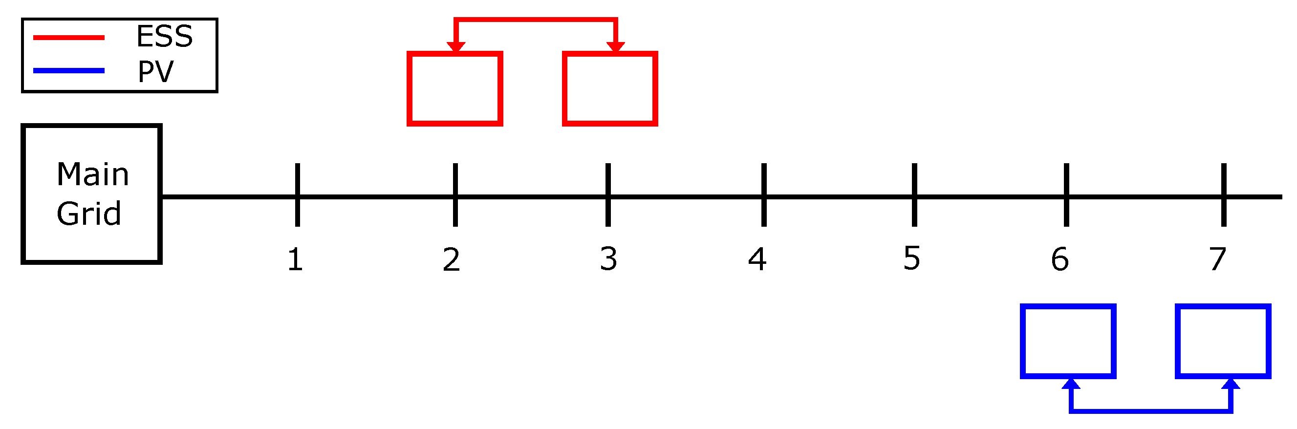
As described in Section 3.1 and Section 3.3, the distributed control algorithm is based on the communication of Lagrangian multipliers between the neighbouring ESS or DG nodes, which comes from the sparsity of the matrices ${\mathbf{G}}^{ESS}$ and ${\mathbf{B}}^{DG}$ (or ${\mathbf{G}}^{DG}$), respectively. Moreover, the control of ESSs and DG is decoupled, which allows reducing the complexity of the control strategy. While this has clear benefits from a computational burden perspective, it can also lead to an ineffective control in specific scenarios. In particular, this can happen when the controllable resources are located only in nodes where the overvoltages do not appear (typically at the beginning of the feeder), thus leading to a situation where no issue is detected and consequently the resources are not activated to contribute to the overvoltage mitigation. This type of scenario is described through a simple example in Figure 2. In the example, ESSs are assumed to be installed only at nodes 2 and 3, while DG is present at buses 6 and 7. According to the logic described in the previous subsections, both ESSs and DG act independently and communicate only with the neighbouring nodes equipped with the same type of resource. As a result, with this configuration, if an overvoltage occurs at the end of the feeder, the ESSs will not be able to detect the problem and to react for resolving the overvoltage.

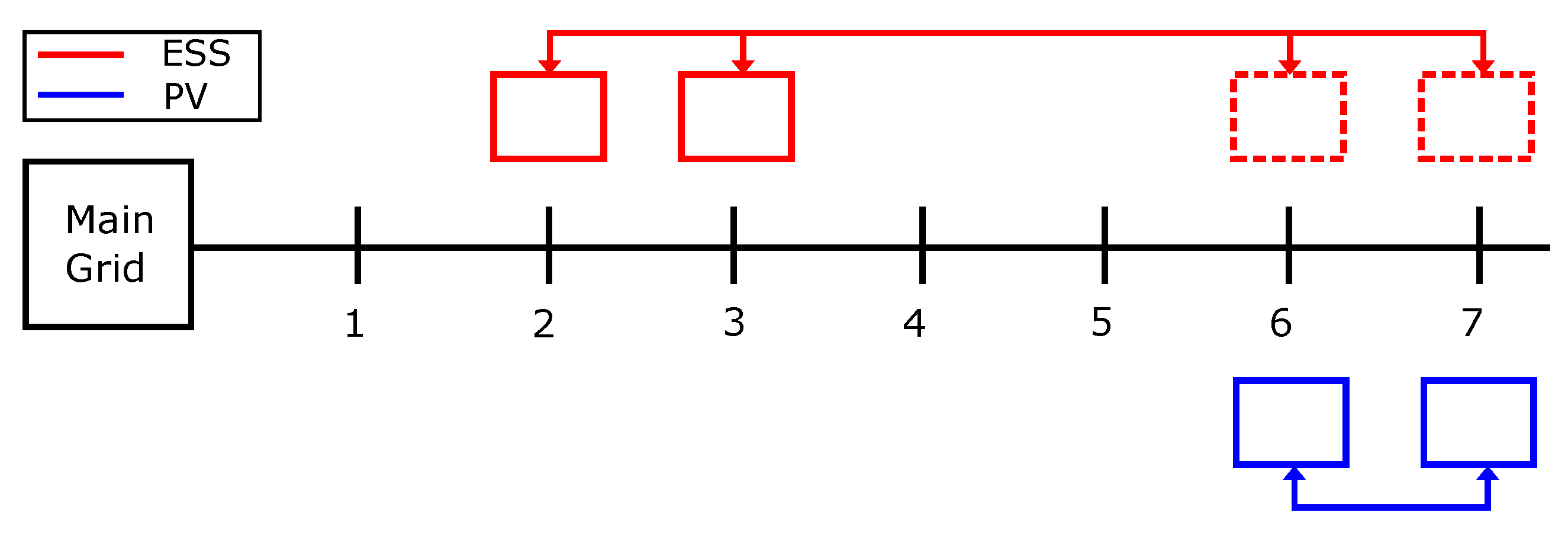
To overcome this issue, in the designed algorithm, the concept of virtual nodes is introduced, which refers to the addition of control nodes that do not actively contribute to the voltage regulation but that participate in the overall control strategy by sharing their multipliers with the rest of the resources (the ESSs in the example at hand). The idea is to add virtual nodes in all the nodes where the DG is present but no ESSs are installed (as shown in Figure 3), since these are the nodes where the maximum overvoltages can be found. These virtual nodes can be seen as additional controllers that have limits on their minimum and maximum power set to zero (namely, $\Delta p_{h_{min}}^{ESS}=\Delta p_{h_{max}}^{ESS}=0$). These virtual nodes do not apply any control output but they exchange Lagrangian multipliers with the other controllers associated to existing ESSs, allowing in this way to involve the ESSs in the control process when an overvoltage is present in the grid.

4. Simulation Setup

This Section provides the overview of the simulated scenario and input data used for the following tests presented in Section 5.

4.1. Distribution Grid

Simulations have been performed on the 23-bus radial LV grid shown in Figure 4, which was taken from the real distribution grid scenario presented in Reference [20].

Table 1. LV distribution grid data.

ID	Start Node	End Node	Per Unit Resistance	Per Unit Reactance	Node ID	No. Customers
01	1	2	0.0004	0.003172	2	0
02	2	3	0.00108675	0.0004095	3	2
03	3	4	0.000426938	0.000160875	4	1
04	4	5	0.00087975	0.0003315	5	1
05	5	6	0.0009315	0.000351	6	1
06	3	7	0.001358438	0.000511875	7	2
07	7	8	3.88125E-05	0.000014625	8	6
08	7	9	0.000685688	0.000258375	9	1
09	7	10	0.00098325	0.0003705	10	3
10	7	11	0.000711563	0.000268125	11	3
11	10	12	0.00098325	0.0003705	12	2
12	10	13	0.0007245	0.000273	13	4
13	13	14	0.000414	0.000156	14	2
14	11	15	0.000905625	0.00034125	15	1
15	15	16	0.000802125	0.00030225	16	2
16	15	17	0.000336375	0.00012675	17	3
17	17	18	0.000659813	0.000248625	18	1
18	18	19	0.000530438	0.000199875	19	2
19	19	20	0.000815063	0.000307125	20	5
20	20	21	0.000336375	0.00012675	21	2
21	21	22	0.00025875	0.0000975	22	4
22	22	23	0.000452813	0.000170625	23	4

shows the impedance data used for the lines, together with the number of customers considered at each node. In the presented simulations, each customer is supposed to be equipped with both a PV plant and an ESS as default scenario. The equivalent power injection/consumption at the nodes is the aggregated power resulting from the contribution of each subtended customer, which will vary depending on the specific load profile, PV generation and ESS charging/discharging behaviour. More details on the generation of the load and PV generation data are provided in the following.

4.2. Load Data

To generate realistic LV load consumption patterns, a tool able to generate stochastic power profiles of residential end-users has been used. The used tool allows emulating the realistic behaviour of residential loads by aggregating the power consumption profiles of single home appliances and considering the statistical information about the probability and time of usage of such appliances, also depending on the time of the season and the yearly energy consumption of the consumers. In this way, the highly intermittent and fluctuating power profiles typically present in the distribution grid can be reproduced and used to test the control algorithms against as realistic as possible scenarios. For the simulations presented in this paper, the profiles for each consumers were randomly generated considering a nominal power of $3.5\mathrm{k}\mathrm{W}$ and a yearly energy consumption of $3500\mathrm{k}\mathrm{W}\mathrm{h}/$year. The created profiles refer to a generic weekday of the summer. Figure 5 shows, as an example, the daily load profile resulting from the aggregation of the connected consumers for some of the grid nodes.

4.3. PV Data and Model

The generation profiles used to emulate the PV production have been created using the PV profiles generator presented in Reference [28]. This tool allows reproducing daily profiles of PV generation for different locations, days of the year, and PV installation characteristics (e.g., azimuth angle, tilt angle, etc.). Moreover, the software offers the possibility to consider also varying weather conditions, thus emulating the resulting impact of different cloudiness levels on the irradiance and, consequently, on the generated active power. Thanks to these features, the PV generator tool gives the possibility to create clear sky generation profiles, which can be used to test “worst case scenarios” where all the PV plants produce their maximum active power, thus turning into the most critical situation for the occurrence of the overvoltage. At the same time, the tool also allows creating fluctuating profiles associated to possible cloudy weather conditions, which can be used to test the efficacy of the control algorithm in presence of highly intermittent generation, thus taking into account a realistic scenario that is likely to occur in the daily operation of the distribution grid.

In the simulations presented in the next Section, all the customers are supposed to have a PV plant with a nominal power of $4\mathrm{k}\mathrm{W}$. Figure 6 shows the detail of the generation profiles under clear sky and cloudy conditions created for the following tests. The generation profiles shown for each node are cumulative, meaning that they are the aggregation of the PV generation for all the customers connected to the node. The generation profiles refer to a day in August and have been created by considering N50°77′ E6°9′ (coordinates corresponding to the city of Aachen, in Germany) as location of the distribution grid and assuming, for the sake of simplicity, that all the PV plants have the same azimuth angle equal to ${180}^{°}$ degrees and a tilt angle equal to ${30}^{°}$ degrees.

5. Simulation Results

The optimization algorithm presented in Section 3 has been implemented in Python and it has been tested in loop with a power flow simulation of the grid [29]. Simulations have been performed to validate the proposed coordinated control of ESSs and DG in different scenarios and to compare this control strategy with a solution where only DG is involved. The code used for the simulations is available online and freely downloadable [30].

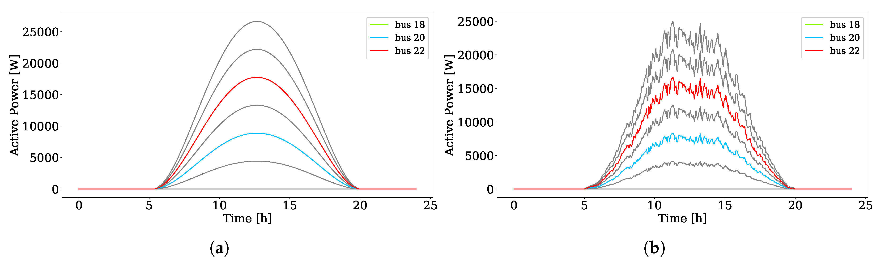
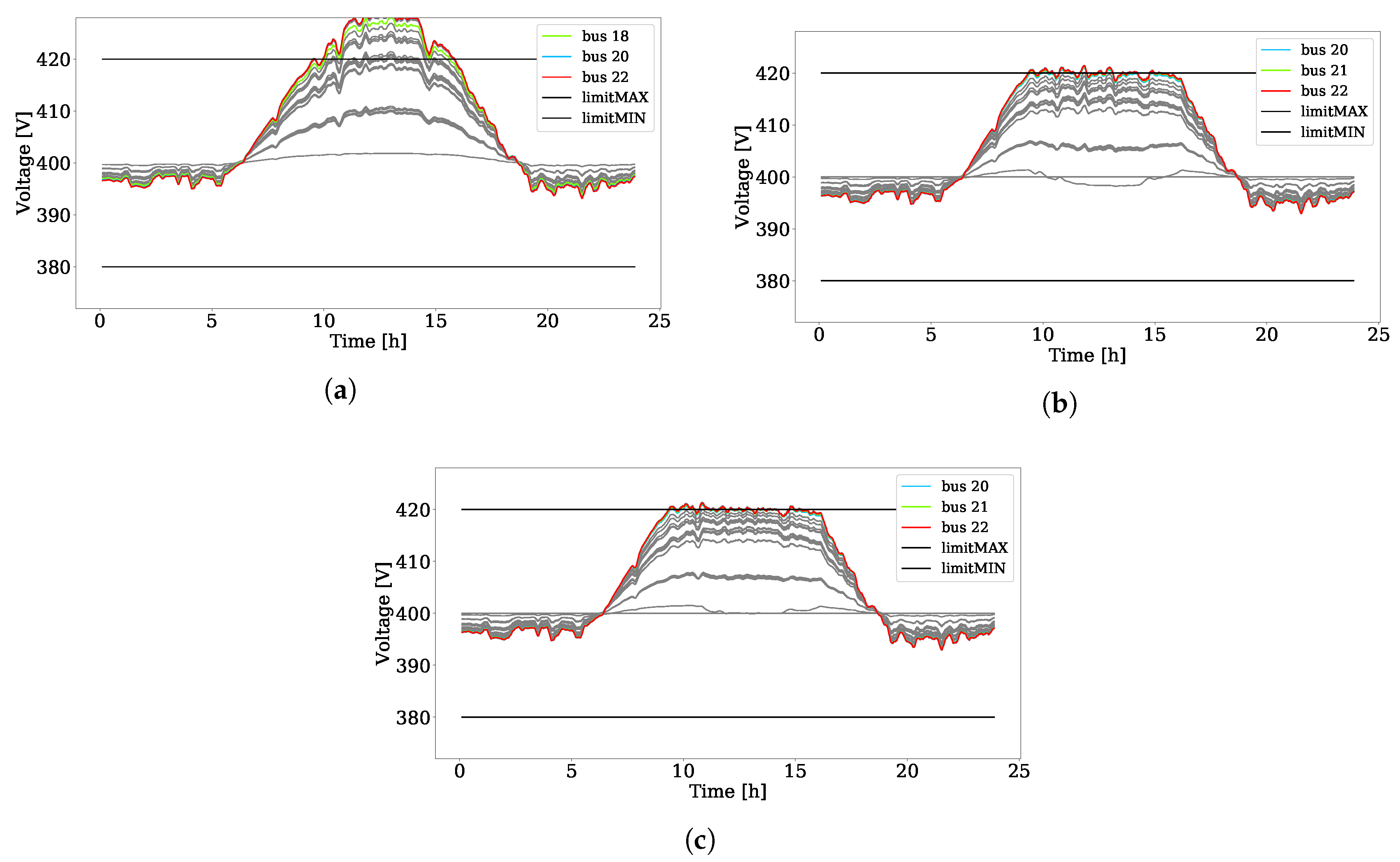
A first test has been performed considering a worst case scenario with high PV generation obtained in presence of clear sky conditions. Figure 7a shows the effect of the high penetration of the renewable generation in a totally uncontrolled scenario, which leads to an overvoltage condition for a considerable number of grid nodes (in grey color the grid nodes not in the legend) and for a significant interval of time during the central part of the day. On the contrary, Figure 7b,c (which refer to the case of control performed only with DG or involving both DG and ESSs, respectively) clearly highlight the beneficial effect brought by the implementation of the designed voltage control: in fact, in both the scenarios the voltage profiles remain within the allowed limits.

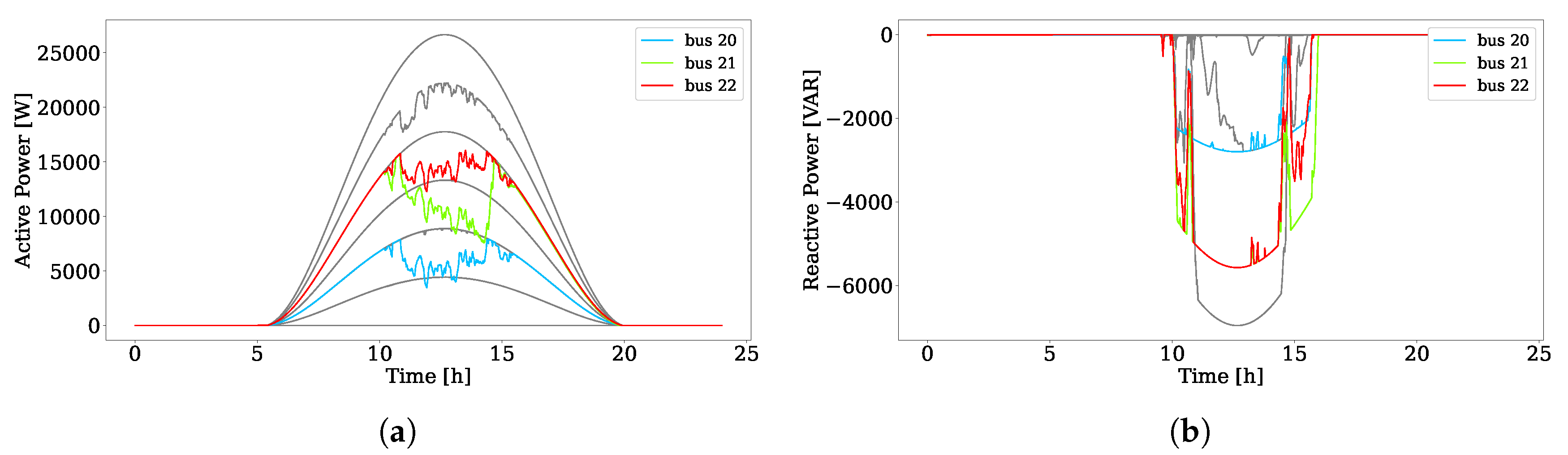
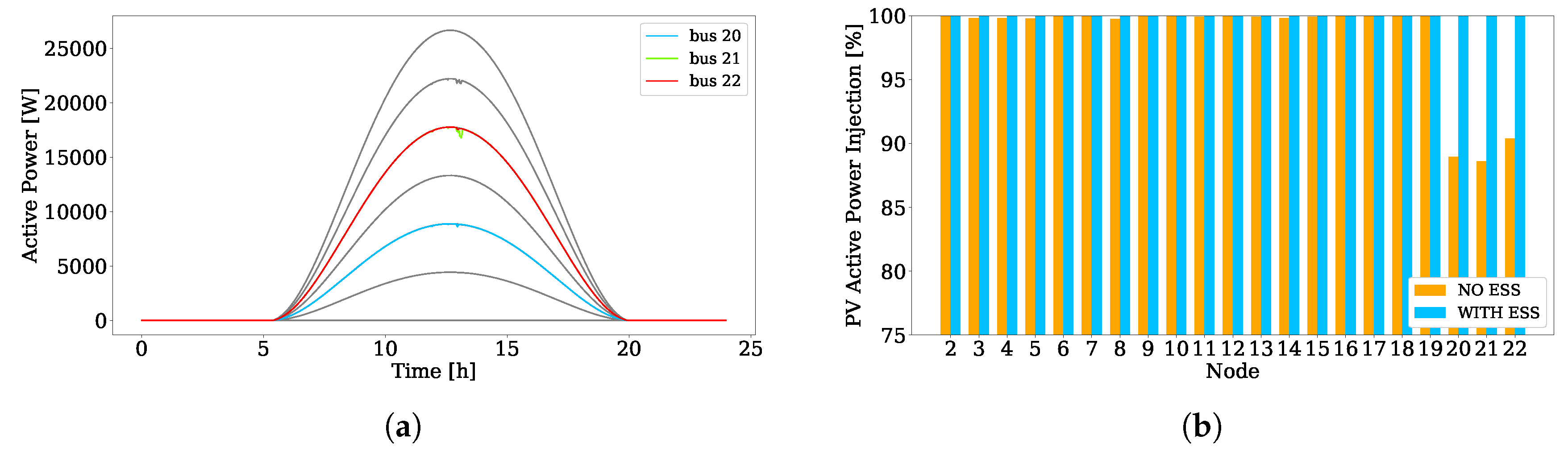
While the effects of the control applied only to the DG or to both DG and ESSs are similar in terms of obtained voltage profile, some important differences can be observed when looking at the resulting power profiles of the PV. Figure 8 shows the active power injected and the reactive power absorbed by the PVs in the case where only the DG is considered for the voltage control. These figures highlight that in the considered scenario, the PV active power control is activated in some nodes because the reactive power absorption has reached its limit, meaning that the corresponding Lagrangian multipliers became different from zero and therefore the logic managing the PV active power control reacted to modify the values of the parameter ${\alpha }_P$ in order to enable the active power curtailment. As visible in Figure 8a, the active power injected by the PVs is consequently reduced in some of the nodes (e.g., nodes 20, 21 and 22) during the central hours of the day, since the reactive power absorption was not sufficient in that moment of the day to compensate for the overvoltage. Obviously, this automatically translates into the waste of potentially available clean energy as well as in additional system costs if the DSO is called to pay for compensating the customers affected by the loss of generated power.

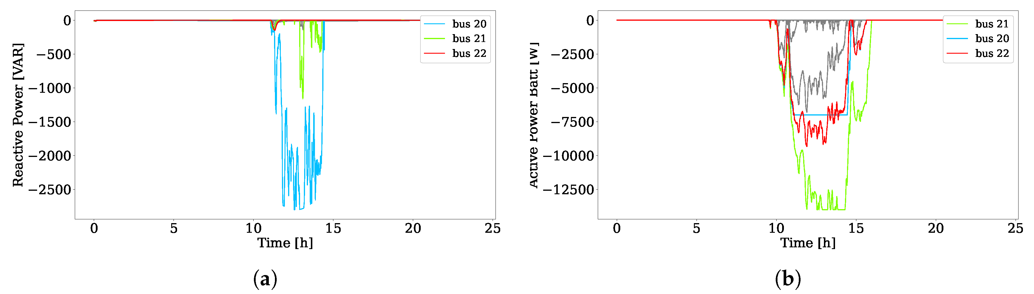
Figure 9 describes instead the case where the control of the ESSs is also additionally applied. As discussed in Section 3.4, an important feature of the proposed coordinated voltage control algorithm is the possibility to flexibly decide the contribution of the different resources to the voltage rise mitigation. In particular, this can be done by tuning the parameters $\alpha$ used within the control algorithm. While this paper does not aim at establishing optimal rules for the definition of the values of these parameters, tests have been performed to assess the possible impact of a different selection of such setting. In this regard, Figure 10 shows the results deriving from the application of the logic presented in Section 3.4, where the charging of active power in the ESSs is prioritized with respect to the absorption of reactive power from the DG. As a result of this prioritization logic, it is possible to observe that the values of active power values provided to the ESSs reach the available limits for some of the nodes, meaning that the associated ESSs charge at their maximum power. In this case, it is possible to observe that the number of PVs reaching the limit of reactive power consumption is smaller, and this consequently reduces also the amount of curtailed active power (as visible from the comparison between Figure 8a and Figure 9a). The corresponding active power absorbed by the ESSs (operation in charging mode) is given in Figure 10b. It shows that, like for the reactive power control, the control algorithm provides control set-points to absorb active power as soon as the node voltages reach the upper limit. 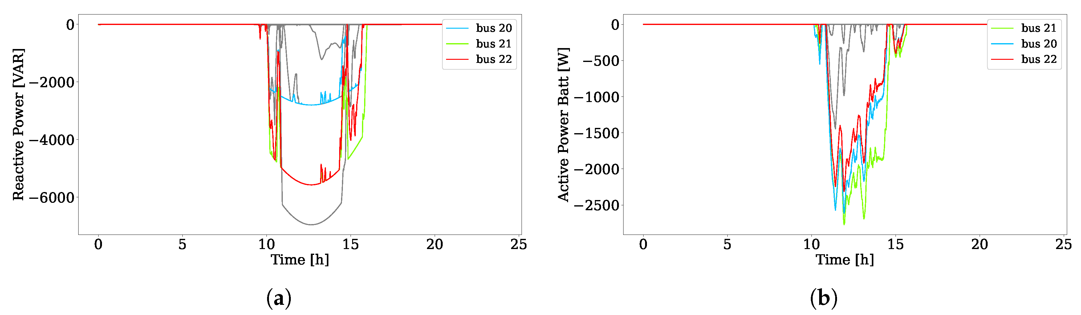As described in Section 3.4, DGs reactive power control could also be prioritized with respect to the active power control of the ESSs. The result of this prioritization strategy is described in Figure 11, where it is clear that the amount of reactive power increased and the active power of the ESSs decreased compared to the above scenario. Since the active power curtailment is activated only when reactive power of PVs and active power of ESSs of a set of neighbors reach the limit, a change in the prioritization scheme does not modify the curtailment of the active power.

The results of the three different simulation tests are summarized in

Table 2. Summary of the simulation tests.

Case	Reactive Power Injection PVs (kVAR)	Active Power Curtailment PVs (kW)	Active Power Injections ESSs (kW)
No ESSs	−4.3	−2.1	0.0
ESSs priority	−0.3	0.0	−5.5
PVs priority	−4.4	0.0	−2.0

, where reactive power injections and active power injections for each customers are averaged over the number of data points collected. The Table demonstrates the positive impact of the coordinated control on reducing the active power curtailment in both ESS and PV prioritization.

As described in Section 2.3, a goal of this work is to assess the impact of coordinating the ESSs charging and the DG reactive power provision for mitigating the overvoltage events occurring in the distribution grid. Therefore, the active power charging behaviour of the batteries does not follow any customer-based profile and it is set to zero when no overvoltages are present. This approach, although not combined with independent charging/discharging profiles, helps understanding the sole contribution of the ESSs to limit the voltage rise. The advantage of integrating the ESSs in the voltage control strategy is shown in Figure 10b, where the curtailment of active power injected by the PVs is presented for the two cases of control with and without the ESSs. More specifically, Figure 10b provides the percentage of PV energy provided by each node over the day in the two control options previously described. The comparison of the results, while strictly related to the specific scenario under test, clearly demonstrates the potential advantage achievable, when using the ESSs, in terms of reduction of the active power curtailment. This is emphasized especially for the nodes at the end of the feeders of the grid, where the effects of the voltage rise are more evident.

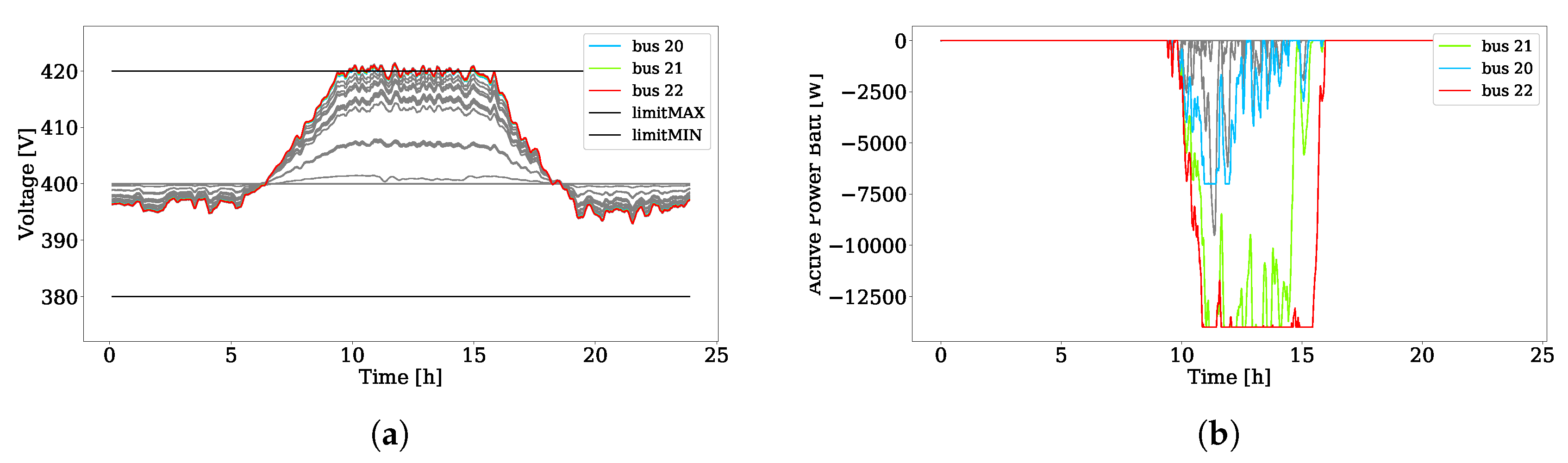
Additional tests have been conducted considering the PV profiles described in Section 4.3 emulating a day with cloudy conditions. While this case is not the worst one in terms of resulting overvoltage, it is important to assess the behaviour of the optimization algorithm in this scenario, since the highly dynamic and fluctuating conditions of the voltage and power profiles could affect the expected operation of the control. Figure 12a highlights that, also in this scenario, the capabilities of the coordinated control to maintain the voltage within the allowed boundaries are not affected by the stochastic behaviour of the DG. At the same time, however, Figure 12b also shows that the desired voltage output is achieved at the expenses of a very highly fluctuating profile of the ESS charging. This could highlight the need to take adequate countermeasures in the control strategy in the case in which constraints exist for the maximum variations that can be applied to the charging/discharging power profile of the ESS.

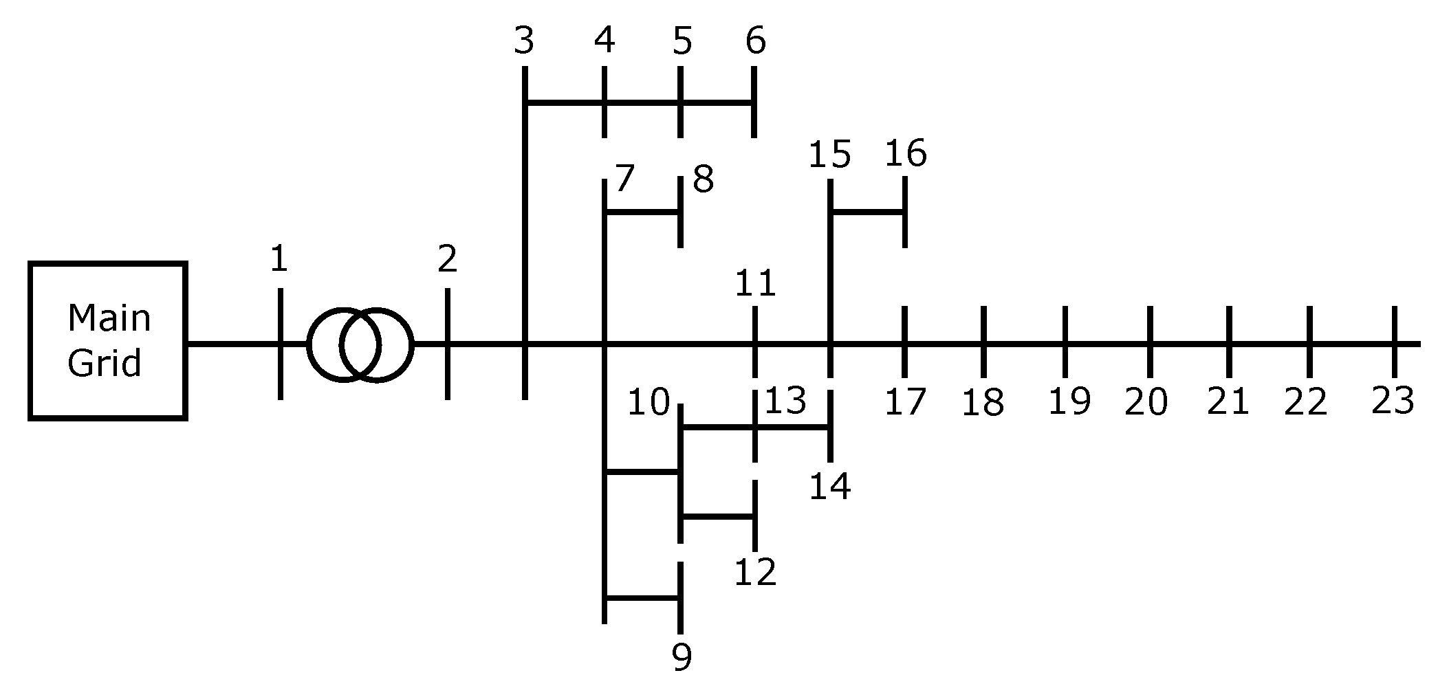
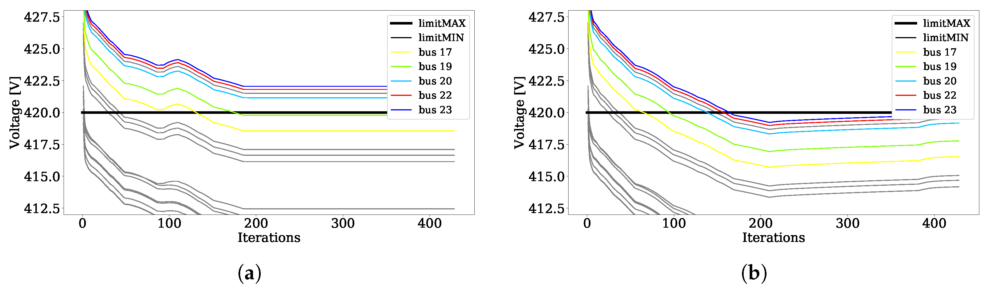
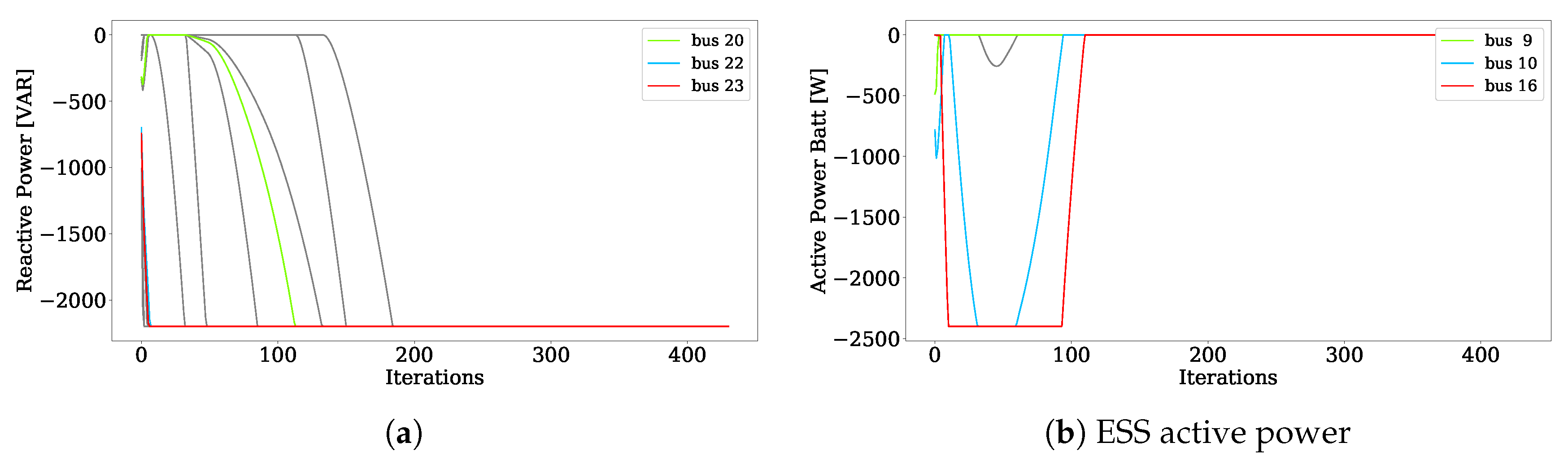
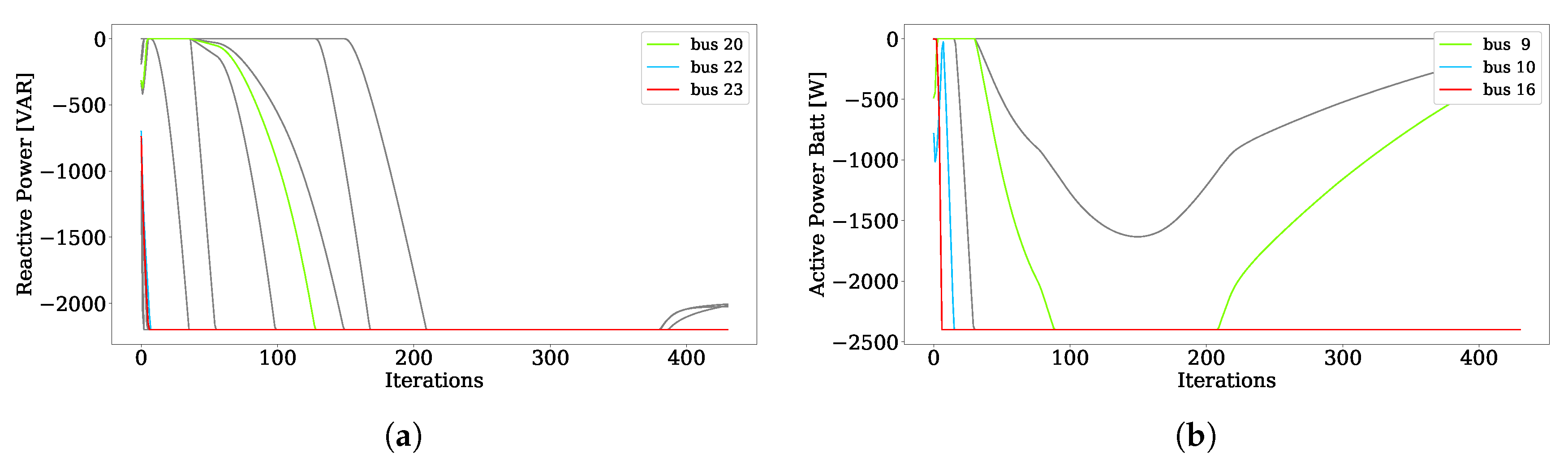
Another set of simulations has been performed to prove the key role played by the introduction of the virtual nodes for the effective coordination of the DG and ESS control. The test here presented consists of a scenario where each load has a constant active power consumption of $1\mathrm{k}\mathrm{W}$ and the installed PVs have active power generation of $8\mathrm{k}\mathrm{W}$. The PV generators are placed in nodes $N_{DG}=[5,6,7,8,9,13,14,15,16,17,19,20,22,23]$ whereas the ESSs have been arbitrarily placed in $N_{ESS}=[4,5,6,7,10,11,17]$, to emulate a generic scenario where PVs and ESSs are not placed in the same locations. In this configuration, overvoltages arise at the last nodes of the grid and consequently the reactive power control activates to decrease the voltage levels. If virtual nodes are not used, since the voltage values from node 1 to 19 are below the limit, the active power control of the ESSs is not activated. As shown in Figure 13a, this can lead to cases where the overvoltage is not solved if the DG active power curtailment is not activated (in this set of simulations the DG active power control has been disabled to allow an easier comparison of the results for the cases with or without virtual nodes). On the other hand, the same overvoltage situation can be solved, without using any renewable generation curtailment, exploiting instead the available ESSs resources, if virtual nodes are introduced. To this purpose, virtual nodes have been added to nodes $N_{ESS}=[19,20,22,23]$, namely in those nodes where PVs without ESSs are installed. As visible in Figure 13b, with this set-up, the proposed control algorithm is able to handle the overvoltage and to bring the voltage magnitude within the allowed thresholds for all the nodes of the grid. As explained in Section 3.5, the virtual nodes do not actively contribute to the reduction of the voltage values but they make the ESSs aware of the overvoltage by sharing their Lagrangian multipliers. This allows activating the absorption of active power by the ESSs also in the nodes where the overvoltage is not present (see the comparison between the power profiles in Figure 14 and Figure 15), leading to a proper reduction of the voltage also in the last nodes of the grid.

6. Conclusions

This paper presented the design of a coordinated control for overvoltage mitigation in distribution grids. The proposed distributed control strategy aims at controlling the active and reactive power of DGs as well as the active power of the ESSs, thus allowing fully exploiting the resources potentially available in the grid. Numerical simulations on a sample LV grid have been performed to assess the performance of the designed control. Test results prove that the proposed control strategy is able to guarantee the operation of the network within the permitted voltage boundaries and that the coordinated use of ESSs and DG allows reducing the needs for active power generation curtailments. The performance of the control algorithm can be further refined by applying a smart tuning of some of the optimization parameters, which are directly correlated to the level of participation of each resource to the overall overvoltage mitigation action. Moreover, performed tests also prove the robustness of the proposed control method against typical intermittent and fluctuating profiles of load and generation, which are often found at distribution level. The concept of virtual nodes has been introduced and tested, demonstrating that the coordination among the resources distributed in the grid can be improved by adding additional control nodes that, although not controlling directly a physical device, can contribute to the overall voltage control. Overall, the active coordination of ESSs and DG by means of the proposed voltage control algorithm allows fulfilling the primary goal of maintaining the voltage within the desired boundaries, while relying on a relatively simple implementation of the control logic that can be distributed locally among the available resources in the grid. Thus, such control technique can be an interesting option for enabling the real-time voltage control of the grid and to allow a larger integration of renewable energy sources in the system, above all at low voltage level, where currently it is rare to find central energy management systems running a centralized control. The proposed solution could be directly embedded in the control logic of DG and ESSs, thus not requiring the installation of any additional physical devices. The proposed control scheme is an interesting option also to allow a larger penetration of DG in low voltage grids without requiring additional investments on the phyisical assets of the grid. This solution could be thus attractive for DSOs in the next future, thanks to the upcoming regulation changes aimed at incentivizing the investments in software-based smart solutions.

References

1. Von Appen, J.; Braun, M.; Stetz, T.; Diwold, K.; Geibel, D. Time in the sun: The challenge of high PV penetration in the German electric grid. IEEE Power Energy Mag. 2013, 11, 55–64. [Google Scholar] [CrossRef]
2. Ferreira, P.D.; Carvalho, P.M.; Ferreira, L.A.; Ilic, M.D. Distributed energy resources integration challenges in low-voltage networks: Voltage control limitations and risk of cascading. IEEE Trans. Sustain. Energy 2013, 4, 82–88. [Google Scholar] [CrossRef]
3. Navarro-Espinosa, A.; Ochoa, L.F. On the cascading effects of residential-scale PV disconnection due to voltage rise. In Proceedings of the 2014 IEEE PES General Meeting| Conference & Exposition, Washington, DC, USA, 27 July 2014; pp. 1–5. [Google Scholar]
4. Resch, M.; Buehler, J.; Klausen, M.; Sumper, A. Impact of operation strategies of large scale battery systems on distribution grid planning in Germany. Renew. Sustain. Energy Rev. 2017, 74, 1042–1063. [Google Scholar] [CrossRef] [Green Version]
5. Bayer, B.; Matschoss, P.; Thomas, H.; Marian, A. The German experience with integrating photovoltaic systems into low-voltage grids. Renew. Energy 2018, 119, 129–141. [Google Scholar] [CrossRef]
6. Mutale, J. Benefits of Active Management of Distribution Networks with Distributed Generation. In Proceedings of the 2006 IEEE PES Power Systems Conference and Exposition, Atlanta, GA, USA, 5 February 2006; pp. 601–606. [Google Scholar]
7. Stetz, T.; Marten, F.; Braun, M. Improved low voltage grid-integration of photovoltaic systems in Germany. IEEE Trans. Sustain. Energy 2012, 4, 534–542. [Google Scholar] [CrossRef]
8. European Commission. Do Current Regulatory Frameworks in the EU Support Innovation and Security of Supply in Electricity and Gas Infrastructure? Final Report European Commission. 2019. Available online: https://ec.europa.eu/info/sites/info/files/reportregulatoryfw.pdf (accessed on 16 April 2020).
9. Turitsyn, K.; Sulc, P.; Backhaus, S.; Chertkov, M. Local control of reactive power by distributed photovoltaic generators. In Proceedings of the 2010 First IEEE International Conference on Smart Grid Communications, Gaithersburg, MD, USA, 4–6 October 2010; pp. 79–84. [Google Scholar]
10. Farivar, M.; Zho, X.; Che, L. Local voltage control in distribution systems: An incremental control algorithm. In Proceedings of the 2015 IEEE International Conference on Smart Grid Communications (SmartGridComm), Miami, FL, USA, 5 November 2015; pp. 732–737. [Google Scholar]
11. Bolognani, S.; Carli, R.; Cavraro, G.; Zampieri, S. On the Need for Communication for Voltage Regulation of Power Distribution Grids. IEEE Trans. Control Netw. Syst. 2019, 6, 1111–1123. [Google Scholar] [CrossRef]
12. Antoniadou-Plytaria, K.E.; Kouveliotis-Lysikatos, I.N.; Georgilakis, P.S.; Hatziargyriou, N.D. Distributed and decentralized voltage control of smart distribution networks: Models, methods, and future research. IEEE Trans. Smart Grid 2017, 8, 2999–3008. [Google Scholar] [CrossRef]
13. Brenna, M.; De Berardinis, E.; Delli Carpini, L.; Foiadelli, F.; Paulon, P.; Petroni, P.; Sapienza, G.; Scrosati, G.; Zaninelli, D. Automatic Distributed Voltage Control Algorithm in Smart Grids Applications. IEEE Trans. Smart Grid 2013, 4, 877–885. [Google Scholar] [CrossRef]
14. Bottura, R.; Borghetti, A. Simulation of the Volt/Var control in distribution feeders by means of a networked multiagent system. IEEE Trans. Ind. Inf. 2014, 10, 2340–2353. [Google Scholar] [CrossRef]
15. Zhang, B.; Lam, A.Y.; Domínguez-García, A.D.; Tse, D. An optimal and distributed method for voltage regulation in power distribution systems. IEEE Trans. Power Syst. 2014, 30, 1714–1726. [Google Scholar] [CrossRef] [Green Version]
16. Bolognani, S.; Zampieri, S. A distributed control strategy for reactive power compensation in smart microgrids. IEEE Trans. Automatic Control 2013, 58, 2818–2833. [Google Scholar] [CrossRef] [Green Version]
17. Molzahn, D.K.; Dörfler, F.; Sandberg, H.; Low, S.H.; Chakrabarti, S.; Baldick, R.; Lavaei, J. A survey of distributed optimization and control algorithms for electric power systems. IEEE Trans. Smart Grid 2017, 8, 2941–2962. [Google Scholar] [CrossRef]
18. Palensky, P.; Dietrich, D. Demand side management: Demand response, intelligent energy systems, and smart loads. IEEE Trans. Ind. Inf. 2011, 7, 381–388. [Google Scholar] [CrossRef] [Green Version]
19. Von Appen, J.; Stetz, T.; Braun, M.; Schmiegel, A. Local voltage control strategies for PV storage systems in distribution grids. IEEE Trans. Smart Grid 2014, 5, 1002–1009. [Google Scholar] [CrossRef]
20. Hashemi, S.; ∅stergaard, J. Efficient control of energy storage for increasing the PV hosting capacity of LV grids. IEEE Trans. Smart Grid 2016, 9, 2295–2303. [Google Scholar] [CrossRef] [Green Version]
21. Zarrilli, D.; Giannitrapani, A.; Paoletti, S.; Vicino, A. Energy storage operation for voltage control in distribution networks: A receding horizon approach. IEEE Trans. Control Syst. Technol. 2017, 26, 599–609. [Google Scholar] [CrossRef]
22. Farivar, M.; Chen, L.; Low, S. Equilibrium and dynamics of local voltage control in distribution systems. In Proceedings of the 52nd IEEE Conference on Decision and Control, Florence, Italy, 15 May 2013; pp. 4329–4334. [Google Scholar]
23. CENELEC. EN 50160: Voltage Characteristics of Electricity Supplied by Public Electricity Networks; CENELEC: Brussels, Belgium, 2010. [Google Scholar]
24. VDE. Erzeugungsanlagen am Niederspannungsnetz, Technische Mindestanforderungen für Anschluss und Parallelbetrieb von Erzeugungsanlagen am Niederspannungsnetz; VDE-AR-N4105; VDE: Frankfurt, Germany, 2011. [Google Scholar]
25. Magnússon, S.; Qu, G.; Fischione, C.; Li, N. Voltage control using limited communication. IEEE Trans. Control Netw. Syst. 2019, 993–1003. [Google Scholar] [CrossRef] [Green Version]
26. Bertsekas, D.P. Nonlinear programming. J. Operat. Res. Soc. 1997, 48, 334. [Google Scholar] [CrossRef]
27. Bolognani, S.; Carli, R.; Cavraro, G.; Zampieri, S. Distributed reactive power feedback control for voltage regulation and loss minimization. IEEE Trans. Automatic Control 2015, 60, 966–981. [Google Scholar] [CrossRef] [Green Version]
28. Pau, M.; Angioni, A.; Ponci, F.; Monti, A. A Tool for the Generation of Realistic PV Profiles for Distribution Grid Simulations. In Proceedings of the 2019 International Conference on Clean Electrical Power (ICCEP), Otranto, Italy, 2 July 2019; pp. 193–198. [Google Scholar]
29. PYPOWER. Available online: https://pypi.org/project/PYPOWER/ (accessed on 16 April 2020).
30. Code Algorithms. Available online: https://git.rwth-aachen.de/acs/public/publications/de-din-coordinated-voltage-control (accessed on 16 April 2020).
Figure 1. Example 3-bus system.
Energies 13 02007 g001
Figure 2. LV grid without virtual nodes.
Energies 13 02007 g002
Figure 3. LV grid with virtual nodes.
Energies 13 02007 g003
Figure 4. LV Distribution Network.
Energies 13 02007 g004
Figure 5. Example of load profiles for some of the nodes of the grid.
Energies 13 02007 g005
Figure 6. Generated PV profiles for clear sky and cloudy weather conditions. (a) Photovoltaic (PV) profiles under clear sky conditions. (b) PV profiles under cloudy conditions.
Energies 13 02007 g006
Figure 7. Voltage profile of the grid for different control strategies under clear sky conditions. (a) No control (b) Only DG control (c) Both DG and ESSs control.
Energies 13 02007 g007
Figure 8. Distributed control applied only to DG. (a) Active power generated by PVs (b) Reactive power generated by PVs.
Energies 13 02007 g008
Figure 9. Distributed control applied to both Distributed Generation (DG) and Energy Storage Systems (ESSs). (a) Active power generated by PVs (b) Percentage level of PV energy production.
Energies 13 02007 g009
Figure 10. ESS power and DG energy production with prioritized use of the ESS over the DG. (a) Reactive Power generated by PVs. (b) Active power injected by ESSs.
Energies 13 02007 g010
Figure 11. ESS power and DG reactive power with prioritized use of the DG over the ESS. (a) Reactive power generated by PVs. (b) Active power injected by ESS.
Energies 13 02007 g011
Figure 12. Results for the designed control strategy under cloudy sky conditions. (a) Voltage profile. (b) Active power injected by ESS.
Energies 13 02007 g012
Figure 13. Voltage profile without virtual nodes and with virtual nodes. (a) Without virtual nodes (b) With virtual nodes.
Energies 13 02007 g013
Figure 14. DG and ESS power injection in scenario without virtual nodes. (a) DG reactive power (b) ESS active power.
Energies 13 02007 g014
Figure 15. DG and ESS power injection in scenario with virtual nodes. (a) DG reactive power (b) ESS active power.
Energies 13 02007 g015