Abstract
For many years, primary weather forecasting services (Global Forecast System (GFS) and the European Centre for Medium-Range Weather Forecasts (ECMWF)) have been made available to the public through global Numerical Weather Prediction (NWP) models estimating a multitude of general weather variables in a variety of resolutions. Secondary services such as weather experts Meteomatics AG use data and improve the forecasts through various methods. They tailor for the specific needs of customers in the wind and solar power generation sector as well as data scientists, analysts, and meteorologists in all areas of business. These auxiliary services have improved performance and provide reliable data. However, this work extended these auxiliary services to so-called tertiary services in which the weather forecasts were further conditioned for the very niche application environment of mobile solar technology in solar car energy management. The Gridded Model Output Statistics (GMOS) Global Horizontal Irradiance (GHI) model developed in this work utilizes historical data from various ground station locations in South Africa to reduce the mean forecast error of the GHI component. An average Root Mean Square Error (RMSE) improvement of 11.28% was shown across all locations and weather conditions. It was also shown how the incorporation of the GMOS model could have increased the accuracy in regard to the State of Charge (SoC) energy simulation of a solar car during the Sasol Solar Challenge 2018 and the possible range benefits thereof.
1. Introduction
Solar technology is becoming popular for use on car roofs to increase the drivable range. Automotive giants such as Toyota (Toyota City, Japan) and Hyundai (Seoul, South Korea) are incorporating this technology and claim noteworthy range extension [1]. Cars developed for an urban specific use such as the Squad car from Squad Mobility (Amsterdam, Netherlands) and Sion from Sono Motors (München, Germany) [2] claim a range of over 20 km per day on solar power alone. Others, such as the Lightyear One (Helmond Netherlands) solar car, is capable of doing up to 72 km on solar power alone and 725 km when combined with a battery [3]. Some niche area solar car development is ongoing mainly in the academic environment among Engineering students. Here teams are challenged to design light-weight, single-seater solar-powered vehicles capable of driving on national motorways for thousands of kilometers over a few days without ever re-charging with grid energy [4]. These niche endurance challenges exploit the massive energy potential emitted by the sun, one of the few remaining renewable energy resources on our planet. The two most prominent solar endurance challenges are the Bridgestone World Solar Challenge in Australia (BWSC) and the Sasol Solar Challenge in South Africa (SSC). These solar-powered electric cars all have one common denominator, the sun. The amount of solar irradiance from the sun and its availability (clouds, air quality, etc.) directly affects the performance of these solar-powered electric vehicles.
An integral part of ensuring an accurate energy model, specifically solar-powered electric vehicles, is by including relevant weather conditions to the energy model. Knowing what the weather conditions might be before traveling a particular route will be beneficial to be able to plan such a route effectively. For example, a commuter might be planning to drive the following morning to a town 300 km away from his current location (the range of this solar electric vehicle is 300 km with good sunshine when traveling at 120 km/h). He is not aware that the weather forecast until 13:00 the next day predicts fully overcast conditions (which would force the driver to drive slower to conserve energy). The commuter will surely become frustrated when departing early while having to drive slowly rather than leaving after lunch and being able to drive at a good pace. One can then argue that if the driver had to watch the weather channel the previous day, they would have been able to make the necessary adjustments to their trip. However, when you have to consider the clouds, wind speed and direction, the air density, the solar irradiance forecast, and the variability of these parameters (risk in the forecasts), it quickly becomes apparent and somewhat necessary to make the weather forecasts more accurate, refined, and used in context to become more useful for a vehicle energy model. The solar irradiance forecast is by far the most influential of all the weather parameters in the context of solar-powered electric vehicles.
The SSC is a biennial challenge where teams from around the globe design and build solar-powered vehicles to compete in an eight-day event spanning South Africa. Local and international solar-powered cars drive as far as they can on motorways between Pretoria and Cape Town. Pre-defined additional detours are allowed each day to maximize distance; however, the stopover locations for each night are fixed. The challenge aims to achieve the maximum distance while adhering to the event constraints as well as the local road and safety rules. Some teams make use of computer simulations to optimize their speed for minimum energy usage. These simulations make use of an extensive mathematical model describing the aerodynamic, rolling resistance as well as gravitational behavior of the car while in motion. Most of the variables contained in these mathematical functions are deterministic and reasonably trivial to calculate, measure, or approximate [5]. Another input to these energy simulations is the local weather forecast and one such forecast variable which is of great concern, the Global Horizontal Irradiance (GHI). The solar panels on a solar car are predominantly mounted in a horizontal orientation; hence, the GHI is the most appropriate solar irradiance quantity to use as this quantifies the amount of solar radiation falling on a horizontal plane relative to the ground. The amount of GHI reaching the earth’s surface is affected by various other variables. However, the most significant contributor is the amount of Total Cloud Cover (TCC). The TCC is the fraction of the sky covered (or hidden) by all the visible clouds [6].
Two prominent databases are available which supply weather forecasts to the public for general use. The European Centre for Medium-Range Weather Forecasts Integrated Forecasting System (ECMWF-IFS) [7] and the Global Forecast System (GFS) [8] produced by the National Centers for Environmental Prediction. These two global databases provide a wide range of meteorological forecasts. Although these forecast providers offer reliable and readily available data, a need arose for intermediary (secondary) services that take data from these sources and apply some techniques to improve the accuracy and reliability. Many of these intermediary weather services exist [9] and are used by energy managers for solar installations, wind installations, meteorologists, sailors, farmers, weather enthusiasts, and many more. Recently, the forecasts that these secondary services provide has also become essential to participants of solar-powered electric vehicle teams in events such as the BWSC in Australia and the SSC in South Africa. Many researchers are now taking this intermediary forecast data and refining even further (tertiary) by combining with some historical data, creating forecast ensembles, or applying some regression methods. This is in an attempt to make the forecast data even more useful for specialized local applications in a variety of areas [10]. For this work, the focus will be placed on the raw forecasts provided by a secondary service, Meteomatics AG (experts in weather processing and forecasting, based in Gallen, Switzerland), who makes use of the ECMWF as a primary data source.
An extensive forecasting technique comparison has been made [11], and the best forecast techniques were found to be Artificial Neural Network (ANN) based methods. This work, however, only shows results for one day ahead forecasting, and the process of training the ANN is relatively lengthy and intricate and requires seven other weather variables apart from GHI and TCC to train. Furthermore, the work does not apply the forecasting techniques to a real-world application to show how improved accuracy can lead to an increase in application performance. Other techniques such as Model Output Statistics (MOS) has been used since 1972 [12] for site-specific forecasts. MOS is a post-processing forecast method that uses data of some predictand (such as the GHI forecast) and relates to some historical statistical data of some other predictors (such as GHI and TCC). Gridded-MOS [12,13], or GMOS, is an extension of MOS which is created by a whole network of ground observation stations to create a forecast grid model for a larger area. The more ground observation stations in the grid, the better the GMOS model performance will be for the region.
A three-year study in Germany [14] found ECMWF GHI MOS refined forecasts at several thousand photovoltaic plants with an average daily RMSE value of 24.5%. This is compared to raw ECMWF GHI forecasts in Germany at 36% RMSE [15]. The same authors showed how to create forecast confidence intervals and how this can be applied to forecast models. More work on ECMWF GHI MOS models was done at Reunion Island over one year during 2011, and the authors [16] showed an average RMSE reduction of 13%. Similarly, a general reduction in relative RMSE values of GHI forecasts for one-day ahead predictions were found to be 15.1% by researchers in the Netherlands [17]. They made use of raw forecasts by NWP models from the ECMWF as well as the GFS. In Australia [18], the ECMWF GHI prediction accuracy (RMSE) was found to be between 18% to 45% for a one-year sample set and averaged over a five-day forecast horizon. A twelve month comparative study in 2013 [19] on GHI forecasts in the US, Canada, and Europe revealed that the GHI forecast accuracy from NWP models could vary tremendously based on the geographical location. The average raw ECMWF predictions were seen anywhere in the range of 20% to 65% (RMSE) and the average MOS compensated models were seen in the region of 15% to 44% (RMSE). The study also showed a significant reduction in MOS forecast bias by up to 21% less RMSE than the raw ECMWF predictions.
The improvement of the GHI forecast component is essential for route and speed planning, especially with cars relying heavily on solar power such as Lightyear One [3] and the single-seater prototype solar cars designed by teams competing in the BWSC and the SSC. Through a better understanding of the risk associated with the available GHI forecast, the energy manager of the team will be able to make better and more energy-conscious decisions. In the current literature, there is no mention of how a MOS or GMOS model can benefit the teams participating in an SSC event in terms of energy management.
This work aims to improve the State of Charge (SoC) simulation accuracy of an SSC solar car team by using GMOS methods in GHI forecasting along the route of an SSC event in South Africa. The mandatory event route for the SSC 2018 is shown in Figure 1.

Figure 1.
Sasol Solar Challenge (SSC) 2018 route.
2. Materials and Methods
Ground station measured data has been taken from strategic locations along the SSC route. The chosen locations were Pretoria (University of Pretoria), Bloemfontein (Central University of Technology), Port Elizabeth (Nelson Mandela University), and the Cape Town area (Stellenbosch University). The ground station data was obtained from a public data source provided by the Southern African Universities Radiometric Network (SAURAN) [20], in Stellenbosch South Africa, where data for 2018 to the end of 2019 was requested from this public source. This data source stores hourly averaged measured values for a variety of meteorological variables; however, only the GHI and TCC components were of concern for this work.
SAURAN has a total of 23 ground measurement stations across South Africa. The limitation of a maximum allowed daily data point requests (as imposed by the forecast provider Meteomatics AG) limited the Application Program Interface (API) requests to four locations in South Africa only. All four cities are major stopover locations for the SSC event and span the entire route from start to finish. Forecast data was made available by Meteomatics AG. Their forecast data originates from the ECMWF database; however, Meteomatics AG improves the forecast before making it available to its users. An API script was developed and used over two years (2018–2019) to request daily the GHI and TCC forecast for each of the four locations spanning a nine-day horizon. This data was then stored in a multi-dimensional matrix format (Matlab by MathWorks in Natick, Massachusetts, USA) with an appropriate date and location information stamp for identification. At the end of the API script, an email is sent automatically to the researcher daily to verify that the data was received as expected. After all the forecast data had been captured for the two years, the SAURAN ground station-based data were imported into the Matlab environment with some initial pre-processing of the data. The data before 6:00 and after 18:00 was removed each day. This reduced the risk of having bias results as nighttime GHI data is not statistically meaningful (near zero values). The forecast, as well as measured data for each of the four locations, were then analyzed and compared.
To increase the local GHI forecast performance (compared to the raw ECMWF and the improved Meteomatics AG forecast), a MOS correction was applied to the data in the form of a simple multiplication scaling function. As the GHI forecast is available in a one-hour resolution from its source, it is appropriate to create a MOS correction function for every hour between 06:00 and 18:00. Twelve of the months’ data were used to develop the MOS correction function, while the remaining twelve-month data was used for validation and to test the performance of the improved MOS based GHI local forecast model. The MOS correction function is deterministic and was found by using the expected value of the conditional probability based on the TCC. Clear sky and four 25% TCC incrementing categories were identified, which yielded five TCC categories. Equation (1) represents the MOS function and its conditionality on the TCC, forecast horizon (), and the hour of the day ().
To expand this MOS function to a GMOS function, we can rewrite Equation (1) to include an interpolated value of the forecast characteristics of the two nearest of the four sites () based on the current location of the car as a final conditionality.
Equation (2) now contains the statistically improved expected value of the GHI forecast based on the cloud conditions, the forecast horizon with the time of day as well as the location of the car on the route. The improved GMOS GHI is based on statistical knowledge of the mean error, which does not wholly ratify all error variation, and thus some of this error is still expected in the output results. For this reason, the energy simulation user needs to comprehend this remaining error variation in a simple yet useful manner. This was achieved by determining the improved probability or confidence interval of the expected GMOS GHI forecast by creating a distribution mass function of the remaining error variation. The desired confidence interval of 68% was chosen, which is one standard deviation; however, any value between 0% and 100% may be chosen. From here, upper and lower forecast confidence bounds were developed. These bounds further assist the user in assessing the risk involved with the expected value output of Equation (2). The GMOS error probability mass function is given by Equation (3).
By applying the GMOS GHI function in Equation (2) and the error variation function in Equation (3) to the SoC energy simulation of a solar car, the user will be equipped with more accurate SoC results in addition to confidence intervals. This allows further access to the quantification of potential risks involved in the simulation. Indeed, the SoC error is not solely dependent on the accuracy of the GHI forecast. It has been shown [5] that with an accurate electromechanical model describing the energy behavior of the vehicle, about 94% of SoC error variation observed is due to weather forecast errors (as well as deviating from the simulation speed profile) of which the GHI errors account for an average of 32% of this total.
3. Results
GHI Error Improvement
Figure 2 contains the cloud cover days of the two-year sample set for each of the four locations based on the five identified TCC categories. Table 1, Table 2, Table 3 and Table 4 contains the results of the standard deviation (std) GHI prediction errors (Meteomatics AG) as well as the improved localized GMOS std prediction errors. All the values are shown as relative error percentages.
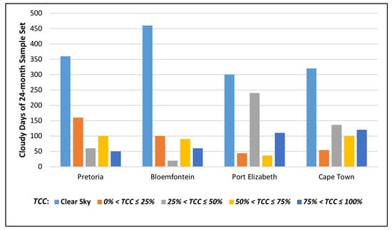
Figure 2.
Summary of the cloud conditions for the four locations.

Table 1.
Standard Deviation Error Comparison, Pretoria.
Table 2.
Standard Deviation Error Comparison, Bloemfontein.
Table 3.
Standard Deviation Error Comparison, Port Elizabeth.
Table 4.
Standard Deviation Error Comparison, Stellenbosch.
The average forecast error improvement across all sites is given in Figure 3. The figure contains values based on the average difference between the GHI and the GMOS forecast for the full forecast horizon, including the condition of the TCC.
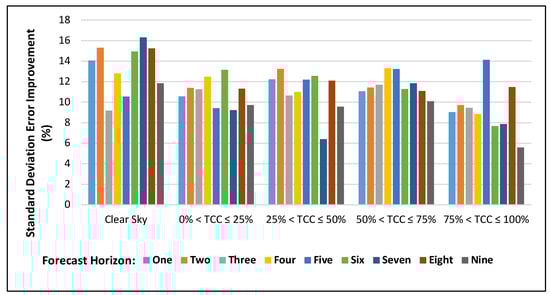
Figure 3.
These values depict the average difference between the Meteomatics AG Global Horizontal Irradiance (GHI) and the Gridded Model Output Statistics (GMOS) GHI forecast errors for all four cites combined concerning the conditions of the Total Cloud Cover (TCC) and the forecast horizon.
From Figure 3, it is evident that significant forecast improvements have been achieved with clear sky conditions, decreasing performance as the sky is covered with more clouds. An overall average improvement of 11.28% is seen regarding all cloud conditions across the entire time horizon. It is, however, interesting to note the somewhat out of trend error improvement of the 50% < TCC ≤ 75%, which may require further investigation in future work. Table 5 contains the average forecast performance for the four locations combined.
Table 5.
Standard Deviation Error, Average Across All Aites.
Throughout Table 1, Table 2, Table 3 and Table 4, it is noticeable that the forecast accuracy deteriorates gradually with an increase in TCC. This is mainly due to the increasing difficulty of forecasting GHI accurately with the accumulation of clouds [21]. No significant error trend was found with this data when observing the forecast horizon. On average, the coastal city of Port Elizabeth (Table 3) is seen to have the best clear sky and 0% < TCC ≤ 25% GHI forecast performance.
The variation in GHI forecast accuracy is most likely due to site-specific forecast model characteristics from the source, the amount of site-specific historical data available to the source forecast model when it was created or trained and the level of the Air Quality Index (AQI) at any specific location. The AQI is a function of the amount of carbon monoxide (CO), sulfur dioxide (SO2), nitrogen dioxide (NO2), fine particulate matter (PM2.5), respirable particulate matter (PM10), and ozone (O3) in the air [22]. It has been shown that the AQI level is a strong contributor to the GHI forecast accuracy of a specific location subjected to air pollution or haze [22,23,24,25]. The South African Air Quality Information Systems (SAAQIS) [26], in Pretoria South Africa, provided the following annual average AQI values of the four locations which include their immediate surroundings: Pretoria (92), Bloemfontein (32), Port Elizabeth (16), and Stellenbosch (44). A useful graphical representation of the AQI levels of South Africa can be seen here [27].
Although convective weather conditions (formation of clouds) generally decrease the GHI forecast accuracy (as seen in Table 1, Table 2, Table 3 and Table 4), the GHI forecast model prediction will also be affected by the AQI. The effect of the AQI on the GHI forecast skill is most prominent during clear sky and near clear sky conditions. Port Elizabeth displays the lowest average AQI of the four locations under investigation. The first two columns of Table 3 (clear sky and 0% < TCC ≤ 25%) displays the best GHI forecast skill when compared to the other locations. The remaining three columns (25% < TCC ≤ 100%) of Table 3 more closely resembles that of the other three locations showing that the AQI has a less significant effect in the presence of substantial clouds. This is probably due to the fact that the presence of cloud will decrease the forecast accuracy by larger magnitudes and with the mixture of clouds and high AQI levels, the effect on the accuracy is combined and a distinction between the effect of the one and the other becomes hard to establish.
The mean forecast performance std error of the Meteomatics AG GHI and GMOS GHI model for the combination of the four sites across the whole forecast horizon is shown in Table 6 (corresponding RMSE values are in brackets):
Table 6.
Mean forecast performance summary
These mean forecast performance std values subsequently confirm the expected increasing error trend with the increase in cloud cover [21]. An overall (all clouds conditions and full forecast horizon over all four locations) mean forecast performance std improvement of 11.28% is observed after the GMOS correction model has been applied to the raw Meteomatics AG API data. It is noteworthy that the large observation set used, and relative low bias characteristics of the Meteomatics AG forecast [28] yielded the std error and RMSE values nearly identical [29].
4. Discussion
4.1. Energy Forecasting for a Solar Car in South Africa
The solar car team from Tshwane University of Technology (TUT) participated in the SSC 2018 with a solar car named Sun Chaser III (SCIII). The team had developed an energy simulation platform to assist the energy manager in making informed decisions in regards to the speed and distance they should travel each day based on the dynamics of the car, the route to be driven, the weather conditions, and other characteristics such as remaining stored battery energy. The authors [30] showed simulated SoC results compared to real-life recorded data during the SSC 2018 for SCIII for five of the eight days. The remaining three days’ data was not recorded due to technical difficulties.
Figure 4 shows the SCIII solar car followed by its telemetry support vehicle responsible for recording and analyzing data during the SSC 2018 [30].
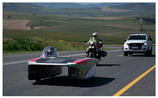
Figure 4.
Sun Chaser III (SCIII) and its telemetry support vehicle during the SSC 2018 event.
In 2018, these SoC simulations did not make use of the GMOS model described in this work. Figure 5, Figure 6 and Figure 7 show how the GMOS model could have improved the GHI forecast accuracy for the same data as the authors used in [30] and how this relates to an improvement in the accuracy of the predicted SoC for SCIII during the SSC 2018. The authors referred to three specific days during the SSC 2018: day one, six, and eight. During these days, the elements (weather parameters and driving speed) negatively impacting on the SoC accuracy were minimal. This resulted in the GHI forecast accuracy to be one of the most significant contributors to the remaining SoC errors observed on these days. Table 7 provides a summary of all five days during the SSC 2018 recorded by the TUT team and SCIII [30].
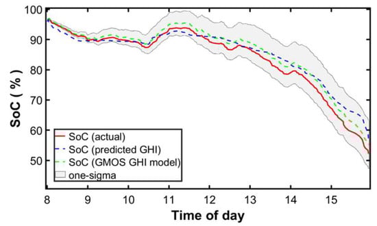
Figure 5.
SSC 2018 day one.
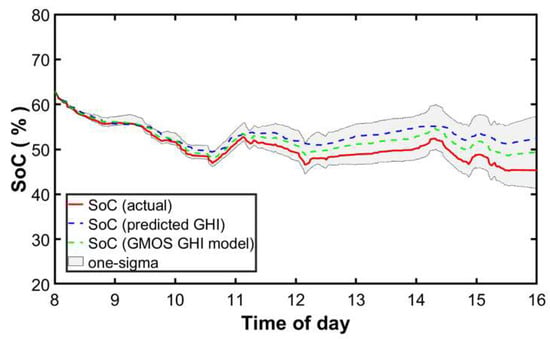
Figure 6.
SSC 2018 day six.
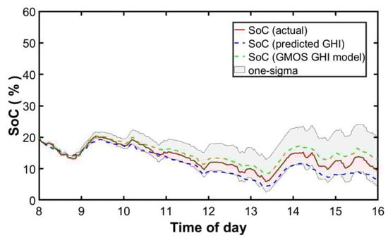
Figure 7.
SSC 2018 day eight.
Table 7.
Sun Chaser III results during the SSC 2018.
The red and blue plots are the real-life recorded and simulated SoC behaviors during the SSC 2018 for the SCIII solar car [30]. The green plot is the improved GMOS GHI model simulation of this work. Furthermore, these figures contain the GMOS GHI std (one-sigma) upper and lower bounds (confidence intervals) based on a continuation of the most extreme expected GMOS GHI std error in the forecast. SoC forecast improvements are observed on all three days; the first and sixth days, the GMOS GHI model followed suit and still over predicted, however, with fewer errors than the original predictions. On the last day (Figure 7, day eight), the original model under-predicted where the GMOS model yet again over-predicted, however, still with less absolute error.
Figures for the remaining two days of the SSC 2018 with valid data, day four and day seven, are shown in Figure 8 and Figure 9. They were intentionally grouped separately from day one, six, and eight. The inaccuracy of the simulations of these days is attributed to the significant deviation from the simulation speed profile [30] during the SSC 2018. These two days highlight the effect that a gross deviation from the speed profile of the simulation has on the accuracy of the SoC. In fact, the speed deviation had such a devastating impact on the accuracy of the SoC results that the GMOS GHI improvement is insignificant on days four and seven.
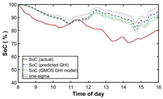
Figure 8.
SSC 2018 day four.
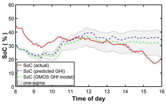
Figure 9.
SSC 2018 day seven.
The amount of speed deviation (RMSE of the simulated speed compared to the actual speed) that brought about these significant errors on day four and day seven is 41.67% and 62.32%, respectively. In contrast, the speed RMSE values for day one, six, and eight have a minimum of 14.46% on day six and a maximum of 16.56% on day eight [30]. Hence, the GMOS GHI model has a much more significant impact on the outcome of the SoC simulation accuracies for these three days.
Table 8 shows the GMOS performance results for the five days of the Sasol Solar Challenge 2018. It contains the actual, initially predicted, as well as GMOS compensated SoC final values. Also, the RMSE values for the SoC are also shown here.
Table 8.
GMOS Performance Results.
The GMOS GHI model performance results for day four and seven is of no real value when characterizing the overall performance of the applied method. Hence, the performance details of these two days will be omitted in the following sections.
Considering days one, six, and eight: the mean SoC RMSE of the initially predicted GHI forecast is 1.55%, in contrast with the improved 1.10% RMSE of the GMOS GHI. Considering the final SoC of each day, the GMOS GHI model had the most substantial impact on day six (4% SoC closer to the actual SoC) and the smallest impact (1% SoC closer to the actual SoC) on day eight. The reason for this is that day six had the lowest wind and other weather variable errors [30] leaving the GHI accuracy to have a significant impact on the SoC. Day eight, however, experienced significant wind forecast errors (nearly double of day six) which resulted in the effect of the improved GHI accuracy to be less on the SoC for that day.
In addition to the SoC improvements, the energy simulation user can now also visualize the amount of statistical risk involved in a simulation which will aid in critical decision making regarding the energy expenditure of the vehicle during a Sasol Solar Challenge or similar event.
4.2. GMOS Benefits to a Solar Car Team
An energy manager of a solar car team would not drain the Li-Ion battery to less than 1% of capacity. Even with a 1% overall capacity remaining, it is not uncommon to see the individual cells which make up the battery pack differ marginally in charge voltage (unbalanced battery). If a cell operates below its absolute minimum or maximum voltage rating, the cells might be severely and permanently damaged. Furthermore, the cells’ chemical behavior becomes unstable beyond the absolute ratings, which might result in a fire hazard [31].
On the last day of the SSC 2018, the envisaged final SoC for SCIII was 6.18% (Table 8 and Figure 7), which was acceptable to the energy manager as it was above 1%. The energy manager did at that time not have any access to quantify simulation risk, and therefore, a 5% margin above the prediction seemed acceptable at the time (based on intuition).
If the energy manager at that time had access to the more accurate less biased GMOS GHI forecast, they would have realized that traveling 403 km for the day (Table 7) might leave their battery underutilized at 13.31% SoC (Table 8 and Figure 7) at the end of the day. Currently, the lower and upper bound of the confidence interval is approximately 8% above and 8% below the green GMOS GHI prediction plot by 16:00. To keep within the interval, the energy manager might aim to drain the battery to 9%, which ensures the lower confidence bound is at 1% in a worst-case situation. This means that the car theoretically now has access to 1.1% more SoC energy (assuming the GMOS GHI forecast is absolutely accurate) to expend while taking minimal risk in doing so. The theoretical 1.1% was calculated by the difference between actual final SoC recorded and the expected final GMOS GHI prediction if the lower bound was at 1%.
The total SoC expended to cover 403 km was 9.97% (calculated from Table 8). The average energy economy (ratio of SoC energy to distance) of SCIII on day eight of the SSC 2018 was 0.0247% SoC per kilometer. One has to keep in mind that this average energy economy is based on the average speed driven for that specific day. If more distance needs to be covered on the same day and during the same time, the average speed will need to be increased. In turn, the aerodynamic forces increase with a quadratic function [32,33] with speed, and hence, the average energy economy will be different at higher speeds.
Furthermore, it is imperative to understand that more accurate forecasts do not directly constitute further distance traveled. The energy manager’s interpretation of an SoC simulation, as well as the amount of error in the forecast and the driving speed, determines the actual distance traveled and remaining SoC at the end of a day. The improved GMOS GHI accuracy simply reduces some of the error and risk involved when an energy manager interprets an SoC plot in order to guide a solar car team towards the most energy-conscious movements of the solar car.
Considering a constant energy economy of 0.0247% SoC per kilometer, and having taken into account the limitations of this value and others mentioned, access to the theoretical 1.1% excess SoC might have increased the distance of SCIII an average of 44.4 km on the last day of the SSC 2018.
4.3. MOS vs. GMOS Performance
It is essential to evaluate the effectiveness of the interpolation between the MOS models (Equation (1) for all four locations), which gave birth to the GMOS model (Equation (2)). Each of the three useful days (day one, six, and eight) were re-simulated with a MOS model of the nearest ground observation station to its rear, as well as with a MOS model of the nearest ground observation station to the front of the car. This is done to quantify the performance effect it would have on the SoC in comparison with the interpolated GMOS model. Table 9 contains the comparative results.
Table 9.
GMOS vs. MOS Performance Results.
The GMOS model is a function of linear interpolation between two ground measurement locations (two MOS models) based on the current location. The corresponding two MOS models are, however, conditional statistical models based on the cloud conditions as well as the forecast horizon, and most importantly, the time of day. Therefore, it is not trivial to expect a visible linear relationship in the performance results of the rear and front MOS models compared to their corresponding GMOS model. Throughout Table 9, it is evident that the GMOS GHI model does produce improved forecast performance. There is one exclusion, on day eight, where the front location MOS model outperformed the GMOS model by 0.42% SoC error. On every other account, the GMOS model outperformed the individual MOS models.
4.4. Further Research Recommendations
This work is currently only focused on improving the GHI forecast component; however, the wind velocity and air density forecast performance can benefit from a similar method of improvement. By conditioning these additional environmental variables, the SoC error results will improve even further, ensuring sharper and more robust estimations for the energy manager and solar car team to benefit from. Finally, the use of a higher resolution grid (increasing the number of ground measurement locations) to create the GMOS GHI model will further enhance the results.
5. Conclusions
The improvement to the local (South African) GHI forecast has had a significant positive impact on the SoC energy simulations of the SCIII solar car during the SSC 2018. The gridded-MOS model was shown to be practical and useful. The GMOS model has shown forecast improvements for all sky conditions in South Africa, and the AQI was also found to have an impact on location based GHI forecasts. Events such as the Sasol Solar Challenge take place over eight days and typically span more than 2000 km. Having access to more accurate SoC simulations over these eight days could provide the team with an advantage. This will enable them to make more informed energy decisions which could result in critical choices such as including additional route sections (increasing distance traveled), putting them ahead of their nearest rivals. A secondary outcome of this work is that the SoC energy simulation now has some statistical confidence intervals which are extremely valuable especially in situations where simulation risk needs to be quantified for inclusion in the decision-making process by the team energy manager.
Author Contributions
Conceptualization, C.O. and B.V.W.; methodology, B.V.W. and C.O.; software, C.O.; validation, D.D., Y.A., and Y.H.; formal analysis, C.O.; investigation, C.O.; resources, Y.A. and B.V.W.; data curation, C.O.; writing—original draft preparation, C.O.; writing—review and editing, D.D., B.V.W., Y.H., and Y.A.; visualization, C.O.; supervision, B.V.W. and Y.H.; project administration, C.O.; funding acquisition, B.V.W., Y.A., and C.O. All authors have read and agreed to the published version of the manuscript.
Funding
This research as well as the APC was funded by the “Tshwane University of Technology (TUT) & the manufacturing, engineering and related services Sector Education and Training Authority (merSETA) Chair in Intelligent Manufacturing”. The forecast weather data used in this research was sponsored by “Meteomatics AG”.
Acknowledgments
The authors would like to thank Meteomatics AG for the sponsorship of the forecast data and the merSETA and TUT chair in Intelligent Manufacturing for their financial assistance.
Conflicts of Interest
The authors declare no conflict of interest.
References
- Porter, J. Toyota Is Testing a Much More Efficient Solar Roof for Its Electric Cars. 2019. Available online: https://www.theverge.com/2019/7/5/20683111/toyota-prius-plug-in-hybrid-solar-roof-range-electricity-energy-environment (accessed on 5 February 2020).
- Harrop, P. IDTechEx Explains Significance of Driving Tesla and Squad Solar. 2019. Available online: https://www.idtechex.com/en/research-article/idtechex-explains-significance-of-driving-tesla-and-squad-solar/18881 (accessed on 2 February 2020).
- Lightyear. Lightyear One Designed for performance. 2020. Available online: https://lightyear.one/lightyear-one/ (accessed on 6 January 2020).
- Mambou, E.N.; Swart, T.G.; Ndjiounge, A.R.; Clarke, W.A. Design and implementation of a real-time tracking and telemetry system for a solar car. In Proceedings of the AFRICON 2015, Addis Ababa, Ethiopia, 14–17 September 2015. [Google Scholar]
- Oosthuizen, C.; Wyk, B.V.; Hamam, Y. Modelling and simulation of the South African designed Sun Chaser II solar vehicle. In Proceedings of the 2017 IEEE AFRICON, Cape Town, South Africa, 18–20 September 2017. [Google Scholar]
- Lu, H.; Zhang, Y.; Cai, J. Consistency and differences between remotely sensed and surface observed total cloud cover over China. Int. J. Remote Sens. 2015, 36, 4160–4176. [Google Scholar] [CrossRef]
- Chan, K.L.; Wiegner, M.; Flentje, H.; Mattis, I.; Wagner, F.; Gasteiger, J.; Geiß, A. Evaluation of ECMWF-IFS (version 41R1) operational model forecasts of aerosol transport by using ceilometer network measurements. Geosci. Model Dev. 2018, 11, 3807–3831. [Google Scholar] [CrossRef]
- White, G.; Yang, F.; Tallapragda, V. The Development and Success of NCEP’s Global Forecast System; National Oceanic and Atmospheric Administration: Silver Spring, MD, USA, 2018.
- Radar, V. Top Meteorology Companies. 2019. Available online: https://www.ventureradar.com/keyword/Meteorology (accessed on 4 September 2019).
- Agüera-Pérez, A.; Palomares-Salas, J.C.; de la Rosa, J.J.G.; Florencias-Oliveros, O. Weather forecasts for microgrid energy management: Review, discussion and recommendations. Appl. Energy 2018, 228, 265–278. [Google Scholar] [CrossRef]
- Nespoli, A.; Ogliari, E.; Leva, S.; Pavan, A.M.; Mellit, A.; Lughi, V.; Dolara, A. Day-Ahead Photovoltaic Forecasting: A Comparison of the Most Effective Techniques. Energies 2019, 12, 1621. [Google Scholar] [CrossRef]
- Ruth, D.P.; Glahn, B.; Dagostaro, V.; Gilbert, K. The Performance of MOS in the Digital Age. Weather Forecast. 2009, 24, 504–519. [Google Scholar] [CrossRef]
- Shin, Y.; Yi, C. Statistical Downscaling of Urban-scale Air Temperatures Using an Analog Model Output Statistics Technique. Atmosphere 2019, 10, 427. [Google Scholar] [CrossRef]
- Bofinger, S.; Heilscher, G. Solar electricity forecast: Approaches and first results. In Proceedings of the 21st European Photovoltaic Solar Energy Conference and Exhibition, Dresden, Germany, 4–8 September 2006. [Google Scholar]
- Lorenz, E.; Hurka, J.; Heinemann, D.; Beyer, H.G. Irradiance Forecasting for the Power Prediction of Grid-Connected Photovoltaic Systems. IEEE J. Sel. Top. Appl. Earth Obs. Remote Sens. 2009, 2, 2–10. [Google Scholar] [CrossRef]
- Diagne, M.; David, M.; Boland, J.; Schmutz, N.; Lauret, P. Post-processing of Solar Irradiance Forecasts from WRF Model at Reunion Island. Energy Procedia 2014, 57, 1364–1373. [Google Scholar] [CrossRef]
- Verzijlbergh, R.A.; Heijnen, P.W.; de Roode, S.R.; Los, A.; Jonker, H.J.J. Improved model output statistics of numerical weather prediction based irradiance forecasts for solar power applications. Solar Energy 2015, 118, 634–645. [Google Scholar] [CrossRef]
- Troccoli, A.; Morcrette, J.-J. Skill of Direct Solar Radiation Predicted by the ECMWF Global Atmospheric Model over Australia. J. Appl. Meteorol. Climatol. 2014, 53, 2571–2588. [Google Scholar] [CrossRef]
- Perez, R.; Lorenz, E.; Pelland, S.; Beauharnois, M.; van Knowe, G.; Hemker, K.; Heinemann, D.; Remund, J.; Müller, S.C.; Traunmüller, W.; et al. Comparison of numerical weather prediction solar irradiance forecasts in the US, Canada and Europe. Solar Energy 2013, 94, 305–326. [Google Scholar] [CrossRef]
- Brooks, J.B.; Clou, S.d.; van Niekerk, W.; Gauche, P.; Leonard, C.; Mouzouris, M.J.; Meyer, R.; van der Westhuizen, N.; van Dyk, E.E.; Vorster, F.J. SAURAN: A new resource for solar radiometric data in Southern Africa. J. Energy South. Afr. 2015, 26. [Google Scholar] [CrossRef]
- Kosmopoulos, P.G.; Kazadzis, S.; Lagouvardos, K.; Kotroni, V.; Bais, A. Solar energy prediction and verification using operational model forecasts and ground-based solar measurements. Energy 2015, 93, 1918–1930. [Google Scholar] [CrossRef]
- Fan, J.; Wu, L.; Zhang, F.; Cai, H.; Wang, X.; Lu, X.; Xiang, Y. Evaluating the effect of air pollution on global and diffuse solar radiation prediction using support vector machine modeling based on sunshine duration and air temperature. Renew. Sustain. Energy Rev. 2018, 94, 732–747. [Google Scholar] [CrossRef]
- Ehteram, M.; Najah, A.-M.; Chow, M.F.; Afan, H.; El-Shafie, A. Accuracy Enhancement for Zone Mapping of a Solar Radiation Forecasting Based Multi-Objective Model for Better Management of the Generation of Renewable Energy. Energies 2019, 12, 2730. [Google Scholar] [CrossRef]
- Peters, I.M.; Karthik, S.; Haohui, L.; Buonassisi, T.; Nobre, A. Urban Haze and Photovoltaics. Energy Environ. Sci. 2018, 11, 3043–3054. [Google Scholar] [CrossRef]
- Suthar, M.; Singh, G.K.; Saini, R.P. Effects of air pollution for estimating global solar radiation in India. Int. J. Sustain. Energy 2017, 36, 20–27. [Google Scholar] [CrossRef]
- Gwaze, P.; Mashele, S.H. South African Air Quality Information System (SAAQIS) mobile application tool: Bringing real time state of air quality to South Africans. Clean Air J. 2018, 28, 3. [Google Scholar] [CrossRef]
- Labs, P. World Air Map. 2020. Available online: https://air.plumelabs.com/en/ (accessed on 4 April 2020).
- Gericke, G.A.; Luwes, N.; Mqaqa, V.S. Solar Irradiance Model for the South African Solar Challenge. In 2019 Southern African Universities Power Engineering Conference/Robotics and Mechatronics/Pattern Recognition Association of South Africa (SAUPEC/RobMech/PRASA); IEEE: Piscataway, NJ, USA, 2019. [Google Scholar]
- Meyer, T. Root Mean Square Error Compared to, and Contrasted with, Standard Deviation. Surv. Land Inf. Sci. 2012, 72, 107–108. [Google Scholar]
- Oosthuizen, C.; van Wyk, B.; Hamam, Y.; Desai, D.; Alayli, Y.; Lot, R. Solar Electric Vehicle Energy Optimization for the Sasol Solar Challenge 2018. IEEE Access 2019, 7, 175143–175158. [Google Scholar] [CrossRef]
- Stephens, D.; Shawcross, P.; Stout, G.; Sullivan, E.; Saunders, J.; Risser, S.; Sayre, J. Lithium-Ion Battery Safety Issues for Electric and Plug-in Hybrid Vehicles; National Highway Traffic Safety Administration: Washington, DC, USA, 2017.
- Kwon, H. A study on the resistance force and the aerodynamic drag of Korean high-speed trains. Veh. Syst. Dyn. 2018, 56, 1250–1268. [Google Scholar] [CrossRef]
- Libii, J.N. The determination of the aerodynamic drag force on a parachute. World Trans. Eng. Technol. Educ. 2007, 6, 97. [Google Scholar]


© 2020 by the authors. Licensee MDPI, Basel, Switzerland. This article is an open access article distributed under the terms and conditions of the Creative Commons Attribution (CC BY) license (http://creativecommons.org/licenses/by/4.0/).