Abstract
In the smart grid environment, the penetration of electric vehicle (EV) is increasing, and dynamic pricing and vehicle-to-grid technologies are being introduced. Consequently, automatic charging and discharging scheduling responding to electricity prices that change over time is required to reduce the charging cost of EVs, while increasing the grid reliability by moving charging loads from on-peak to off-peak periods. Hence, this study proposes a deep reinforcement learning-based, real-time EV charging and discharging algorithm. The proposed method utilizes kernel density estimation, particularly the nonparametric density function estimation method, to model the usage pattern of a specific charger at a specific location. Subsequently, the estimated density function is used to sample variables related to charger usage pattern so that the variables can be cast in the training process of a reinforcement learning agent. This ensures that the agent optimally learns the characteristics of the target charger. We analyzed the effectiveness of the proposed algorithm from two perspectives, i.e., charging cost and load shifting effect. Simulation results show that the proposed method outperforms the benchmarks that simply model usage pattern through general assumptions in terms of charging cost and load shifting effect. This means that when a reinforcement learning-based charging/discharging algorithm is deployed in a specific location, it is better to use data-driven approach to reflect the characteristics of the location, so that the charging cost reduction and the effect of load flattening are obtained.
1. Introduction
As environmental problems, such as climate change caused by global warming and air pollution, have become global issues, electric vehicle (EV) are considered as an alternative to vehicles that use fossil fuels. Accordingly, the distribution of EVs and charging stations is increasing rapidly with government investments [1]. This increasing number of alternative vehicles will change the existing load profile, and it may affect the grid in terms of power loss and voltage deviation. Therefore, coordination for EV charging is crucial [2].
Additionally, as the proportion of renewable energy generation increases, a method is required to control the intermittence and volatility of its generation and to increase the reliability of the smart grid. Among the several available methods, a demand-side management mechanism using dynamic pricing is broadly utilized to shift load from on-peak to off-peak periods [3]. There are several types of dynamic pricing schemes. For example, the most common one is time-of-use (ToU) [4], under which electricity price varies depending on whether the current time zone is on-peak or off-peak. Another scheme is the hourly pricing scheme, usually called real-time pricing [5]. In this scheme, the electricity price changes every hour. A power company, “ComEd” in Illinois, USA, has introduced the hourly pricing scheme for EVs and residential customers. Electricity pricing schemes are developing towards real-time pricing, which is more economically efficient as it directly reflects supply and demand. Meanwhile, vehicle-to-grid (V2G) technology [6] is being introduced, and EV batteries are also gaining recognition as an energy resource by supplying energy to the grid [7]. Therefore, considering that dynamic pricing and V2G are being introduced, it would be beneficial to schedule real-time charging/discharging in response to the price signal, as this makes it possible to minimize EV charging costs and ensure grid reliability [8]. However, this would be difficult to achieve as, practically, an EV user cannot control charging/discharging by monitoring the price signal in real-time. Hence, it is imperative to develop an algorithm that automatically conducts the decision making of charge/discharge in response to the price signal.
Several papers studying EV scheduling problem with various optimization methods have been published. The optimization methods that can be applied to EV charging/discharging scheduling problem can be divided into two categories. In the first case, EV charging/discharging scheduling problem is usually considered as a sequential decision-making problem, which is modeled as the Markov decision process (MDP) [9,10,11,12,13,14] and then solved by dynamic programming [15]. The second case involves the use of conventional numerical optimization methods, such as linear programming or convex optimization [16,17,18,19,20,21,22,23,24]. However, these optimization-based methods have their drawbacks: they require mathematical model with some assumptions that are hardly known in practice. In particular, conventional numerical optimization methods mostly aim at planning for given scenarios, which is usually often predicted using a forecasting model. However, the result of the optimization highly depends on the accuracy of the forecasting model. In addition, in the case of dynamic programming-based methods, they require a model that mathematically represents transition in states that occurs when an agent takes an action, which is generally not known in real world.
Model-free reinforcement learning (RL) approaches have recently attracted attention for their human-like performances in complex decision-making problems [25]. The advantage of model-free RL over the optimization-based methods is that they do not rely on prior knowledge of an exact model information and learn the best actions through repeated trial and error. There have been studies that apply RL to the EV charging and discharging problems. Wan et al. [26] proposed a model-free deep RL (DRL) algorithm for charging/discharging scheduling of domestic EV. After obtaining a feature vector containing a future price trend using long short-term memory (LSTM) network from the historical price data, the MDP state is composed together with the current state of charge (SOC) amount. Then, an agent that conducts optimal decision-making of charging/discharging is generated by utilizing the deep Q-network (DQN) algorithm. The user-driving pattern, i.e., arrival and departure times and SOC at arrival, is assumed to follow the truncated normal distribution with mean and variance, roughly estimated based on commuting patterns of ordinary people. This study showed that charging costs can be minimized by scheduling the charging/discharging of EVs using RL in stochastic and complex situations. Their simulation results also present that it is better to use RL than to use an optimization algorithm with forecasting model. Shi et al. [27] proposed a real-time V2G control algorithm to decide whether the EV should be charged, discharged, or provided frequency regulation. They modeled the hourly-determined price using the Markov chain, and then Q-learning was used to learn control operation to maximize profit for the EV’s owner during parking time. They assumed that the EV arrives at 6:00 p.m. in the afternoon with an SOC of 40% every day and departs at 8:00 a.m. the following morning with an expected departure SOC of 70%. Dimitrove et al. [28] also proposed RL-based charging algorithms to maximize the profits of specific EV charging stations with renewable sources. Considering electricity price and the amount of renewable energy generated hourly, the amount of charge of the dynamically arriving EVs is determined using the learned Q-learning agent. In this study, vehicle arrivals were modeled using a non-homogeneous Poisson process and the number of cars arriving at time intervals was estimated from the data. Vandael et al. [29] focused on deciding a day-ahead consumption plan for charging a fleet of EVs. To address the complexity of various factors, they used the heuristic control scheme and subsequently, used the resulting behavior as the learning resource for the RL agent. Here, their reference scenarios were formed from assumptions about the arrival time, departure time, and requested charging amount. Chis et al. [30] modeled a plug-in electric vehicle (PEV) battery-charging problem as MDP with unknown transition probabilities. Then, they proposed a state–action–reward–state–action (SARSA) with eligibility traces for learning the price patterns and for solving the charging problem. They used known day-ahead prices and predicted prices for the second day-ahead. They also assumed to know daily driving patterns of the car’s user [31], formulated the EV charging and discharging scheduling problem as a constrained Markov decision process (CMDP). With the purpose of minimizing the charging cost while making sure that the EV is fully charged, they proposed safe deep reinforcement learning (SDRL) to solve CMDP. They used one-year of real-world electricity price data and assumed that the EV user’s driving behavior, such as arrival/departure time and battery energy follows truncated normal distributions.
The previous paragraph reviewed previous studies on EV scheduling using RL especially focusing on how the user’s driving patterns such as arrival time, departure time, and SOC at arrival are set. These were set as fixed values or normal distribution based on the life patterns of ordinary people, or they were modeled as a stochastic process using the Poisson process. However, in this way the above methods are insufficient to reflect the usage pattern of a specific charger or the pattern of various users who uses the charger, which means they are not appropriate to directly deployed in a real site. For example, if an agent is trained only with fixed arrival and departure times, it will learn to respond correctly only during that period. Similarly, an agent trained with variables sampled from a normal distribution would be an algorithm that is only suitable for vehicles operating within that range. The driving pattern of users will differ for each charging station; thus, it must be trained to reflect, effectively, its characteristics for correct scheduling. Therefore, this study proposes a RL with data-driven approach for EV charging and discharging problem. This study aims to estimate the probability density functions from EV charging data using kernel density estimation (KDE). Scenarios sampled from the density function were used to train a DRL agent to reflect the usage pattern of a specific charger so that the algorithm can be effectively deployed realistically.
The contributions of this study are summarized as follows:
- 1.
- We developed a method to train a model-free RL agent that makes decisions on charging and discharging in a data-driven approach using nonparametric probability density estimation. The major advantage is that it can reflect the usage pattern of a specific charger at a specific location so that the agent can be trained to suit the characteristics of the target location. This will be helpful when deploying the algorithm to the actual site.
- 2.
- Unlike previous studies focusing on one charger per person, we considered the case where one public charger is used by several users, which means it trains a RL agent that can cover several charges a day. In other words, by utilized data-driven method for a specific charger in a specific location, this method can be applied to a public charger shared among multiple users.
The remaining part of this paper is organized as follows: Section 2 describes the scheduling problem and a system model in detail. Section 3 presents the RL algorithm that was used to solve the scheduling problem and also explains the data-driven probability density estimation method using KDE. In Section 4, the simulation results are presented to show the superiority of the proposed method. Finally, Section 5 gives the conclusion.
2. System Model
In this section, the real-time EV charging and discharging scheduling problem is formulated as MDP from a single charger’s point of view. The goal of scheduling is to smartly charge EVs to reduce charging costs for users while contributing to the system’s operation by responding to price signals. Hence, decisions should be made hourly on charging and discharging according to the current state. This study targets a single, specific public charger, thus multiple cars can visit each single day as shown in Figure 1. When a car is connected to a charger, the charging and discharging scheduling period is regarded as the period from the start of charging until the completion of charging and departure. When a car comes and starts charging, we seek an algorithm that automatically charges and discharges in response to the price signal and eventually charges fully.
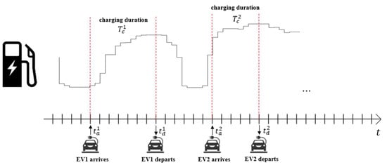
Figure 1.
A situation where multiple electric vehicles (EVs) arrive at a single charger in a specific location and charge during the charging period under hourly pricing scheme.
We formulate this problem with finite MDP with discrete time step. At every time step t, which is an hour in our case, the state that contains information such as historical price, current energy level in the EV battery, etc. is observed. A decision is selected by the algorithm to determine the charging and discharging rate from the vehicle’s arrival time to the departure time with duration , according to the past k-step price determined every hour. It is assumed that corresponds to charging start time, and also corresponds to the departure time of the EV after completion of charging. After every is taken, immediate reward and next state are observed, and the process is repeated. The reward and the next state are given from a system called “environment” as a RL term, and the entity that takes actions is called “agent”. A mathematical framework for modeling this decision-making is formulated using MDP, which is defined as 4-tuple , where each term corresponds to state, action, transition probability, and reward, respectively. The scheduling problem defined by this tuple can be expressed as follows:
- 1.
- State: state at time step is defined as where represents past -step of hourly electricity price, represents current energy level left in the EV’s battery, represents the amount of energy left until the battery is fully charged, and represents the time remaining until the charge is complete.
- 2.
- Action: an action refers to charging and discharging power. When is positive, the EV charges; otherwise, it discharges. This study assumes that the charging/discharging power can be set in several levels. For instance, action space can be defined as where is the charging/discharging power.
- 3.
- Transition probability: transition probability denoted as is the probability that action in state at time will lead to state at time . In this study, as we utilize model-free RL algorithm, which will be described in Section 4, it was assumed that the transition probability is unknown; hence, it was estimated through interaction with the environment.
- 4.
- Reward: reward is the immediate reward obtained after the state transitions from to due to action . The reward in this study is defined as
An interaction between an agent and an environment is shown in Figure 2, where , represent random variables that follow the probability distribution of , , and (an initial amount of energy left on an arrival of EV) derived by KDE, which will be discussed in Section 3.1.
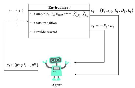
Figure 2.
An interaction between a reinforcement learning (RL) agent and an environment.
3. Proposed Method
In this section, we propose a method to solve the real-time EV charging/discharging scheduling problem under dynamic pricing that reflects the usage pattern of a specific charger in a specific location. We used the KDE to model the probability distribution of the usage pattern of a specific charger in a specific location. Then, the scheduling problem was solved using the DQN, which is a model-free RL algorithm. In the training process of the DRL agent, the variables related to the usage pattern sampled from the probability distribution made by KDE were cast.
3.1. Data-Driven Modeling of Charger Usage Patterns
KDE is a nonparametric method of estimating the probability distribution of an unknown random variable. In other words, KDE estimates the distribution of a population from a data sample and can also be considered as a method of smoothing the histogram. The method is to create a kernel function for the observed data values, add them together, and then divide the sum by the number of data points. The popular kernel functions are uniform, triangular, and Gaussian. In this method, the density function estimated based on KDE can be mathematically expressed as follows:
where is the probability density function estimated using KDE, is the data sampled from the probability distribution we want to know, is the number of samples, is a kernel function and is a smoothing parameter called bandwidth, and represents the thinness and thickness of the kernel function (the thinner it is, the more precisely it will fit into the observed data distribution, but it may not be generalized). Therefore, it is important to set to an appropriate value.
In this study, based on the charging data of the electric vehicle charger installed in the target location, the joint probability distribution for the tuple of arrival time and charging duration was generated using KDE as shown in Figure 3. Additionally, for simplicity, we assumed that the user always wants the battery to be fully charged, and the amount of energy remaining in the battery at the start of charging was estimated by considering the end time of charging and the efficiency of the charger. The estimated amount of energy was modeled as a probability distribution using KDE as well.
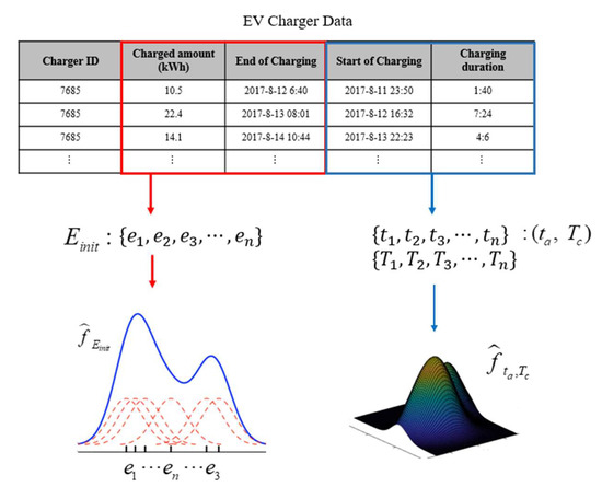
Figure 3.
Data-driven kernel density estimation (KDE) regarding initial energy in the battery when an EV arrives, and the tuple of EV arrival time and charging duration .
3.2. Solving Scheduling Problem using DRL
As mentioned in Section 3, the transition probabilities of MDP model are unknown. The only known thing about the hourly electricity price or the usage pattern of the target charger is their realization, not their true distribution. In other words, the model of the MDP is unknown, but the experience can be sampled. Model-free RL algorithm can be used in this situation as it can obtain optimal policies by continuously updating action-value functions. The action-value function numerically expresses how much reward is expected when taking action according to policy in any state . That is, it tells how good it is to take action in state , and it is expressed mathematically form as follows:
where is an action-value function when it follows policy , and is a value that determines the discount rate for future rewards. ranges between 0 and 1. The closer it is to 1, the future reward is converted to a value closer to the immediate value, and the closer it is to 0, the lower the value. The action-value function can be updated repeatedly using the Bellman equation, which is shown below.
By iteratively calculating this equation as approaches infinity, it converges to the optimal action-value function . The priority here is how to calculate the expected value . To perform iterative calculations, is required in the above equation. In other words, the model of the environment should be known. If the model of the environment is unknown, the action-value function should be updated iteratively with samples obtained from random actions. If the optimal action-value function is obtained, the Q-value of all possible actions in all states is known. Once the optimal action-value function is obtained, the value of every possible action in every state is known; thus, following the action with the highest Q-value becomes the optimal policy. The optimal policy is expressed mathematically as follows:
As the superiority has been demonstrated in previous studies [25,26], we approximate the action-value function as a neural network, which is the DQN. Using this, it is possible to use the price data without discretization, which is not possible in tabular form, and update the action-value function more efficiently. DQN also uses the experience memory and the target network. The samples obtained from the action are stored in the experience replay and then randomly sampled to train the Q-network. This way, the data usage efficiency can be improved by using data samples multiple times, and the high-correlation problem between successive states can be solved. Further, using the target network, we can solve the problem of non-stationary target when training the neural network. (Refer to [26] for a detailed description of DQN).
The process of developing the scheduling algorithm using the above method is the same as Algorithm 1. First, create an experience replay memory of size N and initialize the network parameters and of the Q-network and the target Q-network. Next, repeat M epochs and play K episodes per epoch. Episode here refers to one complete charging process. For each episode, and are sampled from the density functions and that were produced by the process discussed in Section 4.1. Afterward, the charging/discharging action is selected based on the ε-greedy algorithm for each time step of the episode. The ε-greedy algorithm refers to a policy that selects a random action with a probability of ε or selects an action based on an action-value function with a probability of 1-ε. This is to properly balance exploration and exploitation. ε is designed to decrease gradually as the epoch progresses. When an action is taken, the agent receives reward and next state . Then a tuple is stored in the replay memory as a sample. Further, a minibatch of #B samples is extracted from the experience replay memory to update the Q-network. Minibatch samples are used to calculate the target using Equation (6) below.
The error between the Q-value predicted by the action-value function and the calculated target for the sample is expressed as follows using mean squared error (MSE).
The gradient descent method is used to update the network parameter θ in minimizing the error function below, where refers to learning rate or step size and means gradient of the loss function.
Finally, at the end of each episode, copy the parameter of the target network to the parameter of the current local network. When the training of the agent is completed, Equation (5) can be used to select the charging/discharging action at every time step, thereby yielding the optimal scheduling results.
| Algorithm 1 Training of EV scheduling agent |
| 1: Initialize replay memory to capacity N. 2: Initialize action-value function with random weight . 3: Initialize target action-value function with weight . 4: For epoch = 1, M do 5: For episode = 1, K do 6: Get from and get from . 7: Get initial state from the environment 8: For do 9: Select charging/discharging action based on -greedy algorithm. 10: Execute action in environment and observe reward and next state . 11: Store transition sample in . 12: Sample random minibatch of transitions from . 13: Set 14: Calculate the loss function 15: Perform a gradient descent step on with respect to the parameter . 16: based on . 17: Reset . 18: End For 19: End For 20: End for |
4. Simulations Results and Discussions
In this section, we evaluate the effectiveness of the proposed method, i.e., DRL trained with charger usage patterns that were sampled from the probability distribution modeled by KDE. We first present the results of the KDE (Section 4.1) and then discuss the results of a charging/discharging scheduling performed by DRL agent (Section 4.2). Two residential (i.e., apartments) sites with EV chargers were tested: “Site A” and “Site B”. Simulation setup details are presented as well.
4.1. Modeling Charger Usage Patterns
To model the charger usage pattern using KDE, we used the EV charger data obtained from a charger at a specific location. The data contains information about charging amounts (kWh), charging duration, start time of charging, and end time of charging.
We assumed that EV owners want their vehicles to be charged fully as at when they depart. Although different types of EVs could be charged several times a day, for simplicity we also assumed that only Hyundai IONIQ with battery capacity 28 kWh arrives. Using this battery capacity, the charging duration given in the data, and 7 kW typical charging efficiency of a slow charger, the initial energy in a battery when EVs start charging was calculated. To conclude, the start time of charging and the charging duration were both used to model , and the calculated initial energy was used to model .
In Figure 4, Figure 5 and Figure 6, the results of the KDE on the start time of charging, charging duration, and initial energy for Sites A and B are shown. It can be observed that the shapes of density functions in Figure 4 and Figure 5 are far from the normal distribution. This means that as was done in the previous studies [26,28,31], if we had modeled the charger usage pattern variables as general probability distributions, such as normal distribution rather than KDE, we would be unable to properly reflect the characteristics of the target location. Further, from Figure 4 and Figure 5, it is evident that the distributions of samples from the estimated density functions are almost the same as the distributions of the actual data, which means the density functions were well estimated. Moreover, it is observed from Figure 4 that the distributions of the start time of charging in Sites A and B are nearly similar, but the charging duration of Site B tends to be shorter. Additionally, from Figure 5, it is evident that Site A tends to possess more battery energy than Site B when EVs arrive. In other words, the EVs arriving at Site A have much more room to discharge during the charging duration so that they can expect more benefits. By sampling the start time of charging, charging duration, and initial energy from density functions in Figure 6, and using them in a training process of a DRL agent, we can develop a scheduling algorithm that is optimized for the charger usage pattern at a specific location.
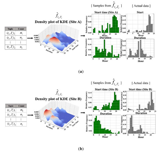
Figure 4.
Results of the kernel density estimation (KDE) for probability distributions of tuples of start time of charging and charging duration: (a) Site A; (b) Site B.
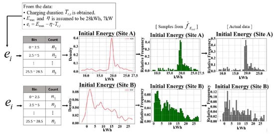
Figure 5.
Results of KDE for probability distributions of an initial energy at arrival of an EV for Sites A and B.
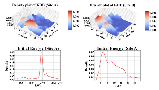
Figure 6.
Estimated density functions and using KDE for Site A and B.
4.2. Results of Solving Scheduling Problem Using DRL
In this section, the results of solving the scheduling problem are presented. In Section 4.2.1, the training process and the parameter settings are discussed. Then, in Section 4.2.2, benchmarks to compare with the proposed method are explained. The results of the scheduling of benchmarks and the proposed method are presented in Section 4.2.3. Finally, the effect of EV scheduling on a load profile of the target location is analyzed in Section 4.2.4.
4.2.1. Parameter Settings and Training Process of DRL
To train a DRL agent using real-world electricity price data, we used hourly electricity price data of the 31 days in August 2018 downloaded from Korea Power Exchange. Twenty-four days were used as the training set and the remaining as the test set. Strictly, this data is not the retail price data. However, as ComEd stated, the hourly retail price of electricity is determined by a wholesale price with almost the same trend. As the priority is to ascertain whether the agent can choose the charging/discharging action correctly for the fluctuating price, the available data will be applicable to the retail price data. We assumed that the charger provides several levels of charging/discharging rate (−4 kW, −2 kW, 0 kW, 2 kW, 4 kW), which directly corresponds to the action space. We set the discount factor to 0.99 to allow the agent to choose the current behavior considering future rewards. The neural network has two hidden layers and input/output layers. The number of units in the hidden layers was 32, and the number of units in the input layer is 14, which corresponds to the length of the state. The number of units in the output layer was understandably the same as the number of possible actions. The batch size was set to 128, and the learning rate for the neural network was set to 0.001. We allowed the agent to take random actions during the first 1250 epochs, which is equivalent to 5% of the total epochs of 25,000. Afterward, based on -greedy algorithm, the agent took an action depending on the Q-value predicted by the Q-network with probability , otherwise it took a random action. The value of was initially set to 1 during the random action period, which means the agent totally acted randomly in this period. After 1250 epochs, decays in the rate of 0.999 per epoch, which means that the agent is less likely to choose random action as the training progresses.
In Figure 7, the training process of a DRL agent is shown. As mentioned earlier, the agent acts randomly during the first 5% of the total number of epochs. Thus, until epoch 1250, the cumulative reward moves near −800,000 and then rises to around −100,000 because the agent acts based on -greedy algorithm, where gradually decreases. When remains at a minimum value, the training curve converges.
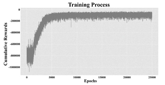
Figure 7.
Training process of the deep Q-network (DQN).
The training process takes about 8 h on the desktop computer equipped with i7-7700 CPU, NVIDIA GeForce GTX 1070 TI, and 16 GB RAM. The simulation program was developed with Python and Keras framework. After the training process finishes, a single schedule can be produced in about 5.2 ms.
4.2.2. Benchmarks
In this section, we introduce several benchmarks for comparisons to show the superiority of our proposed method. Our proposed method aimed to model the usage pattern of a specific charger in a specific location as a probability distribution. The variables sampled from this probability distribution in the DRL agent to reflect, effectively, the local characteristics. Therefore, it is required to compare the scheduling performance when the charger usage pattern is modeled by the existing methods that were used in the previous studies and by the proposed method. The existing methods are listed as follows:
- 1.
- Unscheduled (V0G): This is currently the most common charging method that charges directly from the moment the EV is connected to the charger. Sending electricity to the grid or responding to the price signal are not considered.
- 2.
- Charger usage pattern variables as fix values: In previous studies charging start time, charging duration, and initial energy were assumed as fixed variables in a common case (e.g., EV arrives at 7:00 p.m. and depart at 8:00 a.m., which is a general commuting pattern of most people) [27,29,30]. In this present study, instead of making assumptions in the general case, we averaged each value based on the charging data of a specific charger at a specific location and used that value as a fixed variable. For convenience, this method will be referred to as ‘FIX-RL’.
- 3.
- Charger usage pattern variables as random variables follow normal distribution: In a previous study, charging start time, charging duration, and initial energy were assumed to be random variables that follow the truncated normal distribution with mean and standard deviation assumed as the general case [26,31]. In our case, instead of making assumptions in the ordinary case, the mean and standard deviation of the normal distribution were derived from those of the data for corresponding variables. For convenience, this method will be referred to as ‘RV-RL’.
4.2.3. Scheduling Results
In this section, we evaluate the performance of the proposed method by comparing the scheduling results with those of the benchmarks. Price data of seven days were used to evaluate the performance. Particularly, to see if the proposed method responds well to various charger usage patterns, 20 scenarios that reflect the usage patterns of a specific charger in a specific location were generated to evaluate the scheduling performance. A measure to determine whether the scheduling is good is the total charging cost for the entire period. A charging cost at each time is calculated by multiplying the electricity price at each time by the action selected. The charging cost at each time were summed over the entire period and compared between the proposed method and the benchmarks. The lower the total charging cost, the more optimal the scheduling.
In Figure 8 and Figure 9, the cumulative charging costs of the proposed and the benchmark methods according to the cumulative number of test days are shown, and in Table 1 the total cumulative charging costs for all the days are presented. The cumulative charging costs are compared between the methods in the same way as in [26]. The steeper the slope of the curve, the higher the cumulative cost. On the contrary, the slower the curve, the lower the cost. The red line represents the total cost of charging with the unscheduled method. Clearly, the unscheduled method is the most expensive as it does not discharge and charges to the end as soon as it is connected to the charger, regardless of the price signal. The green line, which represents the FIX-RL, fixes variables related to charger usage patterns to specific values and reflects them in the training process of the RL agent. This method takes actions of charging and discharging and schedules in response to the price signal. It costs about 75.7% compared to the unscheduled method. Further, the blue line, which represents RV-RL, sets variables related to charger usage patterns to normal random variables. Therefore, RV-RL can learn more scenarios than FIX-RL, and thus can respond more adaptively to various patterns. This method costs about 74.6% compared to the unscheduled method. However, since both FIX-RL and RV-RL take values of pattern variables simply calculated from the data, they may not accurately reflect the pattern of the target location. This is because the distributions of charging start time, charging duration, and initial energy estimated by KDE are far from the normal distribution. Finally, the yellow line is the curve of cumulative cost when the proposed method is used. By effectively reflecting the characteristics of the charger usage pattern at the target location, it saved more money than FIX-RL and RV-RL (precisely 69.7% compared to the unscheduled method). This demonstrates the superiority of our proposed method. However, for Site B, our proposed method is not significantly better than the others, being only 91.1% compared to the unscheduled method. The reason for this will be discussed in the last paragraph of this section.
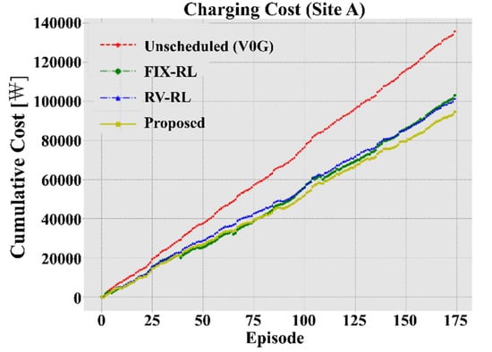
Figure 8.
Cumulative charging cost of the proposed method and the benchmarks for site A.
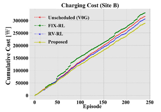
Figure 9.
Cumulative charging cost of the proposed method and the benchmarks for site B.

Table 1.
Cumulative charging cost over total test period in numeric form.
In Table 2, the methods are compared to one another in terms of normalized cost. This is because the four methods charge and discharge differently, meaning the charging costs may differ. Therefore, it is important to compare how much cost is paid per kWh as a result. As shown in Table 2, the proposed method charges at a lower cost than the other methods for both sites.
Table 2.
Normalized total cost over test period.
In Figure 10, an example of scheduling results for several days is presented: (a) shows the actions taken by the trained RL agent. The black line in the figure represents hourly electricity price and the red bars represent the actions. It is observed that the agent has a tendency to charge when the electricity price is low and discharge when the electricity price is high. Notably, that these are not the optimal solution because the agent takes actions considering the trend of the previous price signal rather than knowing the future price. Thus, it can be said these are the best choices to make with only past information given. It can be observed that the actions taken by the agent in Site B are mostly charging actions because the initial energy when EVs arrive at Site B tends to be lower than that of Site A as seen in Figure 6. Hence, our proposed model is not significantly better than the others at Site B. Therefore, the more energy the battery has on arrival, the more room there is a chance to discharge it, thereby leaving more room to save on charging costs.
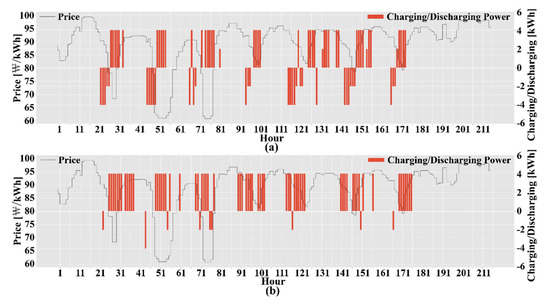
Figure 10.
Scheduling results for several days; (a) site A (b) site B.
4.2.4. Scheduling Effect on a Load Profile
In this section, we discuss how the proposed EV charging and discharging algorithm affects the load profile of the site when it is deployed in chargers. We analyze the load shifting effect numerically by calculating the load factor expressed by Equation (9). The larger load factor means that the difference between the peak and average is small, which means that the load profile is levelized. Conversely, a smaller load factor means that the load profile is not levelized. The calculated results in Table 3 show that the more the number of chargers, the flatter the load profile.
Table 3.
Calculated load factor according to the number of chargers.
We set the target day and analyze how the load profile changes when the charging and discharging of EVs are scheduled by our proposed method with varying number of chargers. The results are shown in Figure 11. The purple line represents the default load profile when unscheduled. The blue, yellow, green, and red dotted lines represent the changed load profile when the number of chargers is set to 1, 5, 10, and 20, respectively. As seen in the figure, as the number of chargers increases, the load shifting effect that can be obtained through scheduling increases also.
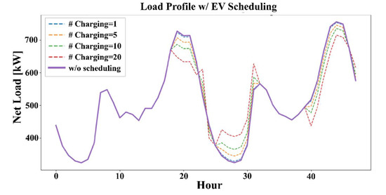
Figure 11.
Load shifting effect when charging and discharging of EVs are scheduled.
Next, we compare the charging methods with our proposed method. Similarly, we compare the results with the load factor, assuming 20 chargers are deployed in the target location. The calculated load factors are in presented in Table 4. In Figure 12, the green line represents the ordinary load profile of the target location without EV chargers. The orange dotted line represents the case where the EVs charge using chargers with the unscheduled method, the blue dotted line represents the FIX-RL method, the purple dotted line represents RV-RL, and the red solid line represents the proposed method. Clearly, with the charging methods other than the proposed method, the EV charging loads are added to the existing load, thus resulting in higher peaks. Otherwise, when our proposed charging and discharging algorithm is deployed in the chargers, the peaks are shaved and the valleys are filled as the yellow line shows. This means the load profile is flattened so that the grid operation is made more reliable.
Table 4.
Calculated load factor of unscheduled method and proposed method.
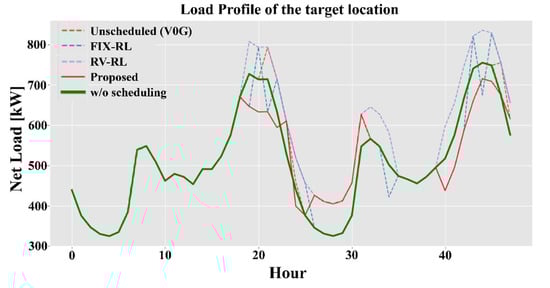
Figure 12.
Comparing benchmark methods and the proposed method in terms of load shifting effect.
To summarize, we analyzed the superiority of our proposed method from two perspectives. First, we calculated the charging cost during the test period and compared that of our proposed method and those of benchmarks. As a result, our proposed method turned out to be superior to the benchmarks in both cumulative charging cost and normalized charging cost. Second, we discussed how the proposed EV charging and discharging algorithm affects the load profile of the site when it is deployed in chargers in this section. The load shifting effect is evaluated by calculating the load factor. We first analyzed the change of the load profile when our proposed method was deployed in chargers. It turned out that there was a load shifting effect, and as the number of chargers increased, the load shifting effect increased as well. Then, with the fixed number of chargers, the load shifting effect of our proposed method was compared to those of the benchmarks. It is obvious that our proposed method outperforms the others in terms of the load factor. Consequently, our proposed method is superior to existing methods, in terms of cost saving and contribution to the peak reduction, if deployed in a specific charger in a specific location.
5. Conclusions
In this study, we discussed a DRL-based algorithm for charging and discharging an EV in response to the hourly electricity price. The proposed method aimed to model the usage pattern of a specific charger in a specific location as a probability distribution, and then use the variables sampled from this probability distribution in the DRL agent to reflect, effectively, the local characteristics. Hence, we proposed a data-driven approach for this task that utilizes a nonparametric density estimation method. We derived probability distributions for the variables related to the charger usage patterns by applying KDE to real-world datasets, and the resulting probability distributions are used to sample those variables to provide a DRL agent with scenarios reflecting the target location. Simulation results show the effectiveness of our proposed method in two ways. First, the proposed method successfully reduces the total charging cost during the test period. Second, our proposed method successfully raised the load factor, which means the load profile of the target location is flattened. This implies that if the proposed algorithm is deployed in many chargers, it will not only save charging costs for users, but also increase the grid reliability. In conclusion, our proposed method is superior to existing methods in terms of cost saving and contribution to the peak reduction if deployed in a specific charger in a specific location. A limitation of this study exists: action space is considered as a discrete space, but there are RL algorithms such as policy gradient that can handle a continuous space. Applying these algorithms can be the future scope.
Author Contributions
All of the authors contributed to this work. J.L. designed the study, performed the literature review, the analysis, and wrote the paper. E.L. contributed to the conceptual approach and thoroughly revised the paper. J.K. led and supervised the research. All authors have read and agreed to the published version of the manuscript.
Funding
This work was supported by the Korea Institute of Energy Technology Evaluation and Planning (KETEP) and the Ministry of Trade, Industry & Energy (MOTIE) of the Republic of Korea (No. 20182010600390).
Conflicts of Interest
The authors declare no conflict of interest.
Abbreviation
| EV | Electric Vehicle |
| ToU | Time-of-Use |
| V2G | Vehicle-to-Grid |
| MDP | Markov Decision Process |
| LSTM | Long Short-Term Memory |
| DRL | Deep Reinforcement Learning |
| SOC | State-of-Charge |
| DQN | Deep Q-Network |
| PEV | Plug-in Electric Vehicle |
| SARSA | State-Action-Reward-State-Action |
| CMDP | Constrained Markov Decision Process |
| SDRL | Safe Deep Reinforcement Learning |
| KDE | Kernel Density Estimation |
Nomenclature
| The state given from the environment at step t | |
| The action taken by the agent at step t | |
| The arrival time | |
| The departure time | |
| The charging duration of EV | |
| The vector of past k-step electricity prices | |
| The reward given from the environment at step t | |
| The 4-tuple of elements of Markov decision process | |
| The amount of energy left in EV battery at t | |
| The amount of energy left until the battery is fully charged at t | |
| The time remaining until the charge is complete at t | |
| The action space given to the agent | |
| The charging/discharging power for k-th level | |
| The capacity of the EV battery | |
| The initial amount of energy left on an arrival of EV | |
| The random variable of and derived by KDE | |
| The random variable of derived by KDE | |
| The kernel function with smoothing parameter h called bandwidth | |
| The action-value function under the policy | |
| The discount factor | |
| The experience replay memory | |
| N | The size of the experience replay memory |
| The network parameter | |
| The learning rate | |
| The loss function | |
| The probability that the agent takes an action depending on the Q-value predicted by the Q-network |
References
- IEA. Global EV Outlook 2019; IEA: Paris, France, 2019. [Google Scholar]
- Clement-Nyns, K.; Haesen, E.; Driesen, J. The impact of charging plug-in hybrid electric vehicles on a residential distribution grid. IEEE Trans. Power Syst. 2009, 25, 371–380. [Google Scholar] [CrossRef]
- Joskow, P.L.; Wolfram, C.D. Dynamic pricing of electricity. Am. Econ. Rev. 2012, 102, 381–385. [Google Scholar] [CrossRef]
- Yang, L.; Dong, C.; Wan, C.J.; Ng, C.T. Electricity time-of-use tariff with consumer behavior consideration. Int. J. Prod. Econ. 2013, 146, 402–410. [Google Scholar] [CrossRef]
- Wang, Q.; Zhang, C.; Ding, Y.; Xydis, G.; Wang, J.; Østergaard, J. Review of real-time electricity markets for integrating distributed energy resources and demand response. Appl. Energy 2015, 138, 695–706. [Google Scholar] [CrossRef]
- Guille, C.; Gross, G. A conceptual framework for the vehicle-to-grid (V2G) implementation. Energy Pol. 2009, 37, 4379–4390. [Google Scholar] [CrossRef]
- Peng, C.; Zou, J.; Lian, L.; Li, L. An optimal dispatching strategy for V2G aggregator participating in supplementary frequency regulation considering EV driving demand and aggregator’s benefits. Appl. Energy 2017, 190, 591–599. [Google Scholar] [CrossRef]
- Thingvad, A.; Calearo, L.; Andersen, P.B.; Marinelli, M.; Neaimeh, M.; Suzuki, K.; Murai, K. Value of V2G frequency regulation in Great Britain considering real driving data. In Proceedings of the 2019 IEEE PES Innovative Smart Grid Technologies Europe, Bucharest, Romania, 29 September–2 October 2019. [Google Scholar]
- White, C.C. Markov Decision Processes; Springer: Berlin, Germany, 2001. [Google Scholar]
- Xie, S.; Zhong, W.; Xie, K.; Yu, R.; Zhang, Y. Fair energy scheduling for vehicle-to-grid networks using adaptive dynamic programming. IEEE Trans. Neural Netw. Learn. Syst. 2016, 27, 1697–1707. [Google Scholar] [CrossRef]
- Tang, W.; Zhang, Y.J. A model predictive control approach for low-complexity electric vehicle charging scheduling: Optimality and scalability. IEEE Trans. Power Syst. 2016, 32, 1050–1063. [Google Scholar] [CrossRef]
- Aragón, G.; Gümrükcü, E.; Pandian, V.; Werner-Kytölä, O. Cooperative control of charging stations for an EV park with stochastic dynamic programming. In Proceedings of the IECON 2019—45th Annual Conference of the IEEE Industrial Electronics Society 2019, Lisbon, Portugal, Portugal, 14–17 October 2019. [Google Scholar]
- Škugor, B.; Deur, J. Dynamic programming-based optimisation of charging an electric vehicle fleet system represented by an aggregate battery model. Energy 2015, 92, 456–465. [Google Scholar]
- Zhang, L.; Li, Y. Optimal management for parking-lot electric vehicle charging by two-stage approximate dynamic programming. IEEE Trans. Smart Grid 2015, 8, 1722–1730. [Google Scholar] [CrossRef]
- Bertsekas, D.P. Dynamic Programming and Optimal Control; Athena Scientific: Belmont, MA, USA, 1995; Volume 1. [Google Scholar]
- Tan, K.M.; Ramachandaramurthy, V.K.; Yong, J.Y. Optimal vehicle to grid planning and scheduling using double layer multi-objective algorithm. Energy 2016, 112, 1060–1073. [Google Scholar] [CrossRef]
- Wang, Z.; Paranjape, R. Optimal scheduling algorithm for charging electric vehicle in a residential sector under demand response. In Proceedings of the 2015 IEEE Electrical Power and Energy Conference (EPEC), London, ON, Canada, 26–28 October 2015; pp. 45–49. [Google Scholar]
- Suyono, H.; Rahman, M.T.; Mokhlis, H.; Othman, M.; Illias, H.A.; Mohamad, H. Optimal scheduling of plug-in electric vehicle charging including time-of-use tariff to minimize cost and system stress. Energies 2019, 12, 1500. [Google Scholar] [CrossRef]
- Yao, L.; Lim, W.H.; Tsai, T.S. A real-time charging scheme for demand response in electric vehicle parking station. IEEE Trans. Smart Grid 2016, 8, 52–62. [Google Scholar] [CrossRef]
- Liu, Z.; Wu, Q.; Ma, K.; Shahidehpour, M.; Xue, Y.; Huang, S. Two-stage optimal scheduling of electric vehicle charging based on transactive control. IEEE Trans. Smart Grid 2018, 10, 2948–2958. [Google Scholar] [CrossRef]
- He, Y.; Venkatesh, B.; Guan, L. Optimal scheduling for charging and discharging of electric vehicles. IEEE Trans. Smart Grid 2012, 3, 1095–1105. [Google Scholar] [CrossRef]
- Ortega-Vazquez, M.A. Optimal scheduling of electric vehicle charging and vehicle-to-grid services at household level including battery degradation and price uncertainty. IET Gen. Trans. Distr. 2014, 8, 1007–1016. [Google Scholar] [CrossRef]
- Jiang, W.; Zhen, Y. A real-time EV charging scheduling for parking lots with PV system and energy storage system. IEEE Access 2019, 7, 86184–86193. [Google Scholar] [CrossRef]
- Ghotge, R.; Snow, Y.; Farahani, S.; Lukszo, Z. Optimized scheduling of EV charging in solar parking lots for local peak reduction under EV demand uncertainty. Energies 2020, 13, 1275. [Google Scholar] [CrossRef]
- Mnih, V.; Kavukcuoglu, K.; Silver, D.; Rusu, A.A.; Veness, J.; Bellemare, M.G.; Graves, A.; Riedmiller, M.; Fidjeland, A.K.; Ostrovski, G. Human-level control through deep reinforcement learning. Nature 2015, 518, 529. [Google Scholar] [CrossRef]
- Wan, Z.; Li, H.; He, H.; Prokhorov, D. Model-free real-time EV charging scheduling based on deep reinforcement learning. IEEE Trans. Smart Grid 2018, 10, 5246–5257. [Google Scholar] [CrossRef]
- Shi, W.; Wong, V.W.S. Real-time vehicle-to-grid control algorithm under price uncertainty. In Proceedings of the 2011 IEEE International Conference on Smart Grid Communications (SmartGridComm), Brussels, Belgium, 17–20 October 2011; pp. 261–266. [Google Scholar]
- Dimitrov, S.; Lguensat, R. Reinforcement learning based algorithm for the maximization of EV charging station revenue. In Proceedings of the 2014 International Conference on Mathematics and Computers in Sciences and in Industry, Varna, Bulgaria, 13–15 September 2014; pp. 235–239. [Google Scholar]
- Vandael, S.; Claessens, B.; Ernst, D.; Holvoet, T.; Deconinck, G. Reinforcement learning of heuristic EV fleet charging in a day-ahead electricity market. IEEE Trans. Smart Grid 2015, 6, 1795–1805. [Google Scholar] [CrossRef]
- Chiş, A.; Lundén, J.; Koivunen, V. Scheduling of plug-in electric vehicle battery charging with price prediction. In Proceedings of the IEEE PES ISGT Europe 2013, Lyngby, Denmark, 6–9 October 2013. [Google Scholar]
- Dang, Q.; Wu, D.; Boulet, B. A Q-learning based charging scheduling scheme for electric vehicles. In Proceedings of the 2019 IEEE Transportation Electrification Conference and Expo (ITEC), Detroit, MI, USA, 19–21 June 2019; pp. 1–5. [Google Scholar]


© 2020 by the authors. Licensee MDPI, Basel, Switzerland. This article is an open access article distributed under the terms and conditions of the Creative Commons Attribution (CC BY) license (http://creativecommons.org/licenses/by/4.0/).