Gene Evaluation Algorithm for Reconfiguration of Medium and Large Size Photovoltaic Arrays Exhibiting Non-Uniform Aging

Abstract

Aging is known to exert various non-uniform effects on photovoltaic (PV) modules within a PV array that consequently can result in non-uniform operational parameters affecting the individual PV modules, leading to a variable power output of the overall PV array. This study presents an algorithm for optimising the configuration of a PV array within which different PV modules are subject to non-uniform aging processes. The PV array reconfiguration approach suggests maximising power generation across non-uniformly aged PV arrays by merely repositioning, rather than replacing, the PV modules, thereby keeping maintenance costs to a minimum. Such a reconfiguration strategy demands data input on the PV module electrical parameters so that optimal reconfiguration arrangements can be selected. The algorithm repetitively sorts the PV modules according to a hierarchical pattern to minimise the impact of module mismatch arising due to non-uniform aging of panels across the array. Computer modelling and analysis have been performed to assess the efficacy of the suggested approach for a variety of dimensions of randomly non-uniformly aged PV arrays (e.g., 5 × 5 and 7 × 20 PV arrays) using MATLAB. The results demonstrate that enhanced power output is possible from a non-uniformly aged PV array and that this can be applied to a PV array of any size.

1. Introduction

Escalating concerns regarding devastating climate changes as a consequence of burning fossil fuels and deforestation have highlighted the importance of developing sustainable energy sources around the globe. Furthermore, non-sustainable fossil fuels constitute a finite resource, and there is an inverse relationship between stock availability (which is declining) and stock price. Consequently, there is an urgent requirement for all energy suppliers to promote energy efficiency and cost-effectiveness to ensure competitiveness in a changing world [1,2].

Photovoltaic (PV) systems represent one of the most popular alternative energy sources. A PV system converts energy from sunlight into electricity and generates no polluting by-products, thus is viewed as a ‘clean’ energy source. Recently, PV systems have become popular both domestically and commercially as a consequence of technological developments leading to reduced electrical losses associated with transmission and distribution, as well the possibility to divert surplus electricity back to the local power utility.

PV systems are particularly common in remote outdoor locations, where they can be exposed to challenging weather conditions and other outdoor hazards such as bird waste. This exposure results in aging that is not necessarily constant across the modules of the array, resulting in degradation of efficiency both in the individual modules and the overall system. However, this non-uniform aging can also be caused by varying characteristics within a module’s cells. The most effective solution to this is the replacement of the affected modules with new equivalents, but this is expensive and may introduce a disparity between the characteristics of the existing and newly introduced modules. This can have a ‘bucket effect’ that prevents the array from producing its optimum power [3,4].

The power of a PV cell is reduced relative to its rated power as it ages. As this can cause a decrease in the cell’s short-circuit current to have a much higher effect than a reduction in its open-circuit voltage, typically the short-circuit current measurement is an indicator of the condition of the cell [5,6]. Due to the non-uniform nature of the aging across the module, it is treated as a trio of submodules of varying age characteristics, in series with each other [7].

Non-uniform aging within a PV array leads to differing electrical characteristics between the PV modules within that array. Replacement of PV modules is costly, so a new way to enhance the power efficiency of aging PV modules is needed [8]. The increased efficiency of PV plants would lead to increased power generation and income, and reduced power generation costs. Therefore, a new approach to reconfigure faulty or aged PV modules would be precious.

A range of approaches has been proposed to enhance PV array output power, mostly in relation to mismatch, including both on- and offline and using both definite and heuristic algorithms. Examples of online approaches to reconfiguring the mismatched PV array to enhance its power efficiency are given in [9,10], but these involve drawbacks such as costly switch and relay requirements and complex calculations. The series–parallel array featured in [3] has just a single short-circuit current per module to indicate its condition, despite the non-uniformly aging process across the modules. This means the calculation requirements are considerably diminished. Therefore, it was decided to enhance the efficiency of the PV array using an offline reconfiguration algorithm.

Initially, a variety of configurations of PV modules within a PV array are possible as depicted in Figure 1: series-parallel (SP), bridge link (BL) and total cross-tied (TCT). The most widely used configurations are SP and TCT [11,12,13,14,15,16,17]. In SP configurations, PV modules are linked in series formation, resulting in strings of modules that can generate the necessary voltage demands of the inverter. These strings are subsequently connected in parallel to form a PV array with the increased total current.

For TCT configurations, PV modules are initially parallel-tied, giving rise to equal voltages across modules and additive current across a row of modules. These module rows may then be connected in series. Although several researchers have examined the performances of various PV array configurations; their configuration selection may vary. For example, some have chosen to examine only essential series and parallel configurations, while others recommended Honey Comb (HC) as the best configuration [18].

Hereon, this method uses the following definitions. A PV array describes a set of PV strings arranged in parallel, themselves formed of PV panels arranged in series. One PV panel comprises either two or three modules arranged in series, themselves formed of PV cells in series with an antiparallel bypass diode [19]. The arrangement is depicted in Figure 2.

An offline reconfiguration approach was suggested in [7] to enhance the energy efficiency of aged PV systems via analysis of the potential options for a reorganisation of PV modules by determining the maximum power point [3]. Alternatively, the genetic algorithm approach used to identify the optimised maximum power output from non-uniformly aged PV modules in an array. Other strategies have demonstrated effectiveness in addressing module rearrangement problems for both small- and large-scale PV arrays, but these required searching all potential combinations of PV rearrangements, resulting in excessive computational complexity and time requirements [3,7]. Another benefit is that only the affected PV modules require repositioning, whereas the others can remain in their original positions. This also has the advantage of keeping the number of relays to be used for switching to a minimum [20,21].

In order to achieve quick calculation with low computing resources, this paper proposes a genetic-algorithm-supported reconfiguration for medium and large PV arrays exhibiting non-uniform aging. Further and in Section 2, the motives for used SP reconfiguration are described. Section 3 system contains a description of the photovoltaic system. In Section 4, the non-uniform-aging Phenomenon. Section 5 contains the reconfiguration scheme of PV array based on gene evolution algorithm (GEA). In Section 6 the simulation results are reported. In Section 7, contains the Outcomes and Conclusion.

2. The Motives for Using SP Reconfiguration

Although several researchers have formulated interconnection topologies, almost all of the solutions that have exploited this, have relied on TCT and SP module interconnections [14]. SP, which comes from strings of interlinked solar modules, is regularly seen in PV power plants. In this technology, strings of interconnected solar modules in series offer the voltage required by the inverter, which is connected in parallel to maximise the total current. In the case of the TCT format, the PV modules are initially parallel-tied, thereby ensuring the following: firstly, that the currents summed, and secondly, that the voltages are the same. In turn, several of the rows of modules are connected in series. In the context of uniform conditions, TCT and SP module connections generate almost identical power values. Under differing conditions, TCT typically performs favourably in terms of energy performance compared to SP [22].

As noted in Section 1, a critical issue that must be considered when addressing re-configurable PV architectures relates to the number of sensors and switches needed, as well as the degree to which the algorithms used for reconfiguration are complex. An especially important issue is that almost every reconfiguration method that relies on TCT topology requires an impractical number of switches and sensors [14]. For instance, for the system developed in [22], the researchers created a switching matrix involving NPV2 double-pole switches with NPV single-pole switches (in this case, N refers to the number of PV modules). It is worth emphasising that a switching matrix of this kind makes it possible to achieve every type of configuration between the two limits of an (a) all parallel-connected modules configuration (every module in one row), and an (b) all-series-connected modules configuration (a single module for each row). Thus, in a system with 24 PV modules, it would be necessary to have 600 switches. To give another example, the switch structure developed in [10] needed 2 ⋅ NPV2 (1152 switches), and almost all of the established reconfiguration techniques relying on the TCT topology necessitate the use of relatively complex control algorithms.

These algorithms are used to ascertain the point at when to switch on or to switch off, but in order to run effectively, they may require an excessive number of calculations [14]. In [22], the potential for a number of total configurations amounting to (NPV * NPV)!/(NPV!)NPV to exist was discussed, and the researchers noted that these must be considered with NPV = 24, since the previous expression results in an overflow in MATLAB. It is clear that, in practice, commercial TCT arrays cannot be easily, effectively and efficiently controlled. The present authors review of the extant evidence suggests that ENDANA, by Bitron, which is the only commercially available device that enables the reconfiguration of a PV array, relies on the SP topology [23]. In the case of the standard version of ENDANA, it can reconfigure 24 PV modules in 2 strings. Additionally, after evaluating the full power vs. voltage (P–V) curve for every PV module and reconfiguring the module connections into two substrings, several strongly shaded PV modules may be excluded.

With the above in mind, this study addresses the SP topology because, theoretically, it can be used to perform a retrofit on almost every current PV field. A key consideration is also that, in nearly every situation, analysis of the reconfiguration of the TCT topology occurs by examining PV units. These PV units can be represented in a straightforward way with strings of PV cells. Additionally, the potential presence of multiple maxima in the P-V features of several strings of this kind should be overlooked. In the case of commercially available PV modules, the protection of every string of cells is achieved using a dedicated bypass diode paired with a partial shadowing that affects the module. This regularly results in the presence of several maximum power point tracking (MPPs). Most studies addressing reconfiguration algorithms for TCT architectures have not considered the issue of the multi-modality of P-V curves.

Additionally, almost every researcher has focused on understanding only of short-circuit currents. Therefore, this study examines a reconfiguration algorithm for the SP connection of commercially available PV modules. It relies on an understanding of the full I–V characteristic of every PV module. This allows it to accurately face the inevitable occurrence of several MPPs in the P-V features of several PV modules. It is worth emphasising that this study’s objective is not to compare the reconfiguration performances of the SP and TCT topologies; rather, the paper seeks to formulate an SP reconfiguration strategy that can be applied to faulty, defective, or aging PV systems, thereby increasing a PV array’s maximum power output by rearranging the positions of the PV module. Specifically, the algorithm proposed in the study must have the ability to determine the ideal configuration in a fast way and to apply it in polynomial time.

3. System Description of the Photovoltaic (PV) Cell and Array

Equivalent circuit models represent the entire I-V curve of a cell/array/module using a continuous function for a specific series of functioning circuit variables. In Figure 3, an overview of the corresponding of a single-diode circuit of the PV cell and the PV modules or array is given [2].

For a single diode, where I_DO is the loss diode current modelled using the Shockley equation for an ideal diode, this can be defined by Equation (1).

$$I_{DO}=I_D\left[\exp \left(\frac{V_{PV}+\left(I_{PV}\cdot R_S\right)q}{n{V}_T}\right)-1\right]$$

(1)

where $V_T$ is the thermal voltage given by the next equation,

$$V_T=\frac{k\cdot T_C}{q}$$

(2)

k is Boltzmann’s constant $1.38\times {10}^{-23}J/K$, T_C in Kelvin is temperature of the p-n junction and the electron charge presented as q $1.6\times {10}^{-19}C$ and n is the ideality factor of the diode which is expressed as:

$$\begin{array}{l}{I}_{PV}=I_{SC}-I_D\left[\exp \left(\frac{V_{PV}+\left(I_{PV}\cdot R_S\right)q}{n{V}_T}\right)-1\right]-\frac{V_{PV}+\left(I_{PV}\cdot R_S\right)}{R_{Sh}}\\ \end{array}$$

(3)

The electrical behaviour of a PV module is modelled using Equation (3), where the ohm’s losses are $R_s$ and $R_{sh}$, I_SC represents the photo-induced current depending on the irradiance, I_D represents the saturation current, nV_T represents the thermal voltage depending on the module temperature, $I_{PV}$ is the current generated by the module. The parameters can be calculated from datasheet values or experimental measurements by solving the expressions given in [2,24].

In the case of a PV array, a set of several PV modules each incorporating in-series electrical linking and parallel circuits is needed. This enables the production of the required current and voltage, and constitutes a PV array. In Figure 2, an illustration is given of the equivalent circuit linked to the PV module with NP parallel-connected cell and NS series-connected cell configuration [2]. Hence, in the case of the PV array, as indicated in Figure 2, it is possible to express the output current equation in the following way:

$$I_{array}=N_p{I}_{SC}-N_p{I}_D{I}_S\left[\exp \left(\frac{ V_{array}+I_{array}\frac{N_s}{N_p}{R}_S(q)}{n{V}_T{N}_s}\right)-1\right]-\frac{V_{array}+I_{array}\frac{N_s}{N_p}{R}_S}{\frac{N_s}{N_p}{R}_{Sh}}$$

(4)

where $N_s$ refers to the cells in series, $N_p$ represents strings in parallel, $V_{Array}$ denotes the bandgap voltage and $I_{Array}$ represents the current. Hence, the reverse saturation (I_S) is the current of the diode, as shown in Equation (4).

Several PV cells connected in series constitute a PV module. Typically a module contains 36 PV cells connected in series. $R_s$ denotes the resistance offered by the solar cells in the path of the current flow. The resistance offered to the leakage current is represented by $R_{sh}$ [25]. The photoelectric current is a function of the short-circuit current and can be expressed as follows

$$I_{SC}=I_{SCm}(1+\alpha (T-T_m))\left(\frac{G}{G_m}\right)\left(\frac{R_S+R_{Sh}}{R_{Sh}}\right)$$

(5)

where is the short circuit-current of the modules $I_{SCm}$ at standard insolation $G_m$ ($1000 \mathrm{W}/{\mathrm{m}}^2$) and standard temperature $T_m$ (25 °C) and α is the module’s temperature coefficient for the current. As seen in Equation (5), the short current-circuit can be defined by the next equation.

$$I_{SCm}=\frac{I_{SC}}{\left(1+\frac{R_S}{R_{Sh}}\right)}$$

(6)

Additionally, the open-circuit voltage can be defined by Equation (6).

$$V_{OC}\approx \left(\frac{n{V}_T}{q}\right)In\left(\frac{I_{SC}}{I_D}\right)$$

(7)

Last, Equation (8) for calculating the solar cell power.

$$P=V\times I=V\times \left(I_{SC}-I_{DO}-\frac{V_{DO}}{R_{Sh}}\right)$$

(8)

Simulation and representation were based on the Solarex MSX60 PV module comprising 36 polycrystalline cells with in-series linking as shown in

Table 1. Parameters for the Solarex MSX60 photovoltaic module at 1000 W/m².

Parameter	Value	Symbols
Open-circuit voltage	21.10 V	VOC
Short-circuit current	3.74 A	ISC
MPP power	60 W	Pmpp
MPP current	3.5 A	Impp
MPP voltage	17.10 V	Vmpp
Cell temperature	25 °C	T

.

An I–V curve is usually used to illustrate the outputs of single-diode PV characteristics [2]. Generally, there are five main parameters to demonstrate PV output characteristics: open-circuit voltage V_OC, short-circuit current I_SC, the voltage at the MPP V_mpp, current at the MPP I_mpp and power at the MPP P_mpp, as shown in Figure 4.

4. The Non-Uniform Aging Phenomenon

A PV generator typically consists of several strings of PV modules arranged in an array. The voltage necessary for the inverter in the grid dictates the number of series-connected (SP) modules assigned to each string, and the grid power supply dictates the number of parallel-connected strings. A representative string PV array layout is shown in Figure 5. In this setup at the right, the voltage across the strings and across the array are the same (V_T), and the current through the array (I_ARRAY) is the aggregate of the currents through the individual strings.

The internal layout of a typical PV module, consisting of a number of series-connected cells, is shown in Figure 5. The setup also includes an anti-parallel-connected bypass diode, which avoids potential negative differences across the PV module that would otherwise cause it to waste power. Figure 5 additionally includes observations of the nonlinear characteristics of a standard-issue Solarex MSX60 module, which exhibits variable output power P_PV that is reliant on the applied voltage V_PV and irradiance S. The output power of the module reaches its peak at a certain point, referred to as the MPPT, under each condition of irradiance [26]. In commercial models, these tend to be continuously tracked by online maximum power point tracker (MPPT) algorithms, due to the variable nature of irradiance.

As shown in the expression and Figure 5, in a short-circuit scenario where V_PV is equal to zero voltage, peak PV current is attained. Equation (3) also infers that the photo-induced current is driving the PV module, and therefore it will always have a current value lower than $I_{SC}$. However, $I_{SC}$ is reliant on the amount of effective irradiance received by the PV module. Therefore if aging is seen across a string of PV modules, they will vary in received irradiance and thus in $I_{SC}$. Although the modules in a PV string are arranged in series and therefore the current through them is equal, a disparity in the $I_{SC}$ values would activate a bypass diode to open a route for the extra current.

An example of this is depicted in Figure 6. The diagram shows a string of a pair of PV modules, one of which is completely exposed to irradiance, and the other of which is partly shielded resulting in smaller $I_{SC}$. In this case, the current in the string has to be less than that photo-induced via the upper module. However, there are two potential operating scenarios. First, a lower current in G1 (I_T < I_SC1) than in the string (I_T > I_SC2) activates the corresponding G2 diode, opening a route for the extra current (I_D G2 = I_T –I_SC2) and causing the negligible voltage across the lower module, so no power is generated. Second, higher current in G2 than in the string (I_T < I_SC1) deactivates the corresponding G1 diode, and power is generated. The point of activation of the bypass diode is referred to as the inflexion point, and the dual-state characteristic overall is referred to as the mismatch phenomenon.

The key indicator of an aging PV string affected by the mismatch phenomenon is that the triggered bypass diodes cause several local maximum power points (LMPP) to appear in the power–voltage (P–V) curve, as shown in Figure 6. The simulated irradiance values are 1000 W/m² at G2 and 600 W/m² at G1, although more pronounced effects have been observed with more significant disparities in irradiance. Also, a substantially higher number of LMPP can appear in the P–V curve in bigger PV arrays, including that shown in Figure 4. In this scenario, for n strings, each consisting of m modules, the number of LMPP is n × m [27].

Several assumptions were accounted for in this section, after which an introduction was given for a suitable model. The 25 aged models will be applied in simulations in the section that follows.

5. Proposed Reconfiguration Algorithm

5.1. PV Array Reconfiguration Scheme

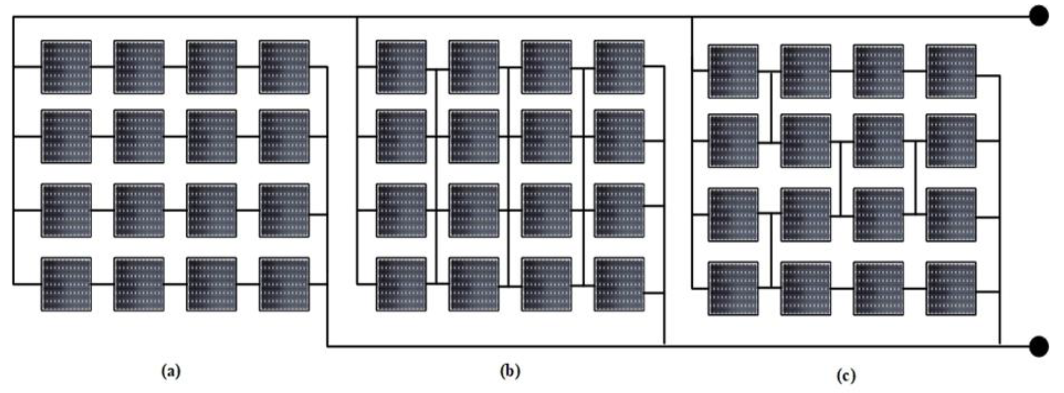
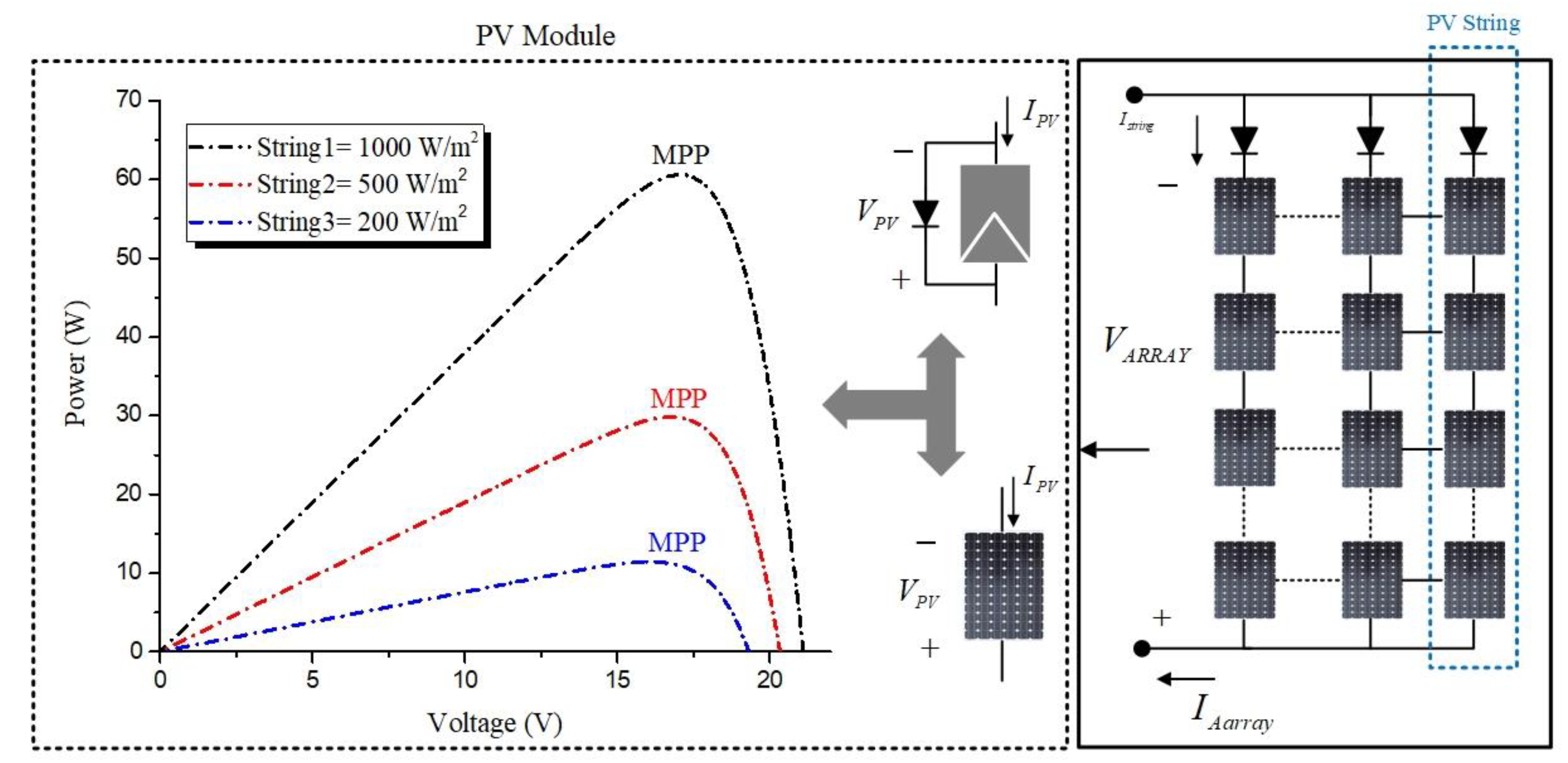
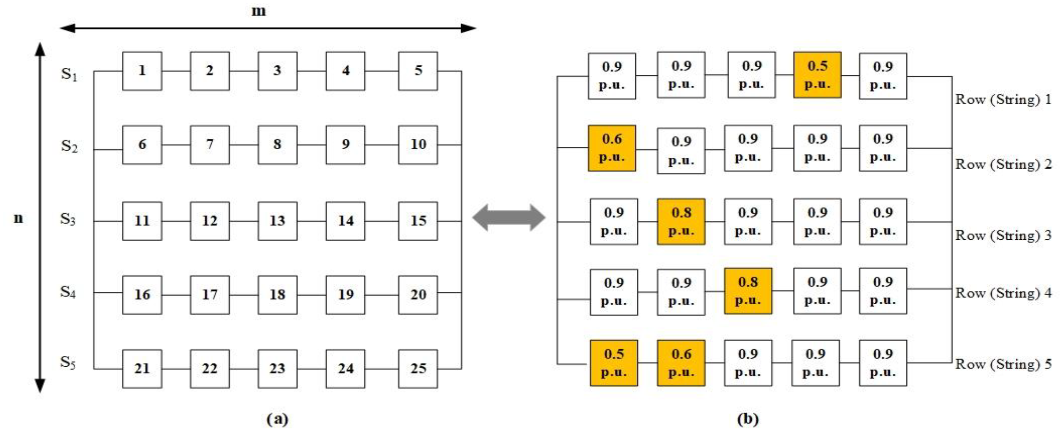
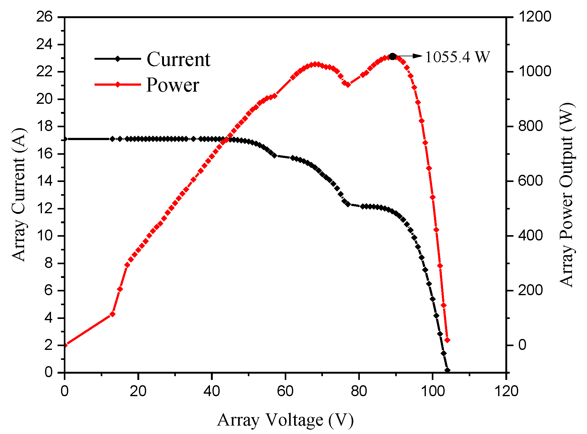
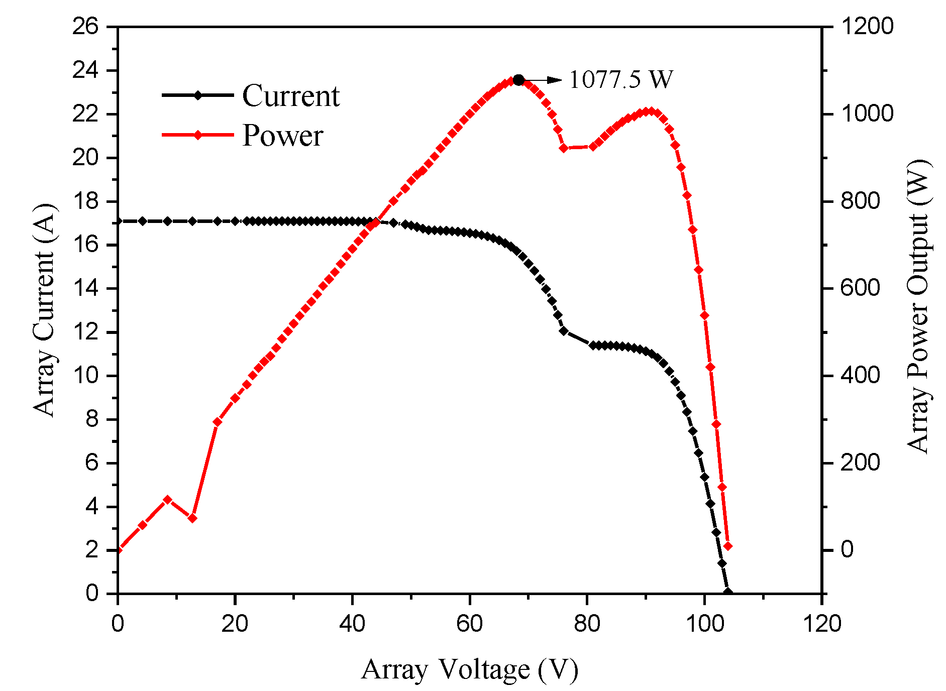
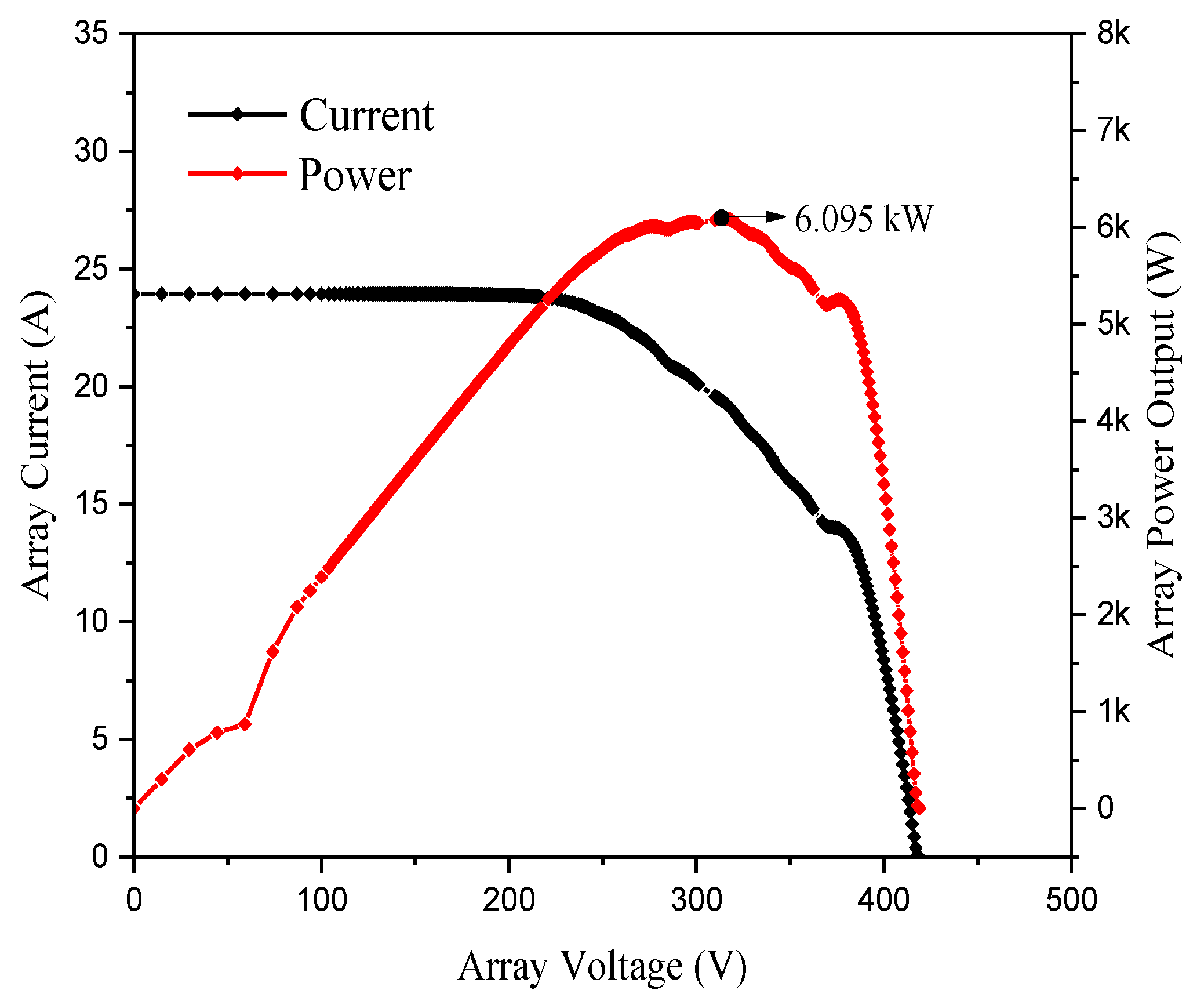
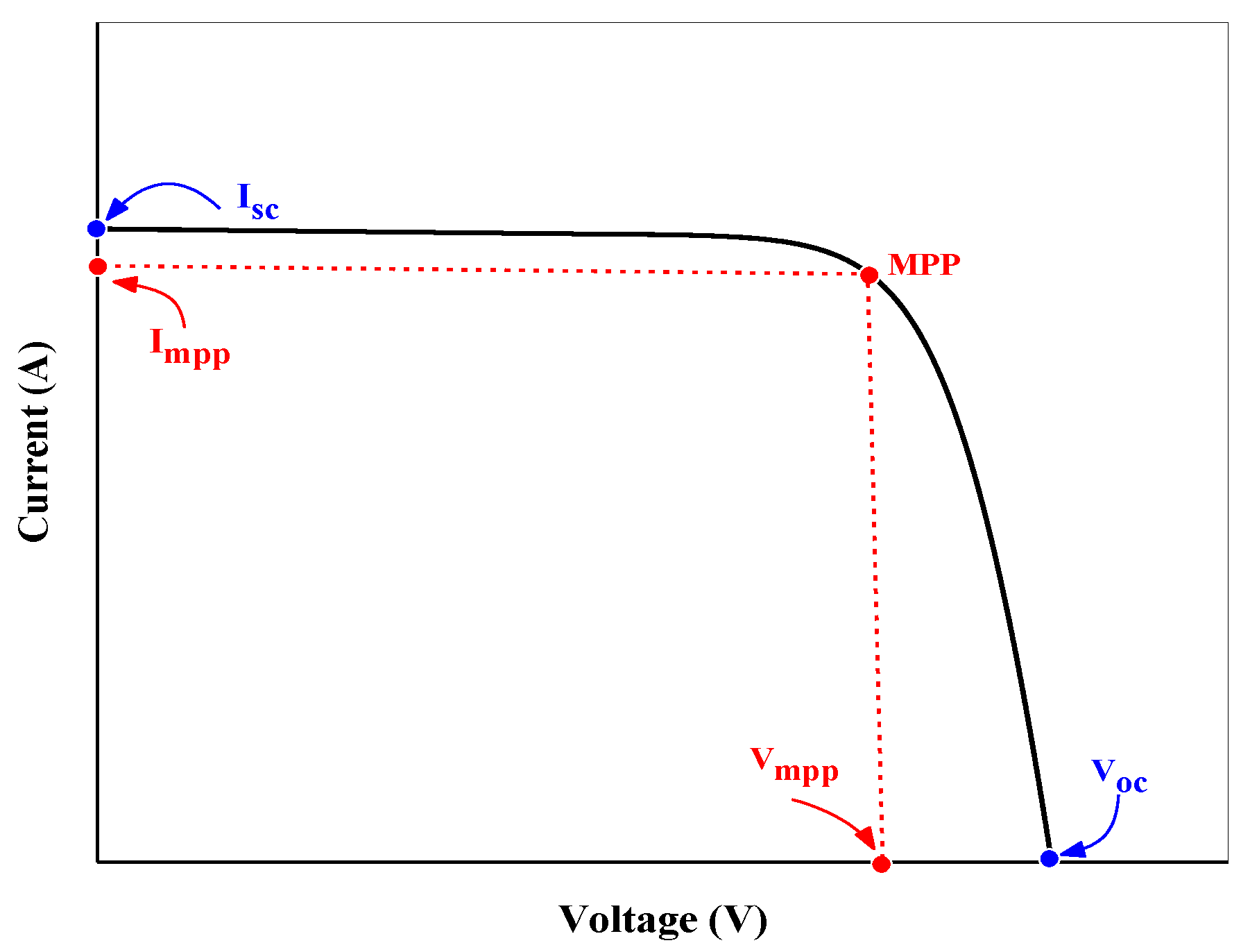
Figure 7a illustrates an n × m PV array where n represents the number of parallel-connected strings and m represents the number of series-connected PV modules per string. The voltage at the GMPP of a PV array in the P–V curve indicates the number of active modules for a given string voltage. Consequently, the maximum power of the PV array can be derived from the product of the sum of all string currents multiplied by the string voltage of all the active modules.

A PV array comprising 25 aged modules connected in a 5 × 5 SP configuration (depicted in Figure 7) will be utilised to demonstrate this concept. Note, that in Figure 7, the array comprises five parallel-connected strings (rows) and five series-connected modules (columns). At the same time, the per-unit values give the non-uniform-aging status of the PV array, which is directly correlated with their individual short-circuit currents.

In a suitable module, the standard test condition (STC) specify the short-circuit current to be 1 per-unit (p.u.), which corresponds to 1000 W/m². The digits indicate the various aging factors (AF) associated with the PV modules in the array, that are directly correlated with their separate short-circuit current. For instance, the optimisation issue is addressed in the present work based on a GEA, which is applied to a 5 × 5 PV array arrangement in Figure 7. Therefore, before presenting the two steps of the suggested algorithm, several parameters need to be described to elucidate the rearrangement work listed below. There are two rules suggested for this work before and after arrangements.

Before presenting the nine steps of the suggested algorithm, several parameters need to be described to elucidate the rearrangement work listed below.

• n = 1, 2, 3…, n, n − 1, where the number of strings in the PV array called n.
• ${\displaystyle \sum Af}$ = Summation of aging factors in a series of connected modules.
• $m_{min(n)}$ = $A{f}_n$ in a series-connection for a string (n)
• $m_{max(n)}$ = $A{f}_n$ in a series-connection for a string (n + 1).
• $P{V}_{n(min)}$ = position of PV module with a minimum $A{f}_n$ in a series of connected modules.
• $P{V}_{n(max)n+1}$ = position of PV module with a maximum $A{f}_n$ in a series of connected modules.

First step: initialize the summation of $P{V}_n=A{f}_n$ for each string before arrangement, as follows in Figure 8 and Equation (9):

$$\begin{array}{lll}P{V}_n=& \begin{array}{l}{\displaystyle \sum A{f}_1=0.9+0.9+0.9+0.5+0.9}=4.1\\ {\displaystyle \sum A{f}_2=0.6+0.9+0.9+0.9+0.9}=4.2\\ {\displaystyle \sum A{f}_3=0.9+0.8+0.9+0.9+0.9}=4.4\\ {\displaystyle \sum A{f}_4=0.9+0.9+0.8+0.9+0.9}=4.4\\ {\displaystyle \sum A{f}_5=0.5+0.6+0.9+0.9+0.9}=3.8\end{array}& p.u.\end{array}$$

(9)

Second step: the rule specifies that, in a string, the minimal number represents the $A{f}_n$ output. This means that the output is the lowest among all values from high to low. Arrange all the $P_n=A{f}_n\times P{V}_n$ before arrangement in descending order to find the total of PV₅, PV4 … and PV₁, presented in Equations (10)–(12) for the case study.

$$P{V}_5=\left(\begin{array}{l}{S}_1=0.5\times 5=2.5\\ S_2=0.6\times 5=3\\ S_3=0.8\times 5=4\\ S_4=0.8\times 5=4\\ S_2=0.5\times 5=2.5\end{array}\right)p.u. \mathrm{and} P{V}_4=\left(\begin{array}{l}{S}_1=0.9\times 4=3.6\\ S_2=0.9\times 4=3.6\\ S_3=0.9\times 4=3.6\\ S_4=0.9\times 4=3.6\\ S_2=0.6\times 4=2.4\end{array}\right)p.u.$$

(10)

$$P{V}_3=\left(\begin{array}{l}{S}_1=0.9\times 3=2.7\\ S_2=0.9\times 3=2.7\\ S_3=0.9\times 3=2.7\\ S_4=0.9\times 3=2.7\\ S_2=0.9\times 3=2.7\end{array}\right)p.u. \mathrm{and} P{V}_2=\left(\begin{array}{l}{S}_1=0.9\times 3=2.7\\ S_2=0.9\times 3=2.7\\ S_3=0.9\times 3=2.7\\ S_4=0.9\times 3=2.7\\ S_2=0.9\times 3=2.7\end{array}\right)p.u.$$

(11)

$$P{V}_1=\left(\begin{array}{l}{S}_1=0.9\\ S_2=0.9\\ S_3=0.9\\ S_4=0.9\\ S_2=0.9\end{array}\right)p.u.$$

(12)

5.2. Optimal Reconfiguration Based on GEA

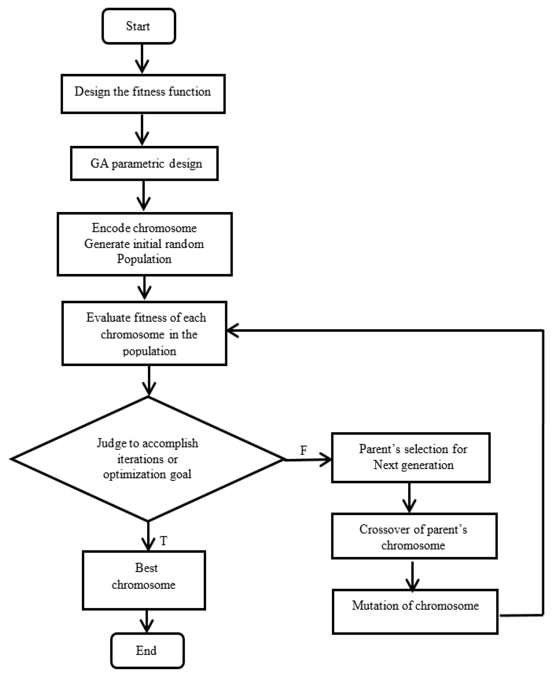
A gene evaluation algorithm is applied to determine the configuration which has the maximum generated power among all possible connection patterns. The genetic algorithm has two significant advantages: firstly, it allows the genetic algorithm to have a certain degree of local random searchability. When the iteration is close to a better solution for a certain number of times, the convergence to a better solution can be accelerated through mutation operations. Secondly, it can maintain that the diversity of feasible solutions can prevent the appearance of precocity. To use GEA, each configuration must be represented by a row of numbers that play a role as a chromosome in GEA. Also, there must be a fitness function to calculate the power generated by each configuration. The inputs of fitness function are chromosomes prepared before. Then according to outputs of the fitness function, GEA decides which chromosomes should be selected as parents to produce chromosomes of the next generation. Therefore, in order to do optimisation for this problem, the following steps must be done.

$${\mathrm{n} \times \mathrm{m} }_{\mathrm{matrix}}=\left[\begin{array}{ccccc}0.9& 0.9& 0.9& 0.5& 0.9\\ 0.6& 0.9& 0.9& 0.9& 0.9\\ 0.9& 0.8& 0.9& 0.9& 0.9\\ 0.9& 0.9& 0.8& 0.9& 0.9\\ 0.5& 0.6& 0.9& 0.9& 0.9\end{array}\right]$$

(13)

First step: the fitness function was designed as a normalised quantity. Equation (14) describes the proposed fitness function $P{V}_i$ Equation (14), where $S_n=A{f}_1+A{f}_2+A{f}_3+A{f}_4+A{f}_5$ represent the short-circuit current of the modules, $V_{OC}$ represents the open-circuit voltage,$P{V}_{power}$ represents the power delivered by the PV array and $n_{PV}$ represent the number of modules in the system. Therefore, the objective of the GEA is to maximise the value of $P{V}_i$ as much as possible.

$$P{V}_i=\frac{P{V}_{pwoer}}{{\displaystyle \sum _{j=1}^{n_{PV}}{S}_{n(j)}·V_{OC}}}$$

(14)

Second step: parametric design based on three points:

• Population size count $=300$
• Chromosome length $= \mathrm{nm}$
• Evolution times $=3000$

Third step: the encoding strategy uses a decimal. Directly encode with the number of the PV module. For example, the chromosome can be expressed as the sequence $\left\{1, 2, 3\dots \mathrm{nm}\right\}$.

Initialise the random population. In order to speed up the running of the program, some better individuals should be selected in the initial population selection. We first use the improved circle algorithm to obtain a better initial population. The idea of the algorithm is to randomly generate a chromosome, such as $\left\{1, 2, 3\dots \mathrm{nm}\right\}$, and exchange the sequential position of the two modules arbitrarily. Continue the following two to convert a one-dimensional list into a two-dimensional matrix. If the value of the $P{V}_i$ that needs to be optimised increases, the chromosome is updated and changed.

Fourth step: evaluate the fitness of each chromosome in the population. The chromosome is transformed into a two-dimensional array ($\mathrm{nm})$. Then according to the fitness function designed, calculate $P{V}_i$.

Fifth step: judge to accomplish iterations or optimisation goal. If successful, then go to step nine, else go to step six.

Sixth step: parent’s selection for next-generation. Firstly, to select the surviving chromosomes, the fitness is sorted from large to small, then the random selection is performed to select individuals who have small fitness but survive.

Seventh step: crossover of parent’s chromosome. The crossover strategy is the difficulty of this problem. If the point cross is used directly, the offspring chromosomes will have the issues of PV- model duplication and omission. Therefore the order crossover method is used. The sequential hybridisation algorithm first randomly selects two hybridisation points among parents and then exchanges hybridisation segments. The other positions are determined according to the relative positions of the parents’ models.

For example, the chromosome can be expressed as the sequence $\left\{1, 2, \dots ,10\right\}$. Suppose:

Parent one =$\left\{10, 8, 6, 3, 7, 4, 1, 5, 9, 2\right\}$

Parent two = $\left\{1, 5, 10, 6, 9, 8, 2, 4, 3, 7\right\}$. Then the random hybridisation points are 4 and 7. As shown in

Table 2. Two chromosomes and the random hybridisation point are set to 4 and 7.

Parent one’	10	8	6	3	7	4	1	5	9	2
Parent two’	1	5	10	6	9	8	2	4	3	7

.

First, swap the hybrids as shown in

Table 3. Swap substrings in parents.

Parent one’	#	#	#	#	9	8	2	4	#	#
Parent two’	#	#	#	#	7	4	1	5	#	#

:

Parent one’ = $\left\{\#, \#, \#, \#, \left| 9, 8, 2, 4 \right|, \#, \#\right\}$

Parent two’= $\left\{\#, \#, \#, \#, \left| 7, 4, 1, 5 \right|, \#, \#\right\}$

And then starting from the second hybridisation point of parent one, getting the collection $\left\{9, 2, 10, 8, 6, 3, 7, 4, 1, 5\right\}$; then removing the elements in the hybridisation segment $\left\{9, 8, 2, 4\right\}$, finally obtaining $\left\{10, 6, 3, 7, 1, 5\right\}$, match the hybridisation point 7 filled in parent one’, at last, parent one’=$\left\{3, 7, 1, 5, 9, 8, 2, 4, 10, 6\right\}$ from the second crossing point in turn. Similarly, parent two’= $\left\{4, 9, 10, 2, 7, 3, 1, 6, 8, 5\right\}$. As shown in

Table 4. Crossover of parents chromosomes.

Parent one’	3	7	1	5	9	8	2	4	10	6
Parent two’	6	9	8	2	7	4	1	5	3	10

.

Eighth step: mutation of chromosome. Mutation is also a means to achieve group diversity, as well as a guarantee for global optimisation. The specific design is as follows. According to the given mutation rate, for the selected mutant individuals, three integers are randomly taken to satisfy $1 < \mathrm{u} < \mathrm{v} < \mathrm{w} < \mathrm{nm}$ and the genes between v and u (including u and v) the paragraph is inserted after w. Then we go to step four.

Final step: output the best chromosome. The optimal configuration for the PV array is displayed in the last step of Figure 9. Equation (15) demonstrates how each configuration that reached each step is compared with the original configuration. The optimal configuration for a non-uniformly aging 5 × 5 PV array took just nine iterations to achieve. The optimal configuration for a large PV array is calculated with the assistance of MATLAB Intel (R) Core (7M) i7-8565u CPU @1.80 GHZ/windows 10/8 GB/512gb SSD/UHD 620to be the one given after enhancement. Therefore, the reconfigured 5 × 5 PV array is the optimal configuration. Figure 8 shows the before and after reconfiguration PV arrays for direct comparison.

$$\begin{array}{lll}P{V}_n=& \begin{array}{l}{\displaystyle \sum A{f}_1=0.9+0.5+0.9+0.9+0.9}=4.1\\ {\displaystyle \sum A{f}_2=0.9+0.9+0.9+0.8+0.9}=4.4\\ {\displaystyle \sum A{f}_3=0.9+0.5+0.9+0.8+0.9}=4\\ {\displaystyle \sum A{f}_4=0.9+0.6+0.9+0.9+0.9}=4.2\\ {\displaystyle \sum A{f}_5=0.9+0.6+0.9+0.9+0.9}=4.2\end{array}& p.u.\end{array}$$

(15)

6. Case Studies

To demonstrate validation of the proposed algorithm, a number of PV arrays of different sizes will be evaluated 5 × 5 and 7 × 20 PV arrays. The maximum power outputs from these PV configurations, both before and after arrangements, are determined by the employment of a PV array model constructed in MATLAB Intel (R) Core (7M) i7-8565u CPU @1.80 GHZ/Windows 10/8 GB/512 gb SSD/UHD 620 which employed to carry out the calculations. The corresponding computing times for 5 × 5 and 7 × 20 PV arrays were arranged.

6.1. Case 1 (5 × 5 PV Array)

Verification of the results using MATLAB can be obtained from Figure 8. The maximum short-circuits currents in a healthy module is set as 1 p.u. (STC), where standard test conditions represent 1000 W/m² irradiance at 25 °C module temperature. The reconfiguration of the PV array via the developed algorithm is presented in

Table 5. Arrangement of the first PV array before and after reconfiguration.

Before					After
0.9 p.u.	0.9 p.u.	0.9 p.u.	0.5 p.u.	0.9 p.u.	0.9 p.u.	0.5 p.u.	0.9 p.u.	0.9 p.u	0.9 p.u.
0.6 p.u.	0.9 p.u.	0.9 p.u.	0.9 p.u.	0.9 p.u.	0.9 p.u.	0.9 p.u.	0.9 p.u.	0.8 p.u.	0.9 p.u.
0.9 p.u.	0.8 p.u.	0.9 p.u.	0.9 p.u.	0.9 p.u.	0.9 p.u.	0.5 p.u.	0.9 p.u.	0.8 p.u.	0.9 p.u.
0.9 p.u.	0.9 p.u.	0.8 p.u.	0.9 p.u.	0.9 p.u.	0.9 p.u.	0.6 p.u.	0.9 p.u.	0.9 p.u.	0.9 p.u.
0.5 p.u.	0.6 p.u.	0.9 p.u.	0.9 p.u.	0.9 p.u.	0.9 p.u.	0.6 p.u.	0.9 p.u.	0.9 p.u.	0.9 p.u.

. Based on this data, Figure 10 and Figure 11 display corresponding I–V and P–V curves. Figure 10 shows that before the reconfiguration the peak output power and voltage were 1055.4 W and 89 V, respectively, with global maximum power point (GMPP) current 11.8 A. Figure 11 shows that after the reconfiguration these were 1077.5 W and 68 V, respectively, with GMPP current 15.73 A. Clearly, the algorithm has enabled an overall improvement of 2.08% to the output power. As shown in

Table 6. The 5 × 5 PV array parameters before and after arrangement.

Parameters	Before	After	Power Improvement	Computing Time (s)
Current GMPP	11.8 A	15.73 A
Voltage GMPP	89 V	68 V	2.08%	0.015625
Power GMPP	1055.4 W	1077.5 W

, the total time to compute the reconfiguration was 0.015625 s.

6.2. Case (7 × 20 PV Array)

Here, non-uniform aging factors were randomly generated for a large 7 × 20 PV array, comprising twenty parallel-connected strings and seven series-connected modules. The aging factors, ranging from 0.9 p.u. to 0.5 p.u. as shown in

Table 7. PV array before arrangement for second case.

Before

0.9 p.u.

0.9 p.u.

0.9 p.u.

0.6 p.u.

0.9 p.u.

0.5 p.u.

0.9 p.u.

0.9 p.u.

0.6 p.u.

0.9 p.u.

0.9 p.u.

0.9 p.u.

0.9 p.u.

0.9 p.u.

0.9 p.u.

0.8 p.u.

0.9 p.u.

0.9 p.u.

0.9 p.u.

0.6 p.u.

0.8 p.u.

0.9 p.u.

0.9 p.u.

0.9 p.u.

0.5 p.u.

0.9 p.u.

0.9 p.u.

0.9 p.u.

0.9 p.u.

0.9 p.u.

0.6 p.u.

0.9 p.u.

0.9 p.u.

0.5p.u.

0.9 p.u.

0.9 p.u.

0.9 p.u.

0.9 p.u.

0.9 p.u.

0.9 p.u.

0.9 p.u.

0.9 p.u.

0.5p.u.

0.9 p.u.

0.8 p.u.

0.9 p.u.

0.9 p.u.

0.8 p.u.

0.8 p.u.

0.9 p.u.

0.6 p.u.

0.9 p.u.

0.9 p.u.

0.9 p.u.

0.9 p.u.

0.9 p.u.

0.9 p.u.

0.9 p.u.

0.9 p.u.

0.9 p.u.

0.9 p.u.

0.5 p.u.

0.9 p.u.

0.5 p.u.

0.5 p.u.

0.9 p.u.

0.9 p.u.

0.9 p.u.

0.9 p.u.

0.9 p.u.

0.9 p.u.

0.9 p.u.

0.9 p.u.

0.6 p.u.

0.6 p.u.

0.9 p.u.

0.9 p.u.

0.9 p.u.

0.9 p.u.

0.8p.u.

0.8 p.u.

0.8 p.u.

0.9 p.u.

0.9 p.u.

0.9 p.u.

0.9 p.u.

0.9 p.u.

0.9 p.u.

0.9 p.u.

0.9 p.u.

0.9 p.u.

0.9 p.u.

0.9 p.u.

0.8 p.u.

0.9 p.u.

0.9 p.u.

0.9 p.u.

0.9 p.u.

0.5 p.u.

0.9 p.u.

0.9 p.u.

0.9 p.u.

0.9 p.u.

0.9 p.u.

0.9 p.u.

0.9 p.u.

0.9 p.u.

0.9 p.u.

0.9 p.u.

0.9 p.u.

0.9 p.u.

0.6 p.u.

0.9 p.u.

0.9 p.u.

0.9 p.u.

0.9 p.u.

0.9 p.u.

0.6 p.u.

0.9 p.u.

0.9 p.u.

0.9 p.u.

0.9 p.u.

0.9 p.u.

0.8 p.u.

0.9 p.u.

0.9 p.u.

0.9 p.u.

0.8 p.u.

0.9 p.u.

0.9 p.u.

0.9 p.u.

0.9 p.u.

0.9 p.u.

0.9 p.u.

0.6 p.u.

0.9 p.u.

0.9 p.u.

0.9 p.u.

0.9 p.u.

0.9 p.u.

After

0.9 p.u.

0.9 p.u.

0.8 p.u.

0.9 p.u.

0.9 p.u.

0.9 p.u.

0.9 p.u.

0.9 p.u.

0.8 p.u.

0.5 p.u.

0.8 p.u.

0.9 p.u.

0.9 p.u.

0.9 p.u.

0.8 p.u.

0.8 p.u.

0.9 p.u.

0.9 p.u.

0.9 p.u.

0.9 p.u.

0.9 p.u.

0.9 p.u.

0.9 p.u.

0.9 p.u.

0.9 p.u.

0.9 p.u.

0.9 p.u.

0.9 p.u.

0.9 p.u.

0.6 p.u.

0.9 p.u.

0.9 p.u.

0.9 p.u.

0.9 p.u.

0.9 p.u.

0.9 p.u.

0.9 p.u.

0.9 p.u.

0.9 p.u.

0.9 p.u.

0.9 p.u.

0.9 p.u.

0.9 p.u.

0.9 p.u.

0.9 p.u.

0.9 p.u.

0.9 p.u.

0.9 p.u.

0.9 p.u.

0.9 p.u.

0.9 p.u.

0.9 p.u.

0.9 p.u.

0.9 p.u.

0.6 p.u.

0.9 p.u.

0.9 p.u.

0.9 p.u.

0.9 p.u.

0.9 p.u.

0.8 p.u.

0.9 p.u.

0.9 p.u.

0.5 p.u.

0.9 p.u.

0.8 p.u.

0.9 p.u.

0.9 p.u.

0.9 p.u.

0.9 p.u.

0.8 p.u.

0.9 p.u.

0.9 p.u.

0.9 p.u.

0.9 p.u.

0.9 p.u.

0.9 p.u.

0.9 p.u.

0.9 p.u.

0.8 p.u.

0.6 p.u.

0.9 p.u.

0.5 p.u.

0.5 p.u.

0.5 p.u.

0.5 p.u.

0.9 p.u.

0.9 p.u.

0.9 p.u.

0.6 p.u.

0.6 p.u.

0.8 p.u.

0.6 p.u.

0.6 p.u.

0.9 p.u.

0.6 p.u.

0.5 p.u.

0.5 p.u.

0.6 p.u.

0.9 p.u.

0.8 p.u.

0.9 p.u.

0.9 p.u.

0.9 p.u.

0.9 p.u.

0.9 p.u.

0.9 p.u.

0.9 p.u.

0.9 p.u.

0.9 p.u.

0.9 p.u.

0.9 p.u.

0.9 p.u.

0.9 p.u.

0.9 p.u.

0.9 p.u.

0.9 p.u.

0.9 p.u.

0.9 p.u.

0.9 p.u.

0.9 p.u.

0.9 p.u.

0.9 p.u.

0.6 p.u.

0.9 p.u.

0.9 p.u.

0.9 p.u.

0.9 p.u.

0.9 p.u.

0.9 p.u.

0.9 p.u.

0.9 p.u.

0.9 p.u.

0.9 p.u.

0.9 p.u.

0.9 p.u.

0.9 p.u.

0.9 p.u.

0.9 p.u.

0.9 p.u.

, were randomly generated, as in the second case. A power improvement of 9.74% was observed following the application of the proposed algorithm, as presented in

Table 8. PV array 7 × 20 parameters before and after arrangement.

Parameters	Before	After	Power Improvement	Computing Time (s)
Current GMPP	19.38 A	20.4 A
Voltage GMPP	314 V	329 V	9.74%	0.129375
Power GMPP	6.095 W	6.721 kW

, I–V and P–V curves were plotted as depicted in Figure 12 and Figure 13 with a mean computational time of 0.129375 s.

7. Outcomes and Conclusions

These findings demonstrate that the proposed algorithm applies randomly to various PV array sizes. The findings also indicate that the algorithm improved maximum power output for both cases. Additionally, the algorithm reduced the impact of the bypass diodes by rearranging the positions of separate PV modules in each string, based on their appropriate aging factors. This minimised the impact of mismatch losses over PV modules in any specified string, but voltage limitation was not taken into consideration. However, this has been discussed elsewhere in the literature [7]. The proposed algorithm utilises a hierarchical and iterative sorting of PV modules. The resulting P−V curves for the two worked examples, as presented in Figure 10, Figure 11, Figure 12 and Figure 13, demonstrate that the influence of PV module mismatch reduced before rearrangement. From case 1 as an example, comparing the maximum power point with maximum power 1077.5 W improved significantly, which concludes that PV array rearrangement is an important method to improve system efficiency and decrease system operation cost.

Furthermore, there is no requirement for the proposed algorithm to access every possible on- offline configuration for any specified PV array, which would be a massive undertaking. This is what enables the algorithm to produce results relatively quickly. For example, in case 1, only nine steps were required for the algorithm to identify the optimum PV module arrangement, and so there was no requirement to analyse huge numbers of arrangements. Relevant computational times for the two cases are reported in Table 4 and Table 6. Therefore, the proposed algorithm can quickly determine the optimal module configuration, which can then also be implemented quickly in real-time. Another advantage is that the affected PV modules are the only ones that require rearrangement, while the rest can remain in their original positions. This has the additional benefit of keeping the number of relays required for switching purposes to a minimum, thereby offering cost and time savings compared to other approaches [3,7,28,29]. It is worth bearing in mind, however, that the prohibitive expense associated with the number of switches and cables required for this method make it impractical. Achieving online reconfiguration with electric switches would necessitate the use of countless switches and cables, which corresponds to a prohibitive cost for real-world applications. Therefore, the offline optimal reconfirmation is more comfortable with calculating, without a need for high-performance controllers. A summary of online and offline reconfiguration methods as shown in

Table 9. Comparison of offline and online reconfiguration methods.

Item	Online Reconfiguration	Offline Reconfiguration
Health monitoring	Real-time monitoring	Periodic monitoring
Implementations of reconfiguration	On-site switching reconfiguration	Manual connection
Computation of reconfiguration	On-site computation with powerful controllers	Offline computation
Applicable array	Small-scale PV arrays	Any arrays

.

In conclusion, the phenomenon of non-uniform aging is prevalent in large-scale PV plants due to the long period of service required and the harsh environments PV arrays are exposed to. Therefore, this study derived a modelling and computing GEA that simulates and analyses the possible rearrangement of aging PV arrays and the resulting output power. A non-linear integer programming solution was devised to improve power output by rearranging the PV panels. Voltage restrictions were taken into account and a 5 × 5 and a 7 × 20 PV array was used to test and prove the devised algorithm. Thus, the maximum power output was increased by 2.08% for the first case, and by 9.74% for the second case. When comparatively examined with the current online PV array reconfiguration techniques, the proposed method does not need as many relays, and it also enhances the maximum power output of the PV system. At the same time, because the algorithm necessitates only that the positions of the PV modules are switched around, it can be implemented straightforwardly.

This rearrangement offered an efficient maintenance management. The plan for offline reconfiguration is dependent on issues such as the benefit and the cost. Generating a PV plant’s ageing map is critical, which makes it necessary to devise offline a reconfiguration technique for calculating the improvement in efficiency, profitability and the workforce cost for reconfiguration. If the profit gained from generating greater amounts of power can pay for the costs associated with the reconfiguration of the workforce, then it is reasonable to conclude that the owner of a PV plant should undertake a reconfiguration to leverage the advantageous aspects of this practice. In view of these considerations, the benefit of the proposed strategy involves employing a workforce to swap PV modules positions only.

References

1. Yadav, A.S.; Pachauri, R.K.; Chauhan, Y.K.; Choudhury, S.; Singh, R. Performance enhancement of partially shaded PV array using novel shade dispersion effect on magic-square puzzle configuration. Sol. Energy 2017, 144, 780–797. [Google Scholar] [CrossRef]
2. Alkahtani, M.; Wu, Z.; Kuka, C.S.; Alahammad, M.S.; Ni, K. A Novel PV Array Reconfiguration Algorithm Approach to Optimising Power Generation across Non-uniformly Aged PV Arrays by merely Repositioning. J.—Multidiscip. Sci. J. 2020, 3, 32–53. [Google Scholar] [CrossRef] [Green Version]
3. Hu, Y.; Zhang, J.; Wu, J.; Cao, W.; Tian, G.Y.; Kirtley, J.L. Efficiency Improvement of Nonuniformly Aged PV Arrays. IEEE Trans. Power Electron. 2017, 32, 1124–1137. [Google Scholar] [CrossRef] [Green Version]
4. Abedi, O.; Hatami, A. A Rearrangement Strategy for a Non-Uniformly-Aged PV Array Using a Modified PGenetic Algorithm. In Proceedings of the 2019 27th Iranian Conference on Electrical Engineering (ICEE), Yazd, Iran, 30 April–2 May 2019; pp. 635–640. [Google Scholar]
5. Osterwald, C.R.; Anderberg, A.; Rummel, S.; Ottoson, L. Degradation analysis of weathered crystalline-silicon PV modules. In Proceedings of the Conference Record of the Twenty-Ninth IEEE Photovoltaic Specialists Conference, New Orleans, LO, USA, 19–24 May 2002; pp. 1392–1395. [Google Scholar]
6. Munoz, M.A.; Alonso-García, M.C.; Vela, N.; Chenlo, F. Early degradation of silicon PV modules and guaranty conditions. Sol. Energy 2011, 85, 2264–2274. [Google Scholar] [CrossRef]
7. Hu, Y.; Zhang, J.; Li, P.; Yu, D.; Jiang, L. Non-Uniform Aged Modules Reconfiguration for Large-Scale PV Array. IEEE Trans. Device Mater. Reliab. 2017, 17, 560–569. [Google Scholar] [CrossRef] [Green Version]
8. Liu, J.; Yao, Y.; Xiao, S.Q.; Gu, X. Review of status developments of high-efficiency crystalline silicon solar cells. J. Phys. D 2018, 51, 12. [Google Scholar] [CrossRef]
9. Velasco-Quesada, G.; Guinjoan-Gispert, F.; Pique-Lopez, R.; Roman-Lumbreras, M.; Conesa-Roca, A. Electrical PV Array Reconfiguration Strategy for Energy Extraction Improvement in Grid-Connected PV Systems. IEEE Trans. Ind. Electron. 2009, 56, 4319–4331. [Google Scholar] [CrossRef] [Green Version]
10. Storey, J.; Wilson, P.R.; Bagnall, D. The Optimized-String Dynamic Photovoltaic Array. IEEE Trans. Power Electron. 2014, 29, 1768–1776. [Google Scholar] [CrossRef] [Green Version]
11. Mekhilef, S.; Saidur, R.; Kamalisarvestani, M. Effect of dust, humidity and air velocity on efficiency of photovoltaic cells. Renew. Sustain. Energy Rev. 2012, 16, 2920–2925. [Google Scholar] [CrossRef]
12. Cristaldi, L.; Faifer, M.; Rossi, M.; Toscani, S.; Catelani, M.; Ciani, L.; Lazzaroni, M. Simplified method for evaluating the effects of dust and aging on photovoltaic panels. Measurement 2014, 54, 207–214. [Google Scholar] [CrossRef]
13. Sankar, M.; Ramabadran, R. Comprehensive analysis on the role of array size and configuration on energy yield of photovoltaic systems under shaded conditions. ScienceDirect 2015, 49, 672–679. [Google Scholar]
14. La Manna, D.; Li Vigni, V.; Riva Sanseverino, E.; Di Dio, V.; Romano, P. Reconfigurable electrical interconnection strategies for photovoltaic arrays: A review. Renew. Sustain. Energy Rev. 2014, 33, 412–426. [Google Scholar] [CrossRef]
15. Shirzadi, S.; Hizam, H.; Wahab, N.I.A. Mismatch losses minimization in photovoltaic arrays by arranging modules applying a genetic algorithm. Sol. Energy 2014, 108, 467–478. [Google Scholar] [CrossRef]
16. Kaplanis, S.; Kaplani, E. Energy performance and degradation over 20years performance of BP c-Si PV modules. Simul. Model. Pract. Theory 2011, 19, 1201–1211. [Google Scholar] [CrossRef]
17. Balato, M.; Costanzo, L.; Vitelli, M. Reconfiguration of PV modules: A tool to get the best compromise between maximization of the extracted power and minimization of localized heating phenomena. ScienceDirect 2016, 138, 105–118. [Google Scholar] [CrossRef]
18. Tubniyom, C.; Chatthaworn, R.; Suksri, A.; Wongwuttanasatian, T. Minimization of Losses in Solar Photovoltaic Modules by Reconfiguration under Various Patterns of Partial Shading. Energies 2018, 12, 24. [Google Scholar] [CrossRef] [Green Version]
19. Orozco-Gutierrez, M.L.; Spagnuolo, G.; Ramirez-Scarpetta, J.M.; Petrone, G.; Ramos-Paja, C.A. Optimized Configuration of Mismatched Photovoltaic Arrays. IEEE J. Photovolt. 2016, 6, 1210–1220. [Google Scholar] [CrossRef]
20. Tabanjat, A.; Becherif, M.; Hissel, D. Reconfiguration solution for shaded PV panels using switching control. ScienceDirect 2014, 82, 4–13. [Google Scholar] [CrossRef]
21. Manjunath, M.; Reddy, B.V.; Lehman, B. Performance improvement of dynamic PV array under partial shade conditions using M2 algorithm. IET Renew. Power Gener. 2019, 13, 1239–1249. [Google Scholar] [CrossRef]
22. Villa, L.F.L.; Picault, D.; Raison, B.; Bacha, S.; Labonne, A. Maximizing the Power Output of Partially Shaded Photovoltaic Plants Through Optimization of the Interconnections Among Its Modules. IEEE J. Photovolt. 2012, 2, 154–163. [Google Scholar] [CrossRef]
23. Balato, M.; Costanzo, L.; Vitelli, M. Series–Parallel PV array re-configuration: Maximization of the extraction of energy and much more. Appl. Energy 2015, 159, 145–160. [Google Scholar] [CrossRef]
24. Accarino, J.; Petrone, G.; Ramos-Paja, C.A.; Spagnuolo, G. Symbolic algebra for the calculation of the series and parallel resistances in PV module model. In Proceedings of the 2013 International Conference on Clean Electrical Power (ICCEP), Alghero, Italy, 11–13 June 2013; pp. 62–66. [Google Scholar]
25. Kadri, R.; Gaubert, J.; Champenois, G. An Improved Maximum Power Point Tracking for Photovoltaic Grid-Connected Inverter Based on Voltage-Oriented Control. IEEE Trans. Ind. Electron. 2011, 58, 66–75. [Google Scholar] [CrossRef]
26. Romero-Cadaval, E.; Spagnuolo, G.; Franquelo, L.G.; Ramos-Paja, C.A.; Suntio, T.; Xiao, W.M. Grid-Connected Photovoltaic Generation Plants: Components and Operation. IEEE Ind. Electron. Mag. 2013, 7, 6–20. [Google Scholar] [CrossRef] [Green Version]
27. Bastidas, J.D.; Franco, E.; Petrone, G.; Ramos-Paja, C.A.; Spagnuolo, G. A model of photovoltaic fields in mismatching conditions featuring an improved calculation speed. Electr. Power Syst. Res. 2013, 96, 81–90. [Google Scholar] [CrossRef]
28. Udenze, P.; Hu, Y.; Wen, H.; Ye, X.; Ni, K. A Reconfiguration Method for Extracting Maximum Power from Non-Uniform Aging Solar Panels. Energies 2018, 11, 2743. [Google Scholar] [CrossRef] [Green Version]
29. Hu, Y.; Cao, W.; Ma, J.; Finney, S.J.; Li, D. Identifying PV Module Mismatch Faults by a Thermography-Based Temperature Distribution Analysis. IEEE Trans. Device Mater. Reliab. 2014, 14, 951–960. [Google Scholar] [CrossRef] [Green Version]
Figure 1. The different connection formats of photovoltaic (PV) modules in an array. (a) Series-parallel (SP). (b) Total cross-tied (TCT). (c) Bridge-link interconnection (BLI).
Energies 13 01921 g001
Figure 2. The definition of PV array, panel and module.
Energies 13 01921 g002
Figure 3. The equivalent of PV circuit of a single diode and array.
Energies 13 01921 g003
Figure 4. I–V current against voltage curve at standard test conditions (STC) for good PV single -diode characteristics.
Energies 13 01921 g004
Figure 5. The equivalent of PV array multiple strings.
Energies 13 01921 g005
Figure 6. PV strings-unit output under the mismatched condition.
Energies 13 01921 g006
Figure 7. (a) A series- parallel (SP) configuration PV array involving n × m and (b) A 5 × 5 SP configuration with non-uniform aging.
Energies 13 01921 g007
Figure 8. Each string before arrangement P.u.: per-unit
Energies 13 01921 g008
Figure 9. Flow chart of GEA procedure of PV array reconfiguration.
Energies 13 01921 g009
Figure 10. The 5 × 5 PV array outputs power results before arrangements.
Energies 13 01921 g010
Figure 11. The 5 × 5 PV array outputs power results after arrangements.
Energies 13 01921 g011
Figure 12. The output power of PV array 7 × 20 before rearrangement.
Energies 13 01921 g012
Figure 13. The output power of PV array 7 × 20 after rearrangement.
Energies 13 01921 g013