Abstract
The use of pressure-reducing valves is an efficient pressure management technique for leakage reduction in a water distribution system. It is recommended to place an optimized number and location of pressure-reducing valves in the water distribution system for better sustainability and management. A modified reference pressure algorithm is adopted from the literature for identifying the optimized localization of valves using a simplified algorithm. The modified reference pressure algorithm fails to identify the optimal valve localization in a large-scale water pipeline network. Nodal matrix analysis is proposed for further improvement of the modified reference pressure algorithm. The proposed algorithm provides the preferred pipeline for valve location among all the pressure-reducing valve candidate locations obtained from the modified reference algorithm in complex pipeline networks. The proposed algorithm is utilized for pressure management in a real water network located in Piracicaba, Brazil, called Campos do Conde II. It identifies four pipeline locations as optimal valve candidate locations, compared to 22 locations obtained from the modified reference pressure algorithm. Thus, the presented technique led to a better optimal localization of valves, which contributes to better network optimization, sustainability, and management. The results of the current study evidenced that the adoption of the proposed algorithm leads to an overall reduction in water leakages by 20.08% in the water network.
1. Introduction
It is of crucial importance to save current water resources for future generations [1]. Rather than finding new water resources, this requires the construction of expensive infrastructure. The efficient management of present water resources can save money required for the construction of additional water resources [2]. Leakage is the main cause of water losses from the pipeline network [3,4]. Leakage is directly proportional to the operating pressure of the water distribution system (WDS) [3,5]. An old water pipeline will burst when operating under high pressure during low demand, causing water losses. In addition, leakage from pipeline cracks and joints, especially from old pipeline infrastructure, are among the major causes of leakage that are difficult to eliminate. Removal of excessive pressure can reduce such leakage from cracks and joints [6]. Specialized committees from the International Water Association (IWA) have suggested that active pressure management plays an important role for leakage control in a WDS [7]. Several researchers and experts have focused on pressure management for reducing leakages in WDSs [8,9,10,11,12]. One of the main objectives of pressure management is the reduction of background leakage, which is difficult to eliminate. This also helps in extending the lifetime of pipeline infrastructure by reducing the probability of new pipeline breaks [7]. Based on these facts, pressure management in a WDS emerges as one of the most efficient leakage management techniques [13].
The most commonly utilized techniques for pressure management include pump scheduling, tank water storage level optimization, usage of isolating valves for water network sectorization, and usage of pressure- and flow-controlling valves in pipeline networks, etc. [10,14]. Tank water storage optimization and pump scheduling lead to relative leakage reductions of 12%–10% in the WDS [15], hence such pressure management techniques are less efficient [15].
Pressure-reducing valves (PRVs) are seen as a new direction for the field of pressure management. PRVs have the capability to achieve high-pressure reduction rates, while also causing a reduction in the leakage rate of the WDS. Therefore, PRVs have been widely utilized by researchers and water companies as a pressure management tool in WDSs. PRVs require infrastructural changes in the pipeline, hence there are certain costs associated with them. There is a tradeoff between pressure reduction and the number of PRVs used in the WDS. To achieve a better pressure reduction while keeping the PRV installation in the WDS as a cost-effective solution is a challenging task. An optimal number, placement, and optimized pressure control value of PRVs are required so that the WDS can supply water with the desired efficiency. Misplacement of PRVs can leave a WDS pressure-deficient and unable to supply the required demand of water. The algorithm used should be less computationally complex and also able to efficiently handle the real water network challenges during its actual implementation in the WDS.
Researchers working in the field of pressure management use nonlinear, mixed integer, and linear programming algorithms for solving objective functions related to WDS optimization. Genetic algorithms (GAs) are some of the most preferred optimization algorithms for the development of PRVs, pump scheduling and design, etc., based on pressure management techniques [8,16] of WDSs when compared to the above-mentioned techniques.
A pseudo-valve insertion technique was adopted for the localization of PRVs (similar to [14]) in [8]. In this technique, a PRV is placed on every pipeline, and a GA is used for calculating the corresponding hydraulic parameters of the WDS. Depending on the minimization of the optimization function, locations are finalized. The proposed algorithm was applied successfully to a small WDS. In real-world complex WDSs, the usage of such techniques for PRV localization is difficult due to the presence of a large number of hydraulic parameters.
A combination of linear programming (LP) and GA was also utilized for PRV optimization in WDSs in [17]. The GA was used for the localization of PRVs, and the optimum pressure control value across PRVs was calculated by using linear programming. Their study also highlighted a trade-off between the total PRVs installed in the WDS and the leakage rate achieved due to their installation. The proposed technique performed more efficiently than a GA alone. Pressure-reducing valve optimization techniques require the determination of optimal valve locations and their corresponding pressure control values with respect to changes in flow rate, leading to optimal leakage reduction. Due to these multiple objectives, researchers used a multi-objective genetic algorithm for pressure management utilizing PRVs in [18].
A mixed integer nonlinear programming (MINLP) algorithm was used for identifying the optimal number and localization of PRVs in a water network in [19]. The obtained results were comparatively better than those of the algorithm proposed by Araujo [4]. However, the proposed algorithm includes higher computational complexity.
Previously presented literature has focused on GA [8], MINLP [9], nondominated sorting genetic algorithm-II (NSGA-II), etc., for PRV localization. These algorithms suffer from higher computational complexity. A scatter-search meta-heuristic algorithm was utilized as a PRV optimization pressure management technique in [20]. A rather computationally simple algorithm known as a reference pressure algorithm was introduced for optimal localization of valves [15]. The algorithm is comparatively simple and gives better optimal localization of PRVs, removing the existing drawback of the previous presented reference pressure algorithm [18]. The applicability of this algorithm in a complex pipeline network is mentioned as future work.
This study presents an improved PRV localization technique for efficient pressure management in a WDS. It is observed that the modified reference pressure algorithm may not able to identify optimal PRV locations when applied to a large-scale WDS [10]. For better localization of valves in the water network, nodal matrix analysis is proposed as an extended operation after applying the modified reference pressure algorithm [20]. MATLAB R2015a is used as a calibration tool (Desktop: i5 processor with 8 GB RAM). EPANET-MATLAB-Toolkit [21], open-source software that provides a programming interface of EPANET within the MATLAB environment, is used for hydraulic simulations [22].
2. Proposed Methodology and Materials
Pressure management is adopted for leakage minimization, while maintaining the required pressure in the WDS. The present study focuses on finding an efficient yet simple pressure-reducing valve localization algorithm for a WDS. EPANET-MATLAB-Toolkit was used for performing the hydraulic simulation. EPANET-MATLAB-Toolkit [21] is open-source software that provides a programming interface of EPANET within the MATLAB environment. This makes hydraulic simulations of standard EPANET input files possible in MATLAB. The EPANET-MATLAB-Toolkit commands used in MATLAB 2015a during this study can be identified in [21].
2.1. Pressure Leakage Relationship
The water leakage at node i under load condition k, i.e., qi,k, linked to a pressure Pi,k at node i during load condition (base demand multiplier) k, responsible for the main portion of water losses in the WDS, can be evaluated using the hydraulic orifice equation according to [23], as shown in Equation (1):
where Li is a constant related to the orifice features associated with node i.
Considering the difficulty of defining the parameter Li, a relative leakage level can be defined by comparing the nodal pressure Pi,k,opt obtained after pressure management with the default scenario Pi,k, as in Equation (2):
where N is the total number of nodes present in the network. This comparison allows the elimination of parameter Li and, eventually, the total leakage Qi,k only depends on the pressure difference.
2.2. Pressure-Driven Analysis
Pressure-driven analysis (PDA) is performed for determining the optimal flow, demand, and losses of water in the WDS, as given by the following equation (adapted from [24]):
where is the nodal (i) desired demand; Pi,k represents the pressure at node i during load condition k; Pser is the minimum required pressure for supplying desired demand; Qreq,i; and Pmi is the pressure below which there is no water supply. For PDA analysis, the value Pmi = 0 m is used for all the nodes [23]. After PDA analysis, the demand is recalculated for every node, and hydraulic simulations are re-performed.
2.3. Pressure-Reducing Valve (PRV) Localization
The modified reference pressure algorithm improves the localization of PRVs in the water pipeline network and removes the drawback of the existing algorithm [20]. Considering that ‘G’ represents the set of pipelines and Gv (Gv ∈ G) is a subset of it, which will represent the pipeline connected between nodes i and j as a PRV candidate location, if:
where Nj and Ni are the pipeline pressure at nodes j and i; and Pref is the reference pressure. Pref is selected during valve localization (Equation (5)). Different values of Gv,n (Gv,n gives the total number of probable valve locations for a current value of Pref) are determined by varying Pref over a range [20]. The pressure value belonging to the minimum value of Gv,n is utilized as the Pref. The localization process opts for average load conditions.
Nj > Pref and Ni < Pref
Nj − Ni > 0.1 × Pref
2.4. Drawback
The modified reference pressure algorithm achieves efficient PRV localization for medium WDSs. When the modified reference pressure algorithm is applied to a larger WDS, the number of PRV candidates is increased drastically throughout the variation of Pref. Installing a high number of PRVs is a costlier affair, thus the algorithm fails in identifying optimized and limited locations of PRVs. Moreover, when it comes to a large-scale WDS, the locations of PRVs keep changing with variations in reference pressure; thus, for a selected Pref value, the system may only be able to find sub-optimal locations.
To overcome this drawback, nodal matrix analysis is proposed for determining the optimized locations of PRVs. The nodal matrix determines the pipeline connections between the nodes in the WDS. The nodal matrix of the WDS is generated using the command ‘getConnectivityMatrix’ given in the EPANET-MATLAB toolkit. The PRV operation is performed for pressure management at the downstream end of the pipeline. Thus, according to the direction of the flow of water in the WDS, the nodal connections of the pipeline representing upstream end connections are removed (Equation (7)).
For a given simple network consisting of six nodes and six pipelines, as shown in Figure 1, the nodal matrix (Equation (7)) is generated. The rows and columns represent the node number from 1 to 6. A pipeline connection between two nodes is represented by 1. Meanwhile, a 0 in the matrix represents no pipeline connection between the two nodes. According to the flow direction (represented by arrows in Figure 1) in the pipeline network, the 1 representing an upstream end node connection of the pipeline in the nodal matrix is replaced by 0.
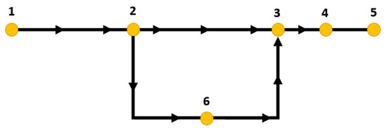
Figure 1.
Simple water network.
For a simple network as shown in Figure 1, the resulting nodal matrix is:
After using the modified reference pressure algorithm on a larger-scale WDS as discussed earlier, the number of locations increases, which is not a cost-effective solution. For an efficient selection of PRV locations, all the PRV candidate locations that appear twice or more than twice during reference pressure variation are selected. Then, each PRV candidate location is selected, and the connectivity of the locations at the downstream end is counted by using nodal matrix analysis.
The function used for counting the number of nodes connected at the downstream node end of the pipeline (PRV candidate locations) is shown in Algorithm 1.
| Algorithm 1: Function for counting the number of nodes connected at the downstream node end of the pipeline |
| function fcnt=count_node(q,M) t_vect=M(q,:); fcnt=0; fcnt=fcnt+sum(t_vect); % fcnt if sum(t_vect)>=1 locs=find(t_vect==1); for i=1:length(locs) fcnt=fcnt+count_node(locs(i),M); end end end |
Note: ‘fcnt’ will store the number of nodes connected to the pipe (represented by q) considering the PRV candidate, and the variable ‘M’ contains the nodal matrix.
Leakage also occurs in joints or nodes due to poor connections. The greater the number of joints or nodes the greater the probability of leakages. The location preferences list is created by arranging the PRV candidate locations in accordance with their number of nodal connections at the downstream end of the pipeline (‘fcnt’ will store the number of nodal connections). The higher the number of nodes connected to the PRV candidate at the downstream end, the better the effect of pressure reduction in the WDS will be. Additionally, more extension of pipes usually means more service connections. Thus, the water losses increase with the extension of the pipeline in the WDS. Thus, the total length of pipes located at the downstream of the PRV candidate pipeline is also considered while creating the preference list of the pipeline. The PRV candidate location with the maximum number of downstream connections and having maximum length of pipeline associated to it appears first in the preference list, and the location with the minimum number of nodal connections and having minimum downstream pipeline length appears last in the preference list. If the PRV candidate pipeline has the same number of nodal connections, then the pipeline with the greater length of pipes located at the downstream is placed higher in the preference list. Depending upon the sanctioned economy, a number of PRV locations is selected from the preference list obtained from the proposed nodal matrix analysis. In this way, using the proposed algorithm, a more effective as well as efficient localization of PRVs will be achieved in the WDS.
2.5. Multi-Objective Genetic Algorithm for PRV Optimization
A multi-objective GA was used for finding the optimized pressure control value across PRVs (Pset) when operating in active mode (adopted from [4,10]). The multi-objective GA includes two objective functions, named as f1 (first) and f2 (second). The first objective (f1) is to determine the optimized operational pressure control value (Pset) of the PRVs. The objective function is defined as:
subject to
where Preq is the desired pressure (in m), which needs to be maintained across all the nodes; nv is the total number of PRVs currently installed in the water network; Pmax and Pmin are the maximum and minimum allowed pressure values across the PRVs; Ns is the total number of nodes in the WDS; Nv is the maximum allowed number of PRVs that can be installed in the WDS; and k is the value of the base demand multiplier (k). Hj,k and Hi,k represent the value of the head at nodes j and i under load condition k. Pset is calculated for the individual load condition k. CL is the coefficient of leakage per unit length; Li is the total length of the pipeline (in m) associated with node i; γ is the leakage exponential used to define relationships between flow from the orifice and pressure. A leakage exponential value of 0.5 was adopted for this study.
Pi,k ≥ Preq
nv ≤ Nv
Hi,j,k = Hi,k − Hj,k
Pmin ≤ Pset ≤ Pmax
The second objective (f2) was utilized to minimize water leakages in the WDS. The objective function is given by [4,10]:
where ( =Li * ) is the flow intensity at node i.
Leakage rate () is determined for every value of Pset for PRVs generated from the (f1). The Pset that belongs to the lowest value of was selected. Pset varies between Pmin and Pmax. The multi-objective GA uses crossover and mutation probabilities of 0.65 and 0.002 for 200 generations, and each generation has a population size of 50.
3. Results and Discussion
Campos Do Conde II Network
The presented technique was applied to a real WDS located in Piracicaba, Brazil, called Campos do Conde II. [23]. This residential water network consists of 124 nodes, 155 pipelines, one PRV (the ID is v154, Pset = 10 m), one reservoir, one tank and one pump, as shown in Figure 2. The details of WDS is given in Table A1 and Table A2. The WDS has total pipeline length of 11,969.83 m. According to Brazilian technical standards, the WDS has a minimal dynamic pressure of 10 m and a maximal static pressure of 50 m [23]. The base demand at each node is given in Table 1. The rest of the nodes, which are not mentioned in the table, do not have any demand. The system has demand variation throughout the day, as shown in Figure 3. The figure shows the demand multiplier (load condition ‘k’) with the base demand for the whole week. The system has an average water consumption of 164.44 LPS. Water demand in the WDS varies from 100.14 L/s (K = 0.609) to 235.14 L/s (k = 1.43).
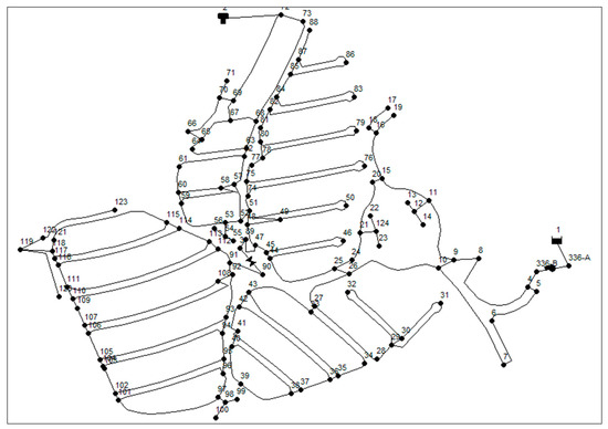
Figure 2.
Campos do Conde II water distribution network [23].

Table 1.
Base demand for various nodes [23].
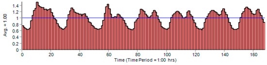
Figure 3.
Demand pattern variation of the water distribution system (WDS) with respect to time [23].
Hydraulic simulations were performed in MATLAB using the EPANET-MATLAB toolkit, and the corresponding commands are discussed in Section 2.1 [21]. PDA analysis was performed using Equation (4). The present study used Pser and Pmi values of 10 and 0 m for all nodes (adopted from [23]). A PRV installed in the WDS has a Pset of 10 m, which may create water deficiency in the WDS as the minimum required pressure is 10 m, and thus the system may not perform in a realistic manner by considering demand-driven analysis only [25]. To overcome such situations if encountered, PDA was performed.
Pressure management is accomplished in the WDS by installing PRVs for leakage control. An optimized number and localization of PRVs can be seen as one of the challenges while opting for PRV-based pressure management in a WDS. An optimized localization of PRVs in the WDS is desired to achieve efficient pressure management, leading to leakage reduction. As mentioned earlier, the pressure value across the WDS changes with respect to time. Determining PRV locations for each load condition (k), which varies from 0.609 to 1.43, is not a feasible option as PRV locations will keep changing with respect to changes in k. Installation of PRVs at all the observed locations for every value of k is a challenging task due to the associated installation costs. Optimal PRV locations were calculated for average load conditions, i.e., a base demand of 164.44 L/s, which is observed at 8:00 AM. Hydraulic simulations of the WDS at 8:00 AM were performed considering average load conditions. Hydraulic parameters, such as the pressure observed during this load condition, were stored. Using these observed pressure values, optimal PRV candidate localizations were identified using Equations (5) and (6). The minimum desired pressure in the WDS is 10 m, whereas 50 m is the maximum allowed pressure [23]. Thus, it is desired that the pressure at each water-demanding node in the WDS should be between 10 and 50 m. Hence, the value of reference pressure varies from 10 to 50 m. After applying the modified reference pressure algorithm (i.e., Equations (5) and (6)) for the given WDS, the value of localization variation with respect to Pref variation is given in Figure 4. The number of PRV locations varies from 28 to 22 after using the modified reference pressure algorithm. The number of PRVs is minimal (i.e., 22) for a Pref of 47 or 50. It is observed that the number of PRVs increases drastically. Moreover, suggested PRV locations also keep changing with respect to the variation in Pref. For example, for a Pref of 47 m, the probable pipeline locations are at pipe no. 3, 5, 27, 97, 47, 143, 58, 34, 62, 35, etc., whereas for a Pref of 50 m, the probable pipeline locations are at pipe no. 3, 5, 27, 97, 47, 4, 58, 152, etc. Thus, there is a possibility that for the selected value of Pref, the system may not be able to find the optimal PRV location. Installation of PRVs in every suggested pipeline (i.e., a total of 22) is not a feasible option. The modified reference pressure algorithm does not tell about the preferences regarding the location of PRVs, i.e., among all the observed probable PRV locations, which pipeline should be preferred first for PRV installation to achieve better pressure management. To overcome this drawback of the modified reference pressure algorithm, the proposed nodal matrix analysis was performed to identify the preferred PRV locations.
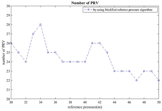
Figure 4.
Number of pressure-reducing valves versus Pref.
Nodal matrix analysis was applied for finding the preferred optimal locations of PRVs among the various PRV candidate locations obtained from the modified reference pressure algorithm. Pipelines that were observed only twice or less than twice as candidate PRV locations during the variation of Pref were eliminated. Such locations will never lead to efficient pressure reduction. This will also reduce the unnecessary calculations. The nodal matrix was created using the steps mentioned in the proposed methodology (Section 2.1). The number of connected nodes or pipelines at the downstream end from all the possible PRV candidates was counted using the count_node function (already mentioned in Section 2.4). Depending upon the number of nodal connections at the downstream end for the selected PRV candidate, the PRV locations were arranged in descending order, as given in Table 2.
Table 2.
Preference list of optimal pressure-reducing valve localizations obtained from the proposed nodal matrix algorithm.
This can be explained by an example in which the PRV reduces the downstream pressure of the node connected to it (let it be Ni). This node is further connected directly or indirectly to other nodes in the WDS (Nj). Thus, a reduction in pressure (Pi) at this node (Ni) will also reduce the pressure (Pj) at the next node (Nj). This will be true for the next node Nz connected to Nj. This means that the higher the number of nodes connected directly or indirectly at the downstream end of the PRV, the greater the pressure reduction at each node, and also that of the whole WDS, will be. Thus, a higher number of nodal connections at the downstream end of the PRV will be more likely to achieve a better pressure reduction, and thus it is placed above in the preference list. Additionally, the total length of pipes located at the downstream of the PRV candidate pipeline was also considered while creating the preference list of pipeline. Table 2 represents the preference list of PRV locations.
It can be identified from Table 2 that for pipeline locations 3, 5, 27, 97, 47, and 150, the number of downstream nodal counts is 117, 108, 70, 15, 14, and 14, respectively. The total length of pipeline at the nodal end for pipeline locations 3, 5, 27, 97, 47, and 150 is 11,516.63, 10,395.38, 8235.9, 1431.43, 752.26, and 706.54 m, respectively. Meanwhile, other locations such as pipes 61, 143, 75, and 58 only have two downstream nodal connections and have a total pipeline length at downstream of 233.6, 215.2, 101.2, and 16.2 m, respectively. Installing PRVs at such locations would not be a feasible solution and would not lead to efficient pressure reduction. This would only increase the infrastructural cost of the WDS. The numbers of connecting nodes are maximal for pipeline locations 3, 5, 27, 97, 150, and 47. Depending upon the economic feasibility of water companies, the first 4–6 locations, i.e., pipes 3, 5, 27, 97, 150, and 47, can be selected for the localization of PRVs. Thus, by providing a preference list of locations of PRV candidates, the proposed algorithm provides an optimal valve localization when compared to the modified reference pressure algorithm [10]. The PRVs in the WDS are installed at pipes 3, 5, 27, and 97.
Another challenge is to maintain the optimized pressure setting across PRVs such that it will reduce the excess pressure in the WDS and will also maintain the minimum required pressure in the WDS for an efficient supply of water. The multi-objective GA was used for finding the Pset of PRVs for every variation under load condition ‘k’ using Equations (8)–(13). The load condition ‘K’ varies from 0.609 to 1.43, i.e., a demand of 100.14 to 235.14 L/s, as given in Figure 2. Pset varies between 10 (Pmin) and 50 m (Pmax). Hydraulic simulations were performed using the EPANET-MATLAB-toolkit. The value of CL is 1.23 × 10⁻⁴ [23]. The operational value of Pset during different load conditions can be identified in Table 3. There is a vast pressure reduction observed after using PRVs at pipes 3, 5, 27, and 97; these optimal PRV candidate locations observed from the proposed nodal matrix analysis lead to efficient pressure management. The pressure difference observed before and after pressure management was calculated. There is an average reduction in surplus pressure of 1380.2 m. The relative leakage reduction was calculated using Equation (3). The relative leakage reduction varies from 15.59% to 30.73% with respect to changes in load condition (k). The adoption of the proposed technique leads to an overall leakage reduction of 20.08%. The infrastructural cost of small-diameter PRVs at pipes 5, 27, and 97 is $67,770 per PRV, and for larger-diameter PRVs, i.e., at pipe 3 is $15,798 [26]. The total infrastructural cost for the placement of the four PRVs in the WDS is $35,889. The addition of a fifth PRV will increase the infrastructural cost of the WDS by approximately $7000 and will only lead to an additional pressure reduction of 0.43%. Leakage reduction will also reduce the water consumption in the WDS, where water was lost earlier. The average energy consumption from the pump is reduced from 1045.58 to 1007 kWh, causing a reduction in the electricity bill by 3%–4%.
Table 3.
The optimal pressure value of the pressure-reducing valve (PRV) (Pset) in meters, obtained after applying the proposed algorithm considering different load conditions.
The adoption of the proposed pressure management technique leads to an overall leakage reduction of 20.08%. The minimum required pressure of 10 m is maintained at every node, which avoids pressure deficiency at the demand node.
4. Conclusions
Pressure-reducing valves are an efficient way of performing pressure management in a water distribution system for leakage control. The modified reference algorithm is a simple technique for identifying pressure-reducing valve locations in water networks. The algorithm fails to find optimal locations of valves in a larger-scale water network as the number of valve candidate locations increases drastically. The presented study proposes a nodal matrix analysis for further improvement of the modified reference pressure algorithm. The algorithm was utilized for the localization of pressure-reducing valves, especially for larger-scale WDSs. The proposed methodology was applied to a real WDS in Piracicaba, Brazil, called Campos do Conde II, for an optimized localization of pressure-reducing valves with an average water consumption of 164.44 L/s. Using the modified reference pressure algorithm, the resulting minimum number of valve candidate locations is 22. Installing such a number of valves is not feasible. Nodal matrix analysis was performed to determine the preferable locations of valves among these observed locations. The preference pressure-reducing valve locations are observed at pipes 3, 5, 27, and 97, which leads to a much lower number than 22. Hence, the proposed model is able to identify a more optimized localization of pressure-reducing valves when compared with the modified reference pressure algorithm. The proposed system shows successful results for larger and real complex water networks. A vast reduction in pressure is observed after using PRVs at pipes 3, 5, 27, and 97; these optimal PRV candidate locations result from the proposed nodal matrix analysis. There is an average reduction in surplus pressure of 1380.2 m. The adoption of the proposed pressure management technique leads to an overall leakage reduction of 20.08%. The infrastructural cost for the placement of four PRVs in the WDS is $35,889. The addition of a fifth PRV will only lead to an additional pressure reduction of 0.43% and will increase the infrastructural cost of the WDS by approximately $7000. Hence, installing a fifth PRV is not a cost-effective solution. The sectorization of the WDS before PRV localization can be investigated in future work. The PRV localization operation can be implemented separately in these sectorized WDSs. This will lead to better PRV localization and will also result in more efficient pressure management.
Author Contributions
Conceptualization, A.G. and N.B.; Methodology, A.G.; Software, A.G.; Validation, A.G., Z.M.Y. and N.B.; Formal Analysis, A.G. and N.B.; Investigation, A.G., N.B. and K.K.; Resources, K.K.; Data Curation, A.G.; Writing—Original Draft Preparation, A.G., N.B. and Z.M.Y.; Writing—Review and Editing, A.G., N.B., Z.M.Y. and K.K.; Visualization, A.G. and Z.M.Y.; Supervision, K.K.; Project Administration, K.K.; Funding Acquisition, N.B. All authors have read and agreed to the published version of the manuscript.
Funding
This research received no external funding.
Acknowledgments
The authors would like to sincerely thank B. Brentan for providing the EPANET input file (.inp) of the Campos do Conde II water distribution network, which has made this analysis possible.
Conflicts of Interest
The authors declare no conflict of interest.
Abbreviations
| EPANET | Environmental Protection Agency Network |
| GA | Genetic algorithm |
| IWA | International Water Association |
| LP | Linear programming |
| LPS | Liters per second |
| MATLAB | Matrix laboratory |
| MINLP | Mixed-integrated nonlinear program |
| NSGA-II | Nondominated sorting genetic algorithm-II |
| PDA | Pressure-driven analysis |
| PRV | Pressure-reducing valve |
| RAM | Random access memory |
| WDS | Water distribution system |
Appendix A. Network Details
Table A1.
Pipeline dimensions of the Campos do Conde II water distribution network, Brazil.
Table A1.
Pipeline dimensions of the Campos do Conde II water distribution network, Brazil.
| Link ID | Start Node | End Node | Length m | Diameter mm |
| 115 | 115 | 121 | 230.79 | 50 |
| 114 | 114 | 115 | 24.25 | 100 |
| 113 | 113 | 114 | 58.74 | 100 |
| 112 | 112 | 113 | 20.56 | 100 |
| 111 | 91 | 112 | 36.26 | 100 |
| 110 | 90 | 91 | 19.98 | 150 |
| 108 | 47 | 89 | 33.23 | 150 |
| 107 | 40 | 38 | 145.99 | 50 |
| 106 | 37 | 41 | 163.09 | 50 |
| 105 | 42 | 36 | 213.63 | 50 |
| 104 | 43 | 42 | 12.25 | 100 |
| 103 | 41 | 42 | 57.38 | 50 |
| 102 | 40 | 41 | 20.39 | 50 |
| 101 | 39 | 40 | 75.82 | 50 |
| 100 | 38 | 39 | 101.1 | 50 |
| 99 | 37 | 38 | 18.3 | 50 |
| 98 | 36 | 37 | 55.4 | 50 |
| 97 | 35 | 36 | 16.84 | 50 |
| 96 | 43 | 33 | 141.31 | 100 |
| 95 | 35 | 43 | 220.72 | 50 |
| 94 | 34 | 35 | 53.31 | 50 |
| 93 | 33 | 34 | 135.9 | 50 |
| 92 | 27 | 33 | 12.25 | 100 |
| 91 | 29 | 30 | 11.24 | 50 |
| 90 | 32 | 29 | 132.51 | 50 |
| 89 | 30 | 32 | 134.67 | 50 |
| 88 | 31 | 30 | 98.04 | 50 |
| 87 | 29 | 31 | 120.57 | 50 |
| 86 | 28 | 29 | 48.74 | 50 |
| 85 | 27 | 28 | 148.73 | 100 |
| 84 | 26 | 27 | 104.82 | 100 |
| 83 | 68 | 73 | 200.65 | 50 |
| 82 | 72 | 73 | 40.89 | 50 |
| 81 | 69 | 72 | 186.62 | 50 |
| 80 | 70 | 71 | 12.22 | 50 |
| 79 | 70 | 69 | 12 | |
| Link ID | Start Node | End Node | Length m | Diameter mm |
| 78 | 66 | 70 | 99.22 | 50 |
| 77 | 65 | 66 | 12.25 | 50 |
| 76 | 67 | 69 | 30.99 | 50 |
| 75 | 68 | 67 | 47.49 | 50 |
| 74 | 63 | 68 | 53.08 | 100 |
| 73 | 65 | 67 | 85.4 | 50 |
| 72 | 64 | 65 | 6.89 | 50 |
| 71 | 63 | 64 | 102.91 | 50 |
| 70 | 62 | 63 | 14.67 | 100 |
| 69 | 57 | 62 | 51.55 | 100 |
| 68 | 61 | 62 | 122.4 | 50 |
| 67 | 60 | 61 | 45.82 | 50 |
| 66 | 59 | 60 | 13.2 | 50 |
| 65 | 58 | 60 | 105.01 | 50 |
| 64 | 57 | 58 | 6.8 | 50 |
| 63 | 52 | 57 | 64.75 | 100 |
| 62 | 59 | 58 | 117.66 | 50 |
| 61 | 53 | 59 | 115.34 | 50 |
| 60 | 54 | 56 | 7.93 | 50 |
| 59 | 54 | 55 | 8.4 | 50 |
| 58 | 53 | 54 | 11.32 | 50 |
| 57 | 52 | 53 | 28.06 | 50 |
| 56 | 87 | 88 | 63.44 | 50 |
| 55 | 85 | 87 | 23.1 | 50 |
| 54 | 86 | 87 | 103.76 | 50 |
| 53 | 85 | 86 | 104.66 | 50 |
| 52 | 84 | 85 | 58.8 | 50 |
| 51 | 82 | 84 | 23.29 | 50 |
| 50 | 83 | 84 | 155 | 50 |
| 49 | 82 | 83 | 162.76 | 50 |
| 48 | 81 | 82 | 5.58 | 100 |
| 47 | 80 | 81 | 51.87 | 100 |
| 46 | 78 | 80 | 18.22 | 100 |
| 45 | 79 | 80 | 193.53 | 50 |
| 44 | 78 | 79 | 194.76 | 50 |
| 43 | 77 | 78 | 5.37 | 100 |
| 42 | 75 | 77 | 47.33 | 100 |
| Link ID | Start Node | End Node | Length m | Diameter mm |
| 41 | 74 | 75 | 14.13 | 100 |
| 40 | 76 | 75 | 222.78 | 50 |
| 39 | 74 | 76 | 221.69 | 50 |
| 38 | 51 | 74 | 55.58 | 100 |
| 37 | 51 | 52 | 11 | 100 |
| 36 | 48 | 51 | 8.12 | 150 |
| 35 | 50 | 49 | 197.48 | 50 |
| 34 | 49 | 50 | 178.2 | 50 |
| 33 | 48 | 49 | 6.54 | 50 |
| 32 | 47 | 48 | 41.54 | 150 |
| 31 | 45 | 47 | 24.55 | 150 |
| 30 | 44 | 45 | 13.06 | 150 |
| 29 | 46 | 45 | 144.92 | 50 |
| 28 | 44 | 46 | 141.26 | 50 |
| 27 | 25 | 44 | 164.85 | 150 |
| 26 | 26 | 25 | 17.64 | 150 |
| 25 | 24 | 25 | 13.73 | 50 |
| 24 | 21 | 24 | 53.25 | 50 |
| 23 | 124 | 23 | 6.08 | 50 |
| 22 | 124 | 22 | 5.76 | 50 |
| 21 | 21 | 124 | 10.69 | 50 |
| 20 | 20 | 21 | 97.21 | 50 |
| 19 | 15 | 20 | 17.62 | 50 |
| 18 | 10 | 26 | 172.76 | 200 |
| 17 | 18 | 17 | 51.4 | 50 |
| 16 | 16 | 18 | 16.77 | 50 |
| 15 | 16 | 19 | 45.19 | 50 |
| 14 | 15 | 16 | 84.9 | 50 |
| 13 | 11 | 15 | 97.97 | 50 |
| 12 | 12 | 13 | 5.91 | 50 |
| 11 | 12 | 14 | 5.54 | 50 |
| 10 | 11 | 12 | 12.09 | 50 |
| 9 | 9 | 11 | 120.11 | 50 |
| 8 | 9 | 10 | 16.41 | 200 |
| 7 | 10 | 7 | 210.5 | 50 |
| 6 | 8 | 9 | 5.94 | 200 |
| 5 | 4 | 8 | 186.24 | 200 |
| 4 | 6 | 7 | 95.47 | 50 |
| Link ID | Start Node | End Node | Length m | Diameter mm |
| 3 | 5 | 6 | 103.2 | 50 |
| 2 | 4 | 5 | 17.72 | 50 |
| 153 | 117 | 115 | 218.09 | 50 |
| 152 | 114 | 116 | 229.97 | 50 |
| 151 | 111 | 113 | 269.14 | 50 |
| 150 | 112 | 110 | 278.96 | 50 |
| 149 | 92 | 108 | 12.59 | 100 |
| 148 | 107 | 108 | 266.52 | 50 |
| 147 | 106 | 108 | 278.4 | 50 |
| 146 | 105 | 93 | 238.55 | 50 |
| 145 | 94 | 104 | 228.07 | 50 |
| 144 | 95 | 102 | 204.81 | 50 |
| 143 | 96 | 101 | 200.57 | 50 |
| 142 | 94 | 95 | 50.58 | 100 |
| 141 | 93 | 94 | 19.73 | 100 |
| 140 | 92 | 93 | 80.46 | 100 |
| 139 | 91 | 92 | 23.79 | 100 |
| 138 | 96 | 95 | 14.74 | 50 |
| 137 | 97 | 96 | 57.47 | 50 |
| 136 | 98 | 100 | 12.95 | 50 |
| 135 | 98 | 99 | 15.12 | 50 |
| 134 | 97 | 98 | 11.43 | 50 |
| 133 | 101 | 97 | 210.89 | 50 |
| 132 | 102 | 101 | 13.29 | 50 |
| 131 | 103 | 102 | 48.53 | 50 |
| 130 | 104 | 103 | 4.31 | 50 |
| 129 | 105 | 104 | 14.11 | 50 |
| 128 | 106 | 105 | 51.81 | 50 |
| 127 | 107 | 106 | 15.62 | 50 |
| 126 | 109 | 107 | 45.73 | 50 |
| 125 | 110 | 109 | 6.78 | 50 |
| 124 | 111 | 110 | 14.52 | 50 |
| 123 | 116 | 111 | 50.86 | 50 |
| 122 | 117 | 116 | 17.26 | 50 |
| 121 | 118 | 117 | 10.56 | 50 |
| 120 | 119 | 120 | 85.28 | 50 |
| 119 | 122 | 123 | 151.41 | 50 |
| 118 | 119 | 122 | 9.91 | 50 |
| 117 | 118 | 119 | 12.25 | 50 |
| Link ID | Start Node | End Node | Length m | Diameter mm |
| 116 | 121 | 118 | 13.31 | 50 |
| P-1 | 1 | 336-A | 14.17 | 200 |
| P-2 | 336-B | 4 | 6.70649 | 200 |
| 1 | 72 | 2 | 50 | 100 |
| 109 | 89 | 3 | 12.98 | 150 |
| 160 | 336-A | 336-B | #N/A | Pump |
Note: The roughness coefficient for the entire pipe is 0.00015 mm. The diameter of valve 154 connected between nodes 90 and 3 is 150 mm. The tank is connected to node 2 through link 1. The tank has an elevation of 605 m and diameter of 15 m, with a maximum water storage height of 20 m. The tank has initial level of 8 m. The pump has a pump curve equation, given as Head = 33.333 − 0.0068*(flow2).
Table A2.
Details of nodes and their elevation Campos do Conde II water distribution network, Brazil.
Table A2.
Details of nodes and their elevation Campos do Conde II water distribution network, Brazil.
| Node ID | Elevation (m) | Node ID | Elevation (m) | Node ID | Elevation (m) |
|---|---|---|---|---|---|
| Junc 124 | 615.3 | Junc 44 | 603.3 | Junc 57 | 603.3 |
| Junc 123 | 584.5 | Junc 43 | 602.9 | Junc 56 | 601.8 |
| Junc 122 | 575.205 | Junc 42 | 602.3 | Junc 55 | 603 |
| Junc 121 | 575.6 | Junc 41 | 599.9 | Junc 54 | 602.4 |
| Junc 120 | 577.2 | Junc 40 | 599.3 | Junc 53 | 602.4 |
| Junc 119 | 574.5 | Junc 39 | 598.113 | Junc 52 | 604.3 |
| Junc 118 | 575.9 | Junc 38 | 599.3 | Junc 51 | 604.8 |
| Junc 117 | 576 | Junc 37 | 600 | Junc 45 | 603.2 |
| Junc 116 | 576.8 | Junc 36 | 603.218 | Junc 69 | 598.6 |
| Junc 115 | 593.5 | Junc 35 | 603.8 | Junc 68 | 604.3 |
| Junc 114 | 595.6 | Junc 34 | 605.9 | Junc 67 | 599.3 |
| Junc 113 | 599.9 | Junc 33 | 608.3 | Junc 50 | 616.2 |
| Junc 112 | 601.2 | Junc 32 | 612 | Junc 49 | 605.2 |
| Junc 111 | 578.4 | Junc 31 | 616.83 | Junc 48 | 605 |
| Junc 110 | 578.8 | Junc 30 | 610.1 | Junc 47 | 605.3 |
| Junc 109 | 579 | Junc 29 | 609.4 | Junc 46 | 614.2 |
| Junc 108 | 601.6 | Junc 28 | 606.6 | Junc 74 | 604.5 |
| Junc 107 | 580.1 | Junc 27 | 608.069 | Junc 73 | 610 |
| Junc 106 | 580.2 | Junc 26 | 612.9 | Junc 72 | 603.321 |
| Junc 105 | 580.6 | Junc 25 | 612.9 | Junc 71 | 598 |
| Junc 104 | 581 | Junc 24 | 613.8 | Junc 70 | 597.4 |
| Junc 103 | 581 | Junc 23 | 615.1 | Junc 62 | 603 |
| Junc 102 | 581 | Junc 22 | 615.5 | Junc 61 | 591.2 |
| Junc 101 | 581 | Junc 21 | 615.9 | Junc 60 | 593.3 |
| Junc 100 | 593.7 | Junc 20 | 619.3 | Junc 59 | 595.1 |
| Junc 99 | 595.8 | Junc 19 | 624 | Junc 58 | 602.8 |
| Junc 98 | 594.7 | Junc 18 | 620.3 | Junc 79 | 618.7 |
| Junc 97 | 595.012 | Junc 17 | 623.5 | Junc 78 | 604.3 |
| Junc 96 | 597.4 | Junc 16 | 620.6 | Junc 77 | 604.2 |
| Junc 95 | 597.8 | Junc 15 | 620.2 | Junc 76 | 618.655 |
| Junc 94 | 598.646 | Junc 14 | 621.9 | Junc 75 | 604.3 |
| Junc 93 | 600 | Junc 13 | 621.8 | Tank 2 | 605 |
| Junc 92 | 602.2 | Junc 12 | 621.8 | Junc 66 | 591.3 |
| Junc 91 | 602.3 | Junc 11 | 622.4 | Junc 65 | 592.9 |
| Junc 90 | 603.4 | Junc 10 | 620 | Junc 64 | 592.324 |
| Junc 89 | 604.2 | Junc 9 | 620.4 | Junc 63 | 603 |
| Junc 88 | 612.1 | Junc 8 | 620.4 | Junc 82 | 606.1 |
| Junc 87 | 609.568 | Junc 7 | 614.7 | Junc 81 | 605.8 |
| Junc 86 | 618.5 | Junc 6 | 617.3 | Junc 80 | 604.5 |
| Junc 85 | 609.6 | Junc 5 | 626.69 | Junc 336-B | 627.7544222 |
| Junc 84 | 607 | Junc 4 | 626.69 | Junc 3 | 603.4 |
| Junc 83 | 619 | Junc 336-A | 614 | Resvr 1 | 625 |
References
- Gleick, P.H. Global water resources: The coming crises. In Human Impact on the Environment; Routledge: London, UK, 2019; pp. 161–170. [Google Scholar]
- Gao, J.; Li, C.; Zhao, P.; Zhang, H.; Mao, G.; Wang, Y. Insights into water-energy cobenefits and trade-offs in water resource management. J. Clean. Prod. 2019, 213, 1188–1203. [Google Scholar] [CrossRef]
- Lambert, A. What do we know about pressure-leakage relationships in distribution systems. In Proceedings of the IWA System Approach to Leakage Control and Water Distribution Systems Management, Brno, Czech Republic, 16–18 May 2001. [Google Scholar]
- Gupta, A.; Mishra, S.; Bokde, N.; Kulat, K. Need of smart water systems in India. Int. J. Appl. Eng. Res. 2016, 11, 2216–2223. [Google Scholar]
- Grace, S.R.P.; Stephen, P.; Paul, J.J.; Thusnavis, B.M.I. A Review on the Monitoring and localization of leakage in water distribution system. In Proceedings of the 2019 2nd International Conference on Signal Processing and Communication (ICSPC), Coimbatore, India, 29–30 March 2019; pp. 83–88. [Google Scholar]
- Hatam, F.; Blokker, M.; Besner, M.-C.; Ebacher, G.; Prévost, M. Using Nodal Infection Risks to Guide Interventions Following Accidental Intrusion due to Sustained Low Pressure Events in a Drinking Water Distribution System. Water 2019, 11, 1372. [Google Scholar] [CrossRef]
- Vicente, D.J.; Garrote, L.; Sánchez, R.; Santillán, D. Pressure Management in Water Distribution Systems: Current Status, Proposals, and Future Trends. J. Water Resour. Plan. Manag. 2016, 142, 4015061. [Google Scholar] [CrossRef]
- Araujo, L.S.; Ramos, H.; Coelho, S.T. Pressure Control for Leakage Minimisation in Water Distribution Systems Management. Water Resour. Manag. 2006, 20, 133–149. [Google Scholar] [CrossRef]
- Dai, P.D.; Li, P. Optimal Localization of Pressure Reducing Valves in Water Distribution Systems by a Reformulation Approach. Water Resour. Manag. 2014, 28, 3057–3074. [Google Scholar] [CrossRef]
- Gupta, A.D.; Bokde, N.; Marathe, D.; Kulat, K. Optimization techniques for leakage management in urban water distribution networks. Water Sci. Technol. Water Supply 2017, 17, 1638–1652. [Google Scholar] [CrossRef]
- Bhagat, S.K.; Welde, W.; Tesfaye, O.; Tung, T.M.; Al-Ansari, N.; Salih, S.Q.; Yaseen, Z.M. Evaluating physical and fiscal water leakage in water distribution system. Water 2019, 11, 2091. [Google Scholar] [CrossRef]
- García, J.M.; Salcedo, C.; Saldarriaga, J. Minimization of Water Losses in WDS through the Optimal Location of Valves and Turbines: A Comparison between Methodologies. In World Environmental and Water Resources Congress 2019: Hydraulics, Waterways, and Water Distribution Systems Analysis; American Society of Civil Engineers: Reston, VA, USA, 2019; pp. 437–445. [Google Scholar]
- Güngör, M.; Yarar, U.; Cantürk, Ü.; Fırat, M. Increasing Performance of Water Distribution Network by Using Pressure Management and Database Integration. J. Pipeline Syst. Eng. Pract. 2019, 10, 4019003. [Google Scholar] [CrossRef]
- Jowitt, P.W.; Xu, C. Optimal Valve Control in Water-Distribution Networks. J. Water Resour. Plan. Manag. 1990, 116, 455–472. [Google Scholar] [CrossRef]
- Gupta, A.; Bokde, N.; Kulat, K.D. Hybrid Leakage Management for Water Network Using PSF Algorithm and Soft Computing Techniques. Water Resour. Manag. 2017, 32, 1133–1151. [Google Scholar] [CrossRef]
- Reis, L.F.R.; Porto, R.M.; Chaudhry, F.H. Optimal Location of Control Valves in Pipe Networks by Genetic Algorithm. J. Water Resour. Plan. Manag. 1997, 123, 317–326. [Google Scholar] [CrossRef]
- Creaco, E.; Pezzinga, G. Multiobjective Optimization of Pipe Replacements and Control Valve Installations for Leakage Attenuation in Water Distribution Networks. J. Water Resour. Plan. Manag. 2015, 141, 4014059. [Google Scholar] [CrossRef]
- Nicolini, M.; Zovatto, L. Optimal Location and Control of Pressure Reducing Valves in Water Networks. J. Water Resour. Plan. Manag. 2009, 135, 178–187. [Google Scholar] [CrossRef]
- Dai, P.D.; Li, P. Optimal Pressure Regulation in Water Distribution Systems Based on an Extended Model for Pressure Reducing Valves. Water Resour. Manag. 2016, 30, 1239–1254. [Google Scholar] [CrossRef]
- Liberatore, S.; Sechi, G.M. Location and Calibration of Valves in Water Distribution Networks Using a Scatter-Search Meta-heuristic Approach. Water Resour. Manag. 2008, 23, 1479–1495. [Google Scholar] [CrossRef]
- Eliades, D.G.; Kyriakou, M.; Vrachimis, S.; Polycarpou, M.M. EPANET-MATLAB toolkit: An open-source software for interfacing EPANET with MATLAB. In Proceedings of the 14th International Conference on Computing and Control for the Water Industry (CCWI), Amsterdam, The Netherlands, 7–9 November 2016. [Google Scholar]
- Shang, F.; Uber, J.G.; Rossman, L.A.; Janke, R. EPANET Multi-Species Extension User’s Manual; Risk Reduction Engineering Laboratory, US Environmental Protection Agency: Cincinnati, OH, USA, 2008.
- Brentan, B.M.; Luvizotto, E.; Montalvo, I.; Izquierdo, J.; Pérez-García, R. Near Real Time Pump Optimization and Pressure Management. Procedia Eng. 2017, 186, 666–675. [Google Scholar] [CrossRef]
- Giustolisi, O.; Savic, D.; Kapelan, Z. Pressure-Driven Demand and Leakage Simulation for Water Distribution Networks. J. Hydraul. Eng. 2008, 134, 626–635. [Google Scholar] [CrossRef]
- Adedeji, K.B.; Hamam, Y.; Abu-Mahfouz, A.M. Impact of Pressure-Driven Demand on Background Leakage Estimation in Water Supply Networks. Water 2019, 11, 1600. [Google Scholar] [CrossRef]
- Creaco, E.; Walski, T. Economic Analysis of Pressure Control for Leakage and Pipe Burst Reduction. J. Water Resour. Plan. Manag. 2017, 143, 4017074. [Google Scholar] [CrossRef]
© 2020 by the authors. Licensee MDPI, Basel, Switzerland. This article is an open access article distributed under the terms and conditions of the Creative Commons Attribution (CC BY) license (http://creativecommons.org/licenses/by/4.0/).