Proposal for a Method Predicting Suitable Areas for Installation of Ground-Source Heat Pump Systems Based on Response Surface Methodology

Abstract

The installation potential of ground-source heat pump (GSHP) systems has been studied based on the spatial interpolation of numerical simulation results using ground heat exchanger (GHE) models. This study is the first to create an estimation formula for the heat exchange rate (HER) to obtain a solution equivalent to the numerical analysis results considering the average method when supplying three-dimensional (3D) hydrogeological information that affects the HER to a two-dimensional (2D) map. It was found that the main factors affecting the HER were groundwater flow velocity, subsurface temperature, and thermal conductivity. The response surface methodology was utilized to approximate the HER using the above-mentioned three parameters. The estimated HER showed very strong agreement with that calculated by the GHE models. The application of the estimation formula to the simulation of the 3D groundwater flow and heat transport model of the Sendai Plain (Japan) better reflects the hydrogeological information of the regional model than conventional maps. The proposed method improves the spatial resolution of maps and allows for the easy creation of the HER estimation formula.

1. Introduction

Ground source heat pump (GSHP) systems are an energy-efficient and environment-friendly technology [1,2,3,4]. They use the natural thermal energy of the subsurface stored at shallow depths for space heating/cooling and snow-melting, among other uses [5,6,7]. It is reported that the efficiency of thermal exchange of the closed loop system depends on thermal conductivity, heat capacity, and subsurface temperature profile [8]. Sensitivity analysis also showed the results that both the design parameters and operational parameters have a major influence on the GSHP performance [9]. The influence of unsaturated condition and groundwater flow on the performance of GSHPs was examined, which showed that groundwater level affected the performance of the GSHP system [10]. Therefore, it is important to subsurface conditions. In Europe, the “Cheap-GSHPs” (Cheap and efficient application of reliable Ground Source Heat exchangers and Pumps) European project has developed a Decision Support System to assist the decision-making process of GSHP system designers and building owners [11].

In Japan, GSHP suitability mapping has been carried out for increasing the number of installations of GSHP systems. The installation potential of GSHP systems was investigated using field survey data [12] and numerical simulation [1,13,14]. Many studies showed that groundwater flow velocity increases the heat exchange rate (HER) and temperature distribution in the vicinity of the ground heat exchanger (GHE) [10,15,16,17,18,19]. The development and uptake of this system in Japan are gradually increasing. However, the number of installations of closed-loop GSHP systems in Japan is about 2700 as of March 2018 [20], which is lower than at other locations around the world, such as Europe and America. This is mainly because it is expensive to install such systems, and GSHP systems are not recognized in Japan. While policies on the introduction of renewable energies are being implemented in each municipality, GSHP systems have not been positioned as an environmental policy in many municipalities. It is also a problem that the public does not have the opportunity to know the GSHP systems. As one of the ways of solving this, suitability maps for the systems are created for each municipality or basin and plain in Japan. This map allows you to grasp the area of a region with relatively high potential for the GSHP systems, and it is expected that local governments and residents will be able to start and help when considering where to introduce the systems. In addition, it is also expected that publishing the map will lead the public to recognize the systems. This potential represents the result of HER under certain operating conditions of a GSHP system, and the method of evaluating this potential is as follows: first, a regional groundwater flow and heat transport simulation is performed. Next, the locations where the GHE model is created are selected in the area where the potential map is to be created, and the HER is calculated by inputting the simulation results and input parameters extracted from the regional model to each constructed GHE model. Finally, the potential map is created by spatially complementing the results of the GHE model. However, numerical simulation of the installation potential was done based on spatial interpolation of the HER in a geographic information system (GIS), and suitability maps for GSHP systems were created without fully reflecting the results of the numerical simulation. Increasing the number of pilot points increases the resolution of the potential map; however, it also increases the time needed to create the map, which is the challenge addressed in this study.

Here, a new method of evaluating the suitability of GSHP systems was proposed to reflect the hydrogeological conditions on the suitability map. Specifically, based on the numerical simulations which were conducted by Kaneko et al. [21], an optimization technique was developed and applied to the model area in this study. Kaneko et al. [21] constructed a regional groundwater flow and heat transport model, and heat exchange simulations have been conducted for each GHE model at the pilot points (GHE locations). We apply the mathematical optimization method to the numerical simulation results of the GHE locations to approximate the HER based on the numerical simulation results of the regional model. As a result, it is possible to create a map of the HER using the result of each mesh of the regional model with data on hydrogeological conditions. When creating a potential map using an optimization method, it is necessary to examine the average in the depth direction to transfer 3D hydrogeological data onto a 2D map, because this method uses average hydrogeological parameters. In this study, the hydrogeological parameters affecting the HER were first examined in terms of the average in vertical direction, which is the novelty of this study. Then, an estimation formula for the HER was created via the optimization method using the relationship between the HER calculated by the GHE models created by Kaneko et al. [21] and the hydrogeological parameters of the GHE models. These parameters were also extracted from the central coordinates of the regional model created by Kaneko et al. [21], and the estimation formula was applied to the extracted parameters to obtain a HER in the study area. The proposed suitable evaluation method, which combines numerical simulation and mathematical optimization methods, is unique to this study. Additionally, this method can be evaluated with higher accuracy and in a shorter time than before, which can be effective to select suitable locations for GSHP system installations and promote the growth of such systems in Japan.

2. Review of Hydrogeological Information and Numerical Simulation of the Study Area

The study area is the Sendai Plain, which is located in Miyagi Prefecture. The plain stretches in the N–S and W–E direction with a distance of 40 km and 10 km, respectively (Figure 1). Small-scale alluvial fans are observed in the inland area, and low-lying shore and dunes exist in the seacoast area of the plain. The Quaternary is composed of clay, sand, and gravel layers, and the Neogene is mainly composed of mudstone. The 3D groundwater flow and heat transport model (regional model) were constructed using the finite element software FEFLOW [22] to evaluate the suitability of the GSHP system by Kaneko et al. [21]. In the software, the calculation of the temperature distribution in the GHE is based on Al-Khoury et al. [16] and Al-Khoury and Bonnier [17]. The size of the modeled area was about 3600 km², considering the catchment area of the plain (Figure 2). The horizontal mesh of the model was refined along the rivers and major areas of the plain. In the vertical direction, layers 1–2, layers 3–9 and layers 10–17 belong to the Quaternary system, the upper Neogene and the lower Neogene, respectively. Steady-state simulation was conducted in the analysis, and this constructed model was validated by comparing the calculated values of hydraulic heads, subsurface temperature profiles (vertical distribution of subsurface temperature), and thermal response test (TRT) with their corresponding measured field data in the plain [21]. Hydraulic heads and subsurface temperature profiles were obtained by groundwater monitoring wells.

Table 1. Input parameters of the regional model of the Sendai Plain quoted from Kaneko et al. [21].

Layer	Formation (Thickness of the Formation (m))	Horizontal Hydraulic Conductivity (m/Day)	Vertical Hydraulic Conductivity (m/Day)	Porosity (−)	Thermal Conductivity of Solids (W/m/K)
1–2	Quaternary (<80 m)	5.0	2.5	0.2	1.4
3–9	Upper Neogene (540–620 m)	0.4	0.2	0.1	1.5
10–17	Lower Neogene (300 m)	0.08	0.04	0.1	1.8

shows the hydrogeological and physical parameters of the model. Input parameters to the model were determined by trial and error by comparing calculated and measured values by Kaneko et al. [21].

Heat exchange simulations were conducted for space heating for each GHE model at the respective locations by Kaneko et al. [21] using FEFLOW [22]. Identical 20 m × 20 m × 120 m GHE models were constructed at 33 locations in the Sendai Plain, assuming a general closed-loop system (Figure 3). Parameters input to the GHE models are the same as those assigned for the analysis model, as shown in Table 1. The same hydrogeological parameters from the same GHE locations in the regional model were assigned for each GHE model. Similarly, initial and boundary conditions of the GHE models were set based on the groundwater flow velocity, hydraulic head, and underground temperature calculated from the analysis model at each GHE location. A GHE was set at a depth of 100 m at the central nodes of the GHE models. A double U-tube with a diameter of 34 mm and silica sand grout were considered. The HER was calculated at each GHE location based on the following conditions: an operating scenario of 120 d of space heating per year from December to March, assuming 24-h operation; inlet temperature and flow rate of the circulation fluid at 5 °C and 20 L/min, respectively. In this paper, the operating scenario of the GSHP system is calculated by the above condition. This study was performed based on a regional model which has been calibrated, and the GHE models in the Sendai Plain (Japan) by Kaneko et al. [21]. The reginal model was verified by 1 TRT, 9 groundwater levels, and 11 subsurface temperature profiles.

3. Study Methods

3.1. Response Surface Methodology

Figure 4 shows a flowchart of the proposed method in this paper. In this study, the hydrogeological condition input to the GHE model and the simulation result of the model were extracted, and the factors affecting HER were statistically analyzed. In the GHE model, hydrogeological parameters include horizontal/vertical hydraulic conductivity, specific storage, thermal conductivity of solid and fluid, volumetric heat capacity, and porosity. The simulation results also include hydraulic heat, subsurface temperature, and groundwater flow velocity. These parameters were average values from the surface to 100 m depth in the analysis because the length of the GHE was set to 100 m. As a result, the HER was correlated with groundwater flow velocity, $v$, subsurface temperature, $T$, and, thermal conductivity of the solid, ${\lambda }_s$. It was judged that the HER can be expressed as the function which uses the above three variables. The response surface methodology (RSM) was utilized as a mathematical optimization method, which was used to approximate the HER by Tomigashi et al. [23], consisting of the above three variables in this study. When a quadratic polynomial is used as the response function, the response surface is expressed by the following equation:

$${y=\beta }_0+{\displaystyle \sum }_{i=1}^n{\beta }_i{x}_i+{\displaystyle \sum }_{i=1}^n{\beta }_{ii}{x}_i^2+{\displaystyle \sum }_{i<j}^n{\beta }_{ij}{x}_i{x}_j$$

(1)

where, ${\beta }_0$,${\beta }_i$, ${\beta }_{ii}$, and ${\beta }_{ij}$ are the regression coefficients and the x values are the variables. When the HER Q is approximated by the three variables, Equation (1) is expressed by the following biquadratic polynomial:

$$Q\cong {\beta }_0{+\beta }_1{v+\beta }_2{T+\beta }_3{\lambda }_s{+\beta }_4{v}^2{+\beta }_5{T}^2{+\beta }_6{\lambda }_s^2{+\beta }_7{vT+\beta }_8{v\lambda }_s{+\beta }_9{T\lambda }_s$$

(2)

where ${\beta }_1$ to ${\beta }_9$ are regression coefficients, $v$ is the groundwater flow velocity, $T$ is the subsurface temperature, and ${\lambda }_s$ is the thermal conductivity of solids, respectively. In this method, it is necessary to average the three parameters that change in the depth direction because the parameters input to the GHE model are not uniform values but values that can change in the depth direction. It is also reported by Vu-Bac et al. [24] that surrogate models such as polynomial regression models have to be utilized as alternative models based on which the sensitivity indices are estimated. In this study, the GHE model was created, and the averaging in the depth direction was examined before estimating the heat exchange amount using Equation (2) in the next section. This examination used the finite element software FEFLOW [22].

3.2. Examination of the Average Method

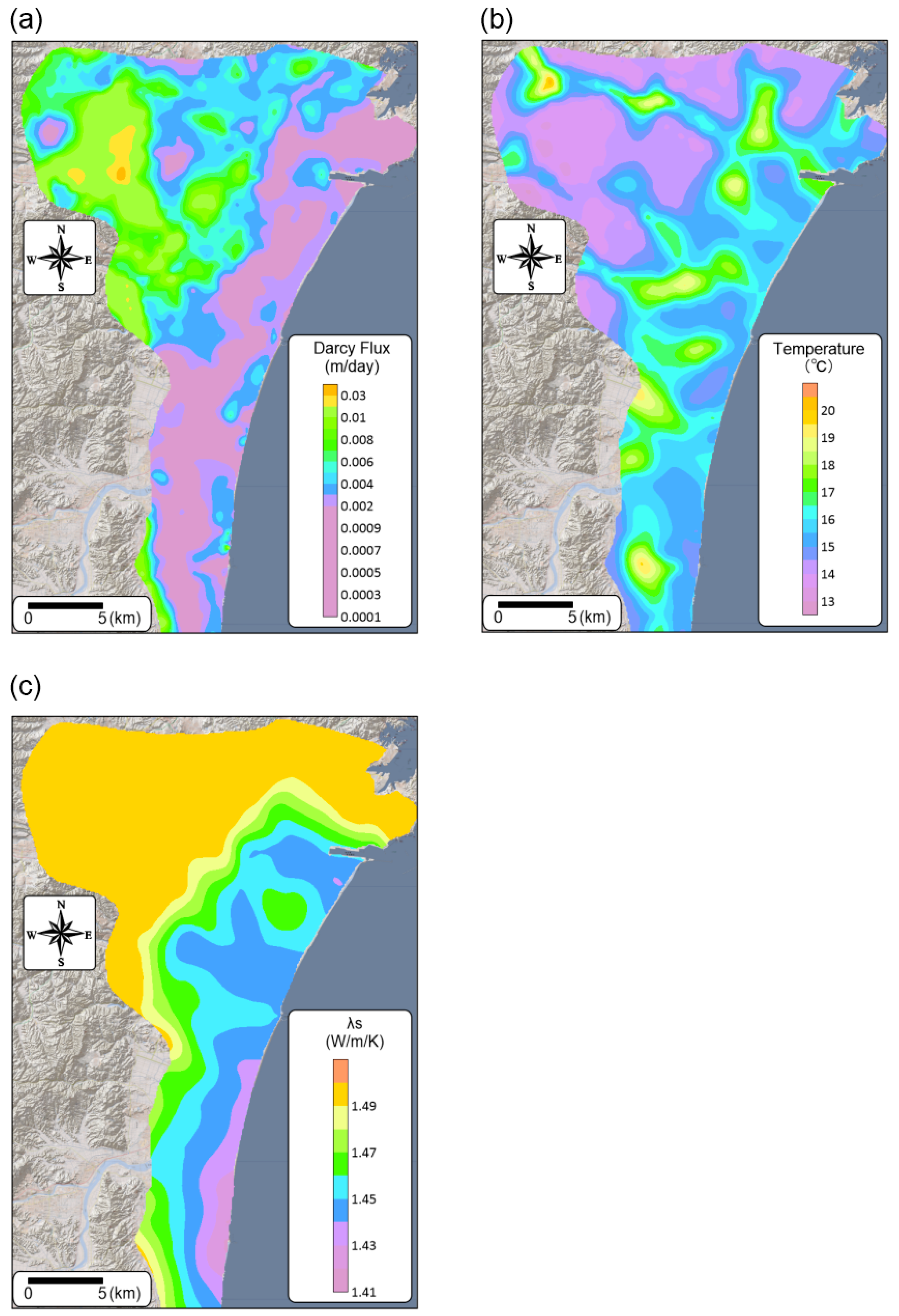
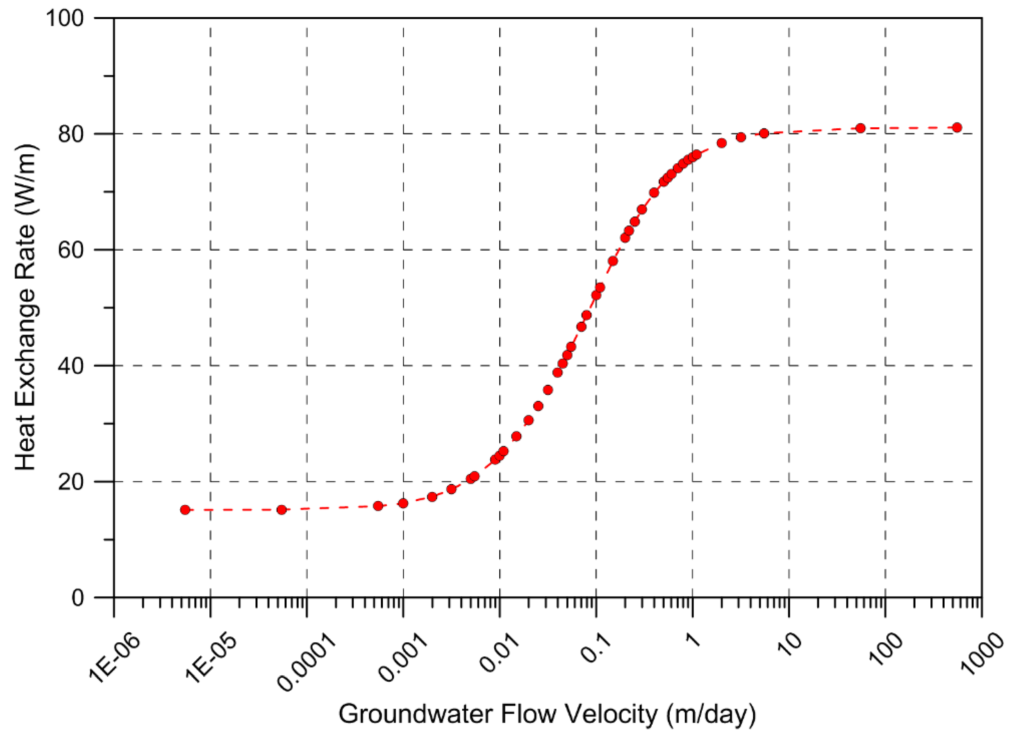
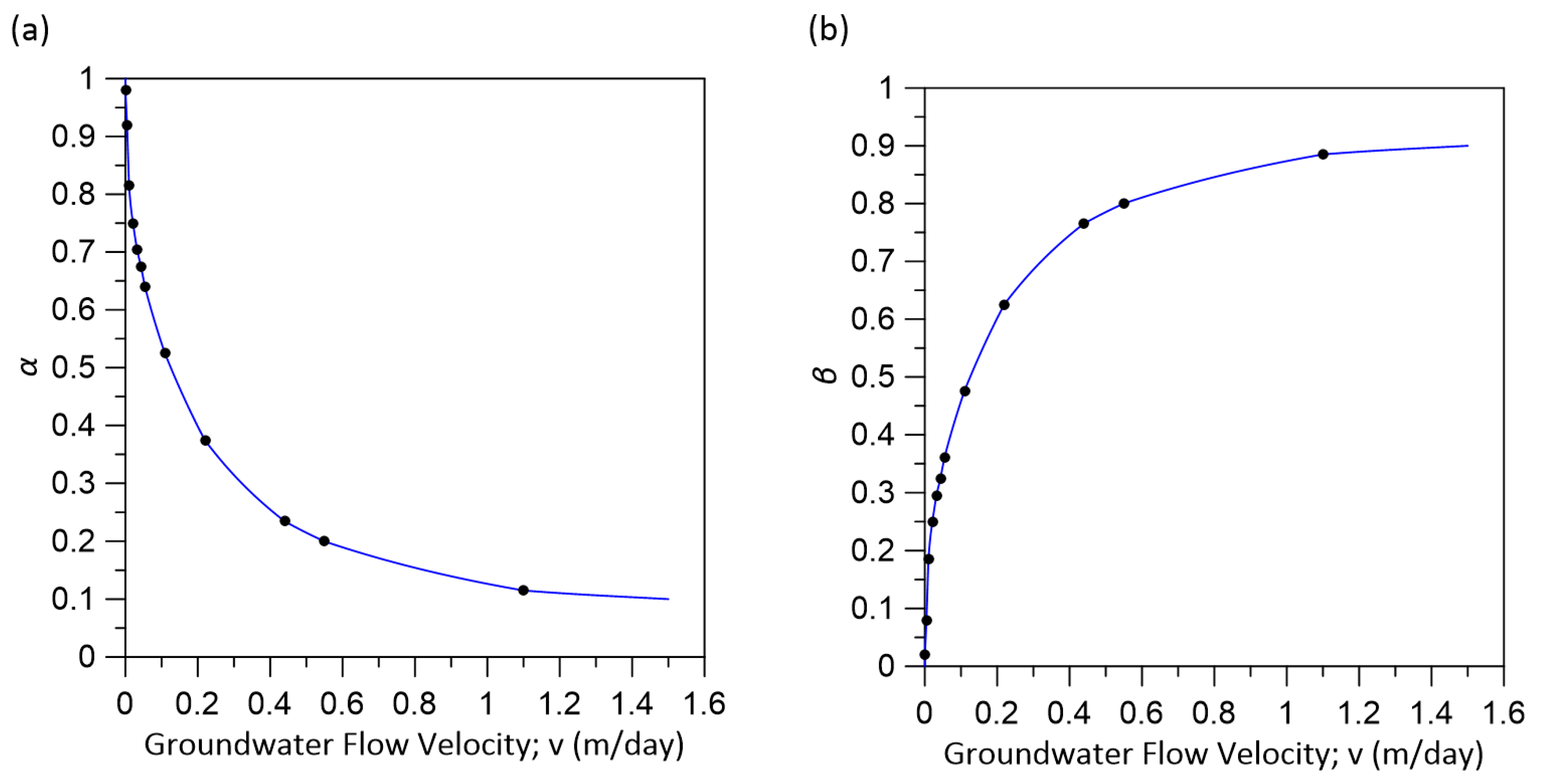
3.2.1. Groundwater Flow Velocity

The averaging of groundwater flow velocity was examined. The formations in the study area are mainly from the Quaternary and Neogene from the surface to a depth of 100 m, which were input to the regional model of the Sendai Plain by Kaneko et al. [21]. In this study, the averaging method assuming the above two layers was considered. The uniform model and two-layer model with the same arithmetic average groundwater flow velocity were constructed, and the HER was calculated. $T$ was 15 °C and ${\lambda }_s$ was 1.5 W/(mK). Figure 5 shows the temperature distribution in the GHE of the uniform model, two-layer model, and HER when the arithmetic average groundwater flow velocity was 0.22 m/day constantly. The HER was 63.27 W/m when the $v$ was 0.22 m/day (Figure 5a) constantly. When the velocity from the surface to 50 m depth ($v_1$) was 0.3 m/day and the velocity from a depth of 50 m to 100 m ($v_2$) was 0.14 m/day, the HER was 62.36 W/m (Figure 5b). When $v_1$ was 0.4 m/day and $v_2$ was 0.04 m/day, the HER was 57.68 W/m (Figure 5c). It was confirmed that even if the arithmetic average groundwater flow rate was the same, the temperature distribution of the inlet and outlet changed, and the heat exchange value was different. It was also found that the HER of the two-layer model was smaller than that of the uniform model, and the HER decreased as the difference between the $v_1$ and $v_2$ of the two-layer model increased. Figure 6 shows the relationship between groundwater flow velocity and HER in the uniform model. The relationship between the two was confirmed to be nonlinear. The HER of the two-layer model calculated under the conditions that $v_1$ was 0.3 m/day and $v_2$ was 0.14 m/day in Figure 5b corresponds to the HER of the uniform model with a groundwater flow velocity of 0.2 m/day. The HER of the two-layer model calculated under the conditions that $v_1$ was 0.4 m/day and $v_2$ was 0.04 m/day in Figure 5c also corresponds to the HER of the uniform model with the velocity of 0.13 m/day. This means that it is necessary to consider an averaging method that averages 0.3 m/day and 0.14 m/day to 0.20 m/day and that averages 0.4 m/day and 0.04 m/day to 0.13 m/day. To examine the above average method, the amount of heat exchange at that time was calculated by changing the $v$ pattern of the uniform and the two-layer model. As a result, the average method can be explained as a combination of arithmetic average and harmonic average in the following equation:

$$v_{ave}=\alpha \times v_a+\beta \times v_h$$

(3)

$$\alpha +\beta =1$$

(4)

where $v_a$ is the arithmetic average groundwater flow velocity; $v_h$ is the harmonic average groundwater flow velocity; and $\alpha$ and $\beta$ are parameters that vary with $v_a$. The relationship between $v_a$ and the parameters $\alpha$ and $\beta$ in

Table 2. Relationship between arithmetic average groundwater flow velocity and parameters $\alpha$ and $\beta$.

${\mathit{v}}_{\mathit{a}}$	$\mathit{\alpha }$	$\mathit{\beta }$
0	1	0
0.0011	0.98	0.02
0.0055	0.92	0.08
0.011	0.815	0.185
0.022	0.75	0.25
0.033	0.705	0.295
0.044	0.675	0.325
0.055	0.64	0.36
0.11	0.525	0.475
0.22	0.375	0.625
0.44	0.235	0.765
0.55	0.2	0.8
1.1	0.115	0.885

was interpolated with a cubic spline (Figure 7). The average groundwater flow velocity of the two-layer model can be explained by an arithmetic average because the velocity is smaller; however, it is more affected by the harmonic mean when the velocity is greater.

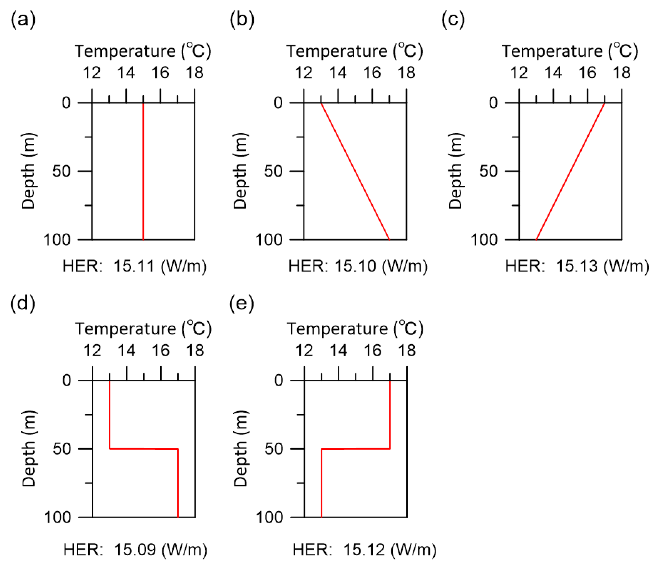
3.2.2. Subsurface Temperature

The average values of $T$ were examined. Subsurface temperature is affected not only by heat dispersion but also by the advection of groundwater flow [25,26,27,28,29,30,31]. Subsurface temperatures in the geothermal zone, which occurs at depths between 10 and 20 m, normally follow the geothermal gradient which in turn is usually represented by an increase of 1 °C per 20 to 40 m [26,32,33]. Previous studies have noted temperature anomalies at certain depths due to the artificial pumping of groundwater and temperature inversions due to global warming [33]. This study considered the five subsurface temperature profile patterns shown in Figure 8 and investigated the effect that these patterns had on the HER. The arithmetic average value of all these profiles was 15 °C. $v$ was 1e-6 m/day and ${\lambda }_s$ was 1.5 W/(mK). It was found that the HER did not change significantly in any profiles. Therefore, $T$ can be calculated as an arithmetic average.

3.2.3. Thermal Conductivity

The average of ${\lambda }_s$ was examined. The typical value of the unconsolidated sediment is from 1 to 2 W/(mK) [34]. Assuming the thermal conductivity shown in Figure 9, the effect of the change in the thermal conductivity in the depth direction on the HER was examined. The arithmetic average values of ${\lambda }_s$ were 1.5 W/(mK) in all scenarios, in which $v$ was 1.0 × 10⁻⁶ m/day and $T$ was 15 °C. In this calculation pattern, a maximum difference of 1.6% occurred comparing Figure 9a,b. The thermal conductivity of the wide area model created by Kaneko et al. [21] was 1.4 W/(mK) for the Quaternary and 1.5 W/(mK) for the Neogene. Even if arithmetic averaging is performed, it is considered to have almost no effect on the HER. Therefore, ${\lambda }_s$ can be calculated as an arithmetic average.

3.3. Creation of Estimation Formula for the HER

An estimation formula for the HER was created using the HER calculated for 33 GHE models by Kaneko et al. [21], and the three parameters $v$, $T$, and ${\lambda }_s$ input to the GHE model in Sendai Plain. These parameters are average values calculated by the method shown in Section 3.2. In this study, the regression coefficients ${\beta }_0$ to ${\beta }_9$ were determined by the least squares method to create an approximate expression using Equation (2).

Table 3. Value of regression coefficients for Equation (2) in the Sendai Plain.

${\mathit{\beta }}_0$	${\mathit{\beta }}_1$	${\mathit{\beta }}_2$	${\mathit{\beta }}_3$	${\mathit{\beta }}_4$	${\mathit{\beta }}_5$	${\mathit{\beta }}_6$	${\mathit{\beta }}_7$	${\mathit{\beta }}_8$	${\mathit{\beta }}_9$
227.12	685.41	−4.62	−270.10	−15143.42	0.02	77.18	71.44	−476.98	3.77

shows the parameters of the estimation formula, and

Table 4. Relational data between the three parameters and HER at 33 GHE models. HER calculated by the GHE model is based on Kaneko et al. [21].

No.	$\mathit{v}$	$\mathit{T}$	${\mathit{\lambda }}_{\mathit{s}}$	HER Estimate by RSM	HER Calculated by GHE Model
1	5.24 × 10−3	13.93	1.50	18.76	18.83
2	4.58 × 10−3	17.94	1.50	26.35	26.37
3	5.24 × 10−3	14.73	1.50	20.38	20.45
4	1.62 × 10−3	16.12	1.48	19.26	19.14
5	9.50 × 10−4	14.73	1.50	16.38	16.25
6	9.51 × 10−3	20.78	1.50	38.63	38.62
7	4.80 × 10−3	14.13	1.50	18.79	18.88
8	5.22 × 10−3	17.33	1.50	25.75	25.95
9	1.26 × 10−2	13.85	1.50	23.66	23.57
10	1.99 × 10−2	13.90	1.50	27.26	27.44
11	5.33 × 10−3	15.84	1.49	22.52	22.16
12	1.75 × 10−2	13.08	1.50	23.98	23.90
13	5.33 × 10−3	15.42	1.50	21.85	21.96
14	7.01 × 10−3	14.20	1.49	20.68	20.77
15	3.86 × 10−3	14.52	1.45	18.21	18.27
16	8.43 × 10−3	15.94	1.45	25.04	25.02
17	1.27 × 10−2	13.93	1.50	23.91	23.83
18	9.68 × 10−3	14.69	1.46	23.48	23.35
19	2.25 × 10−3	15.40	1.45	18.18	18.25
20	3.91 × 10−3	18.18	1.45	24.91	24.90
21	2.38 × 10−3	15.34	1.45	18.22	18.29
22	1.89 × 10−2	14.01	1.50	27.18	27.27
23	9.66 × 10−4	17.60	1.45	20.39	20.36
24	1.15 × 10−3	16.44	1.48	19.29	19.18
25	1.94 × 10−3	15.78	1.45	18.43	18.51
26	3.24 × 10−3	16.77	1.47	21.91	21.82
27	4.08 × 10−3	15.05	1.44	19.28	19.47
28	4.01 × 10−3	15.49	1.47	20.30	20.28
29	1.08 × 10−2	14.64	1.48	24.37	24.18
30	3.61 × 10−3	14.74	1.43	18.26	18.37
31	8.06 × 10−3	14.55	1.45	21.87	22.05
32	1.55 × 10−2	14.58	1.48	27.10	26.91
33	4.01 × 10−3	16.68	1.50	23.14	23.27

also shows relational data between the three parameters and HER at 33 GHE models. The HER was estimated by substituting the three parameters and regression coefficients into Equation (2). Figure 10 shows a comparison of the HER calculated by the GHE models, with one estimated by the biquadratic polynomial of the RSM (Equation (2)). The coefficient of determination between the HER calculated by the GHE models and those estimated by the RSM in the Sendai Plain was 0.999, and the root mean square error (RMSE) between these two was 0.129. It was judged that the HER estimated by the RSM was reasonable.

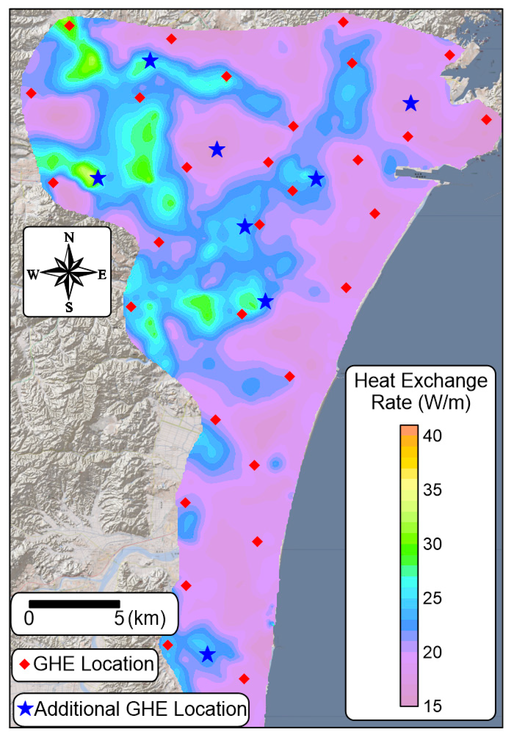
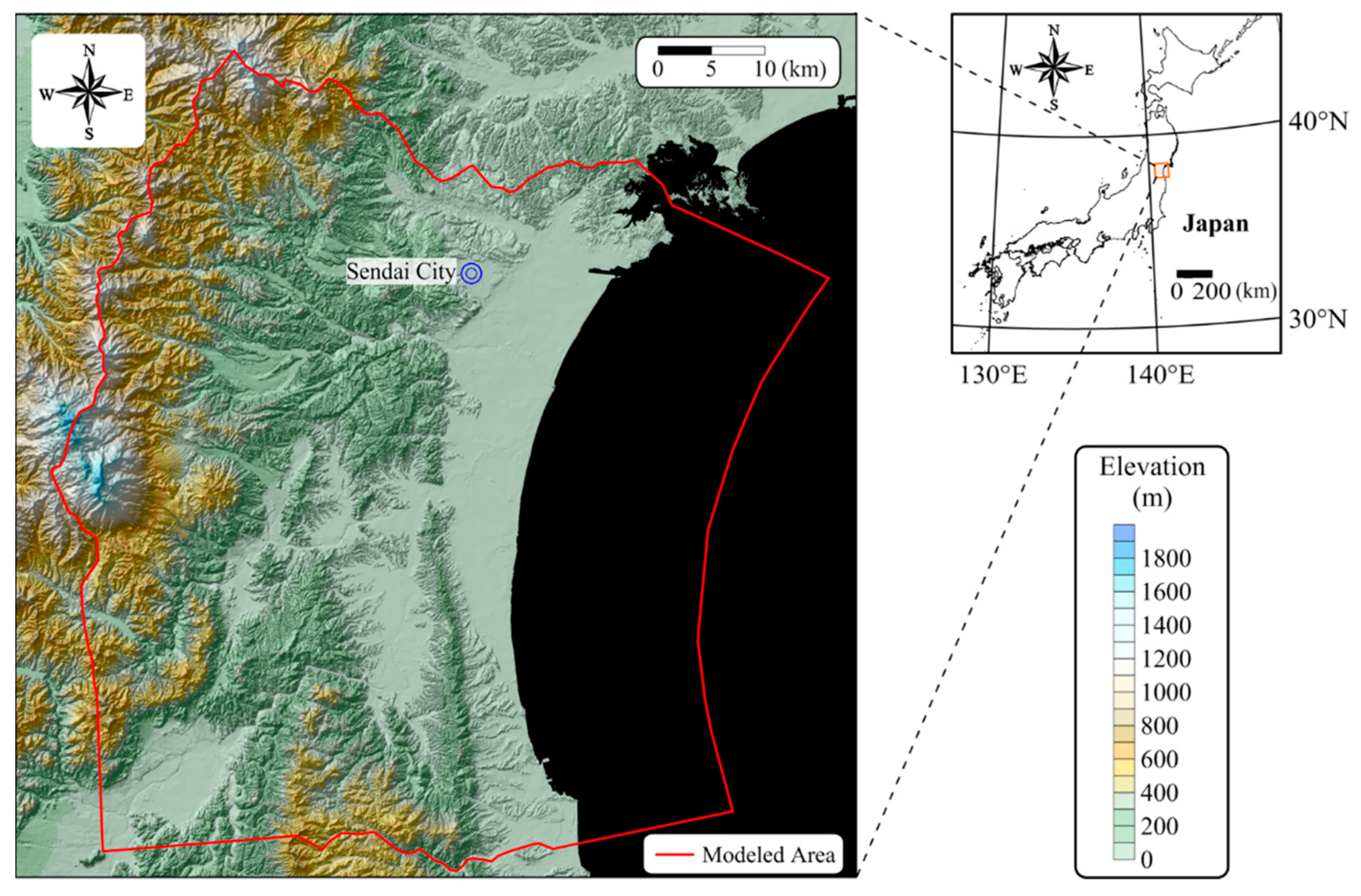
4. Application of the Estimation Formula for the HER to the Sendai Plain

The HER in the Sendai Plain was estimated based on the regional model by Kaneko et al. [21]. The average value of three parameters ($v$, $T$, and ${\lambda }_s$) from the surface to 100 m depth was extracted from meshes of the regional model, and the HER was estimated by substituting the three parameters into Equation (2). A distribution map of HER was created by performing spatial interpolation using the Kriging method on the HER estimated by each model mesh.

Figure 11 shows a comparison of the distribution map of HERs by Kaneko et al. [21] (Figure 11a, conventional map) with that estimated by the RSM (Figure 11b, refined map) in the Sendai Plain. Figure 12 also shows distribution maps of average groundwater flow velocity (Figure 12a), subsurface temperature (Figure 12b), and thermal conductivity of solids (Figure 12c) from the surface (0 m) to 100 m depth for the plain. There is little difference in the HER between the two maps at the GHE locations; however, the tendency of distribution of the HER between GHE locations was different. This is because the conventional map was created by spatial interpolation based on the HER calculated by 33 GHE locations, whereas the refined map reflects the distribution of the three parameters of $v$, $T$, and ${\lambda }_s$. It was found that the area where $v$ or $T$ was greater had a greater HER in the refined map. It was reported that the HER was strongly related to $v$ and $T$ for the plain by Kaneko et al. [21].

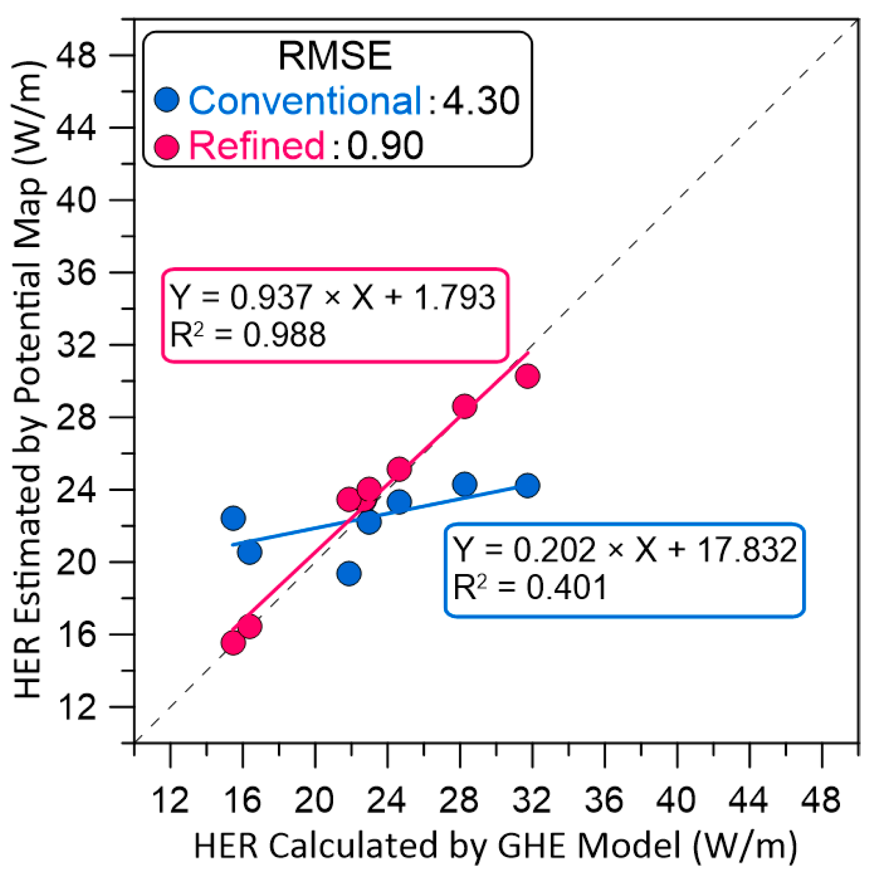
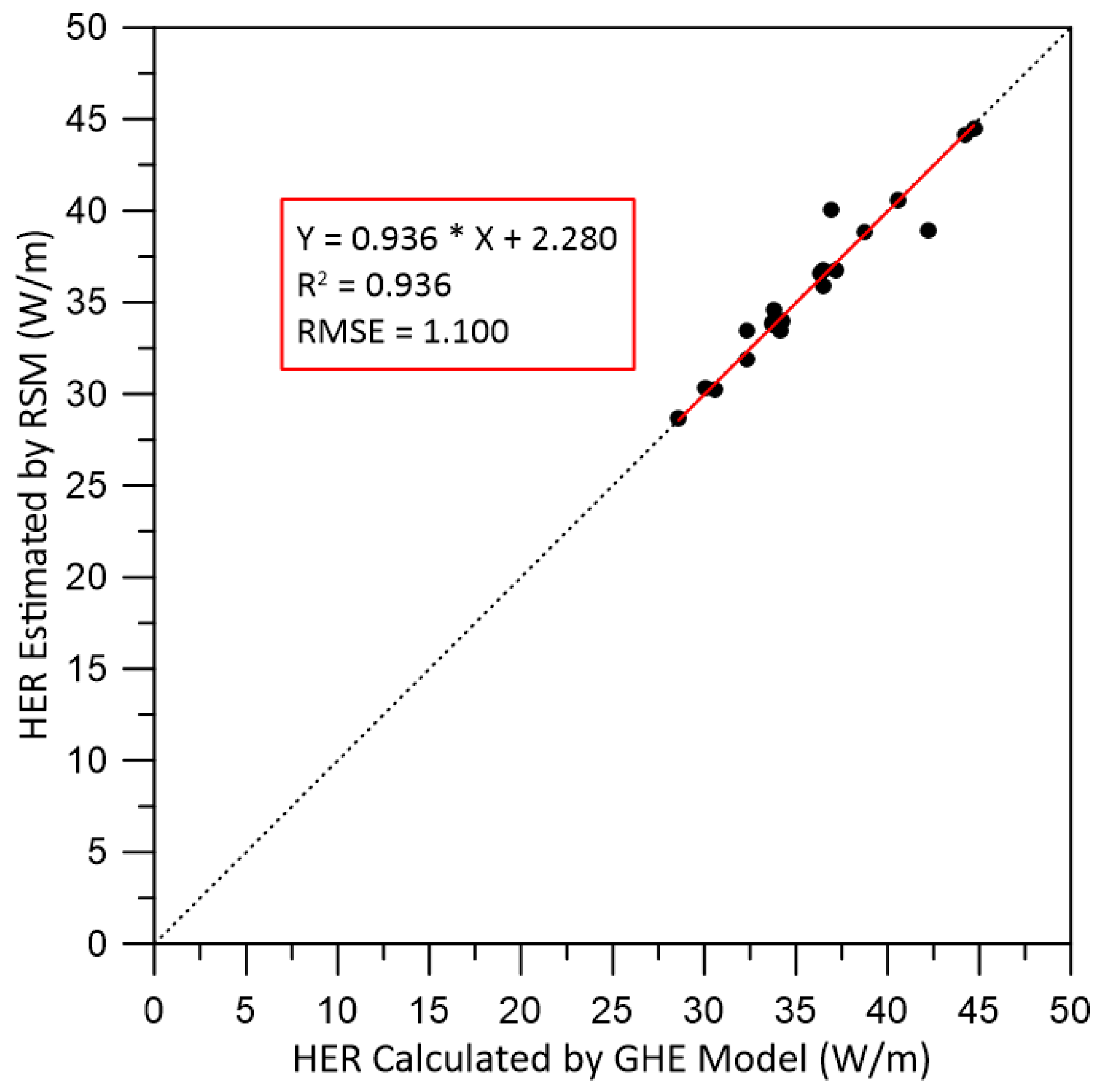
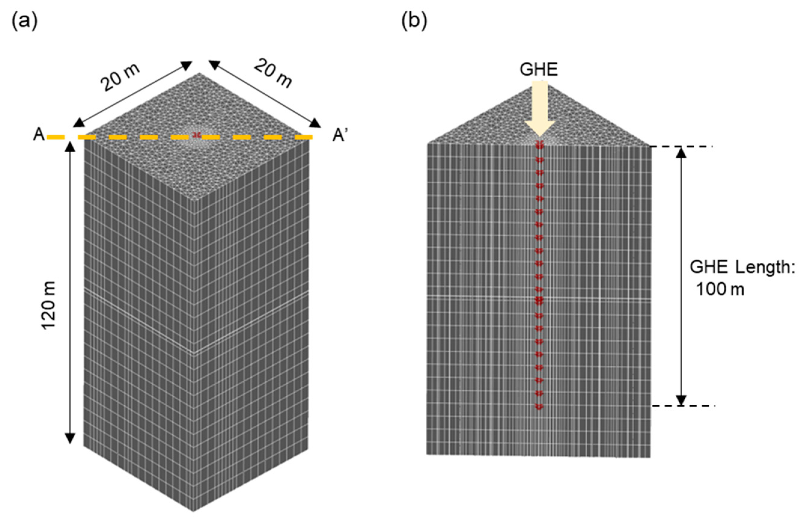
5. Validation of the Estimation Formula by Constructing GHE Models

To verify the validity of the refined map, GHE models were created at eight points (eight meshes of the regional model) where the difference in the HER between the conventional map and the improved map was relatively larger (Figure 13). The HER was calculated under the same operating conditions of the GSHP system as that used by Kaneko et al. [21]. Figure 14 shows a comparison of the HER calculated by the GHE model and the HER estimated by the RSM. The RMSE was 0.90 for the refined map and 4.30 for the conventional map. The coefficient of determination also was 0.988 for the refined map and 0.401 for the conventional map. This is because the conventional map is created by spatial interpolation based on the HER calculated at 33 GHE locations, while the refined map is created by spatial interpolation based on the HER estimated at 1273 meshes of the reginal model. Therefore, the refined map can better reflect the hydrogeological information of the regional model than the conventional map. This method cannot only create the estimation formula for the HER equivalent to the numerical analysis results but also increase the spatial resolution of the HER map.

6. Discussion

By response surface methodology, which is one kind of optimization method and a surrogate model, the HER can be estimated without heat exchange simulation by GHE model calculation (Figure 10). This proposed method can highly increase the spatial resolution of the HER map as compared to the conventional map (Figure 11). In previous studies, increasing the number of pilot points increased the time needed to create the map. However, the proposed method cannot only estimate the HER from hydrogeological parameters in an easy way but also increase the spatial resolution of the map without performing heat exchange simulations by creating a GHE model. By using this method, it is proposed that the HER can be estimated in other regions if the three parameters of $v$, $T$, and ${\lambda }_s$ can be obtained. By using the proposed method, users will have the benefit of estimating the HER with field survey data without performing numerical simulations in the future.

However, there are some challenges for applying the method to other regions. In this study, regression coefficients were calculated using the relationship between the HER and the three parameters of the GHE model in the Sendai Plain. Thus, if the three parameters outside the range of the relational data were input, misestimation of the HER may occur. Focusing on the three parameters of the 33 GHE models used to create the regression coefficient of the estimation formula for the HER, $v$ ranged from 9.5 × 10⁻⁴ to 2.0 × 10⁻² m/day, $T$ ranged from 13.1 to 20.8 °C, and ${\lambda }_s$ ranged from 1.4 to 1.5 W/(mK). When using the parameters of the regression coefficients in Table 3, the estimation formula can only be applied within the above ranges of the three hydrogeological parameters. For example, if $v$ is set to 1.0 m/day, $T$ is set to 15 °C, and ${\lambda }_s$ is set to 1.5 W/m/K, and the parameters and the regression coefficients of Table 1 are input to Equation (2), the HER is calculated as −14,085 W/m, which is an obvious mistake. As a countermeasure to this, increasing the relational data between the HER and the three variables is expected to create an estimation formula for the HER applicable to any region.

Moreover, what needs to be considered is the averaging method of the three-dimensional hydrogeological information in the depth direction, especially the averaging method of the groundwater flow velocity. In the Sendai Plain, formations in the area are mainly from the Quaternary and Neogene from the surface to a depth of 100 m, which were input to the reginal model of the Sendai Plain by Kaneko et al. [21]. In this study, the averaging method assuming the above two layers was considered. Under this condition, the HER can be estimated by using the averaging method of $v$, which is a combination of the arithmetic average and harmonic average shown in Equations (3) and (4).

Here, the proposed method was applied to 20 GHE models in the Aizu Basin, Japan constructed by Shrestha et al. [35]. The regression coefficients ${\beta }_0$ to ${\beta }_9$ were determined by the least squares method to create an approximate expression using Equation (2).

Table 5. Value of regression coefficients for Equation (2) in the Aizu Basin.

${\mathit{\beta }}_0$	${\mathit{\beta }}_1$	${\mathit{\beta }}_2$	${\mathit{\beta }}_3$	${\mathit{\beta }}_4$	${\mathit{\beta }}_5$	${\mathit{\beta }}_6$	${\mathit{\beta }}_7$	${\mathit{\beta }}_8$	${\mathit{\beta }}_9$
12.26	−2903.62	−20.39	228.72	−146.16	0.95	−48.30	187.32	444.94	−5.89

shows the parameters of the estimation formula. The HER was estimated by substituting three parameters and regression coefficients into Equation (2). Figure 15 shows a comparison of the HER calculated by the GHE models with that estimated by the biquadratic polynomial of the RSM (Equation (2)). The coefficient of determination between the HER calculated by the GHE models and those estimated by the RSM in the Sendai Plain was 0.936, and the RMSE between the two in the Sendai Plain was 1.100. The estimation accuracy of the HER in the basin was not better than that in the plain. This is because the input parameters to the GHE models in the vertical direction between the two regions were different. In the plain, the input parameters were changed by the boundary between Quaternary and Neogene. In contrast, they were changed by 10 m depth in the basin.

Figure 16 shows the temperature distribution in the GHE of the uniform model, two-layer model, and 10-layer model and the HER when the arithmetic average groundwater flow velocity was 0.22 m/day. The HER was 63.27 W/m when the $v$ was 0.22 m/day (Figure 16a) constantly. When the velocity from the surface to 50 m depth ($v_1$) was 0.4 m/day and the velocity from a depth of 50 m to 100 m ($v_2$) was 0.04 m/day, the HER was 57.68 W/m (Figure 16b). However, when $v_1$ was 0.4 m/day and $v_2$ was 0.04 m/day, which were entered alternately every 10 m in depth, the HER was 61.34 W/m (Figure 16c). The averages in the conditions of Figure 16b,c are both calculated as arithmetic average of 0.22 m/day and the harmonic average of 7.3 × 10⁻² m/day. The same HER was estimated using the optimization method under the conditions in Figure 16b,c. This is because Equations (3) and (4) for averaging $v$ are calculated by a combination of arithmetic average and harmonic average; therefore, they have the same average groundwater flow velocity, that is, the same HER is obtained under the conditions in Figure 16b,c. Equations (3) and (4) are intended for the two-layer model (Sendai Plain hydrogeological model), so it is necessary to create another averaging equation not only for the 10-layer model but also for other models, which is a content of further study.

From the above, using the proposed optimization method cannot only estimate the HER from hydrogeological parameters in an easy way but also highly increase the spatial resolution of a map by creating a GHE model without performing heat exchange simulation. The creation of the potential maps in various regions can be expected by using this method and by increasing the relational data between the HER and hydrogeological parameters. To create a universal estimation formula for the HER, it is necessary to consider the averaging method that matches the hydrogeological model of each region, which is a content of further study.

7. Conclusions

This study proposed an estimation formula for the HER to obtain a solution equivalent to the numerical analysis result considering the average method when supplying 3D hydrogeological information affecting HER to a 2D map. The results of the study are enumerated below:

(1)

It was found that the main factors affecting the HER were groundwater flow velocity ($v$), subsurface temperature ($T$), and thermal conductivity of solids (${\lambda }_s$).

(2)

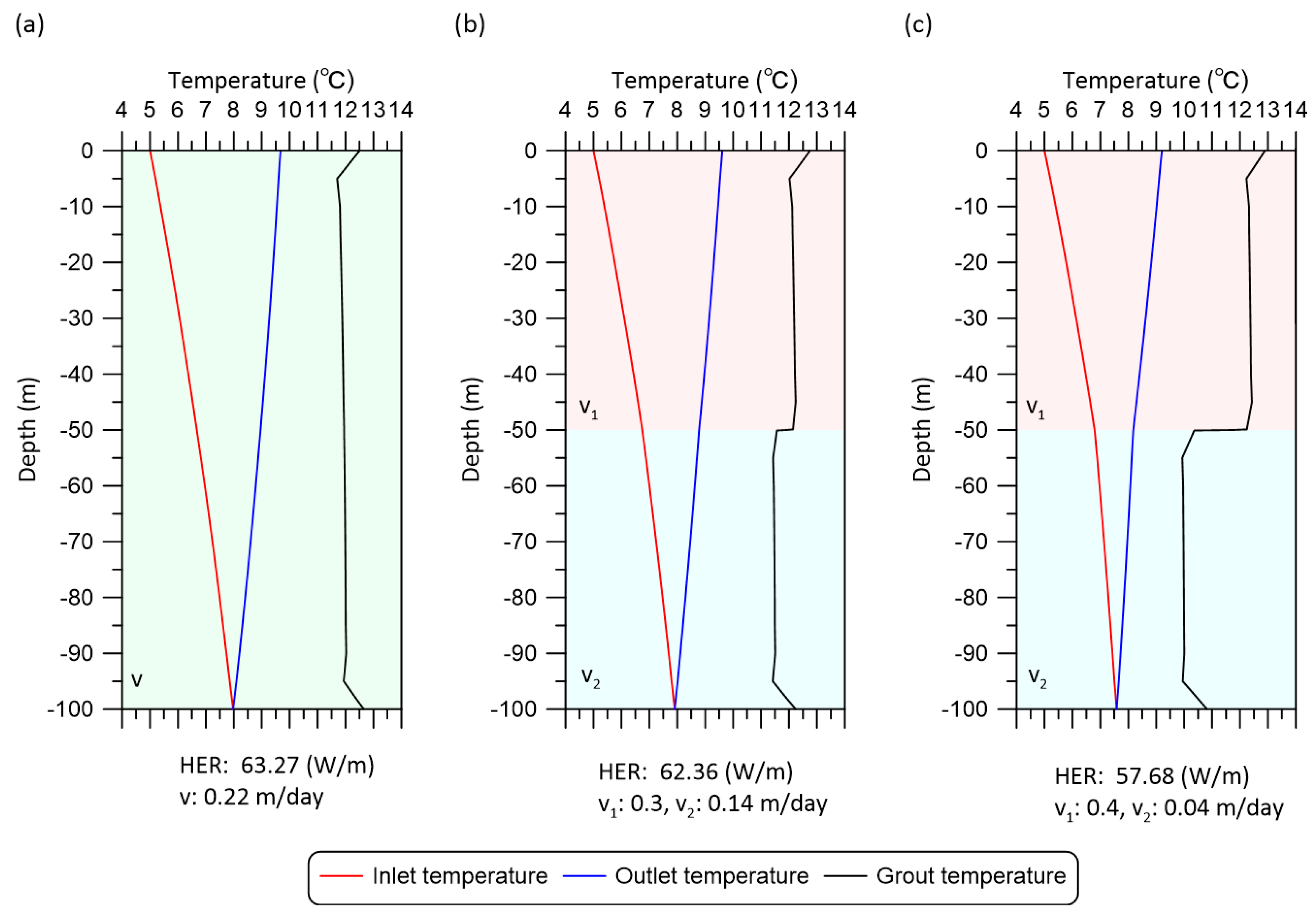
The average method in the vertical direction (GHE length) was evaluated. $T$ and ${\lambda }_s$ can be calculated by arithmetic averaging. In contrast, $v$ has to be calculated as a combination of arithmetic and harmonic average.

(3)

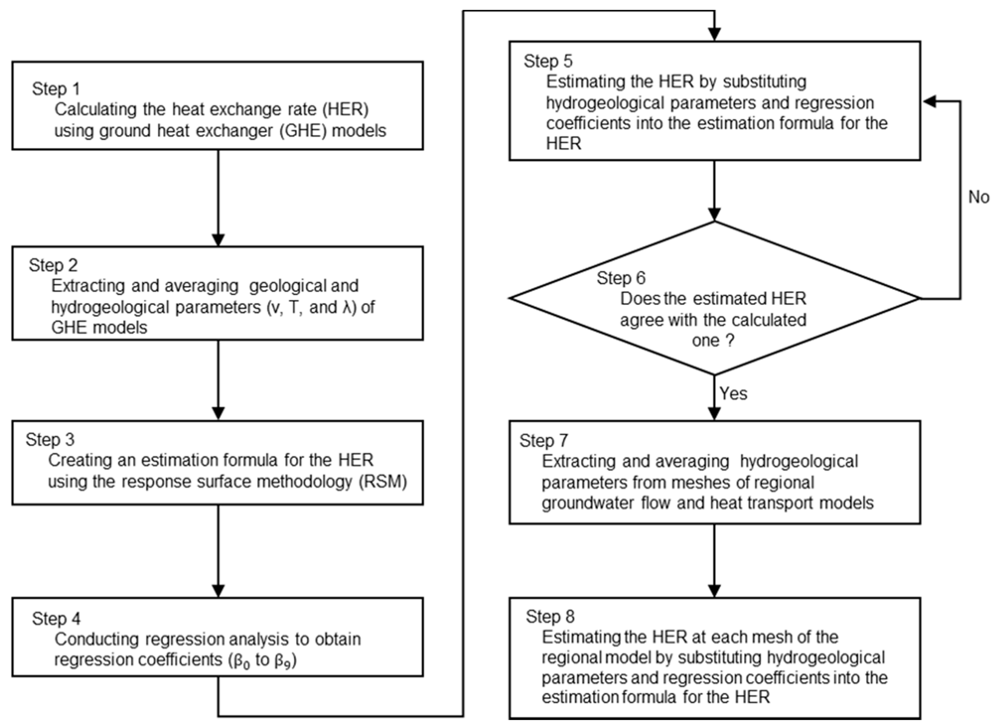
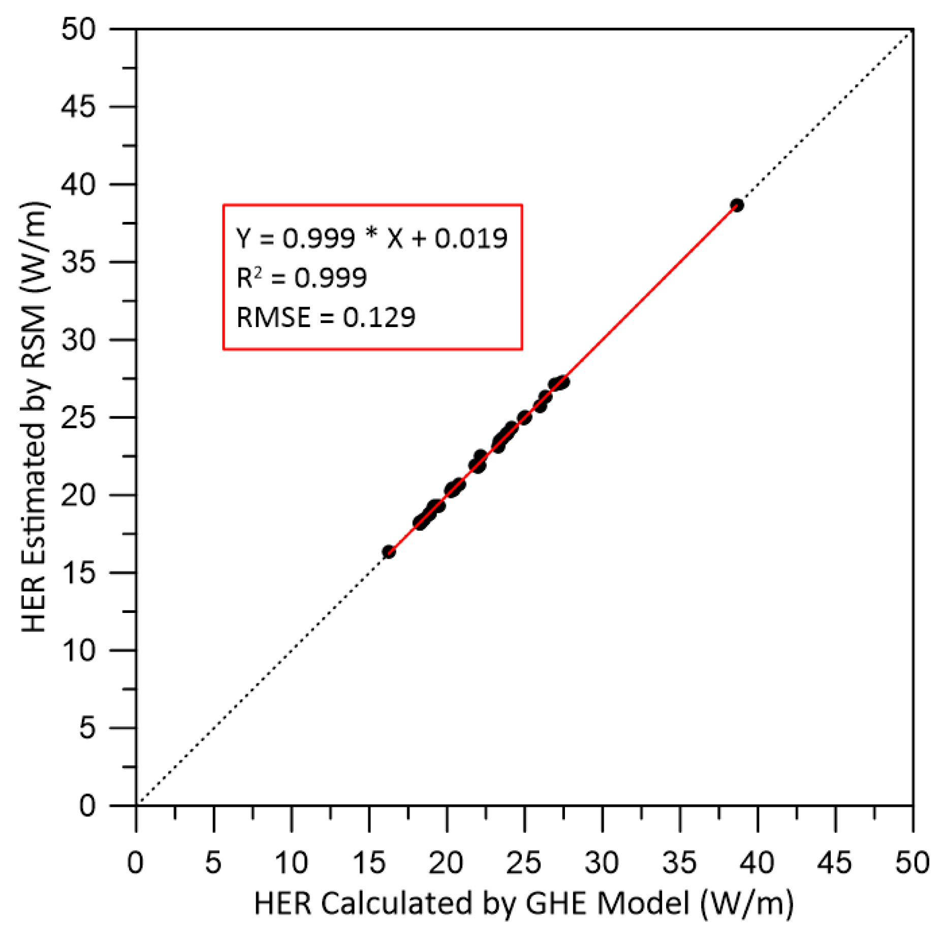
The RSM was utilized to approximate the HER using the three parameters in the Sendai Plain. The estimated HER agreed well with the calculated one by the GHE models because the coefficient of determination and RMSE between the two HERs were 0.999 and 0.129, respectively.

(4)

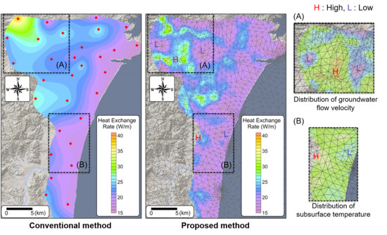
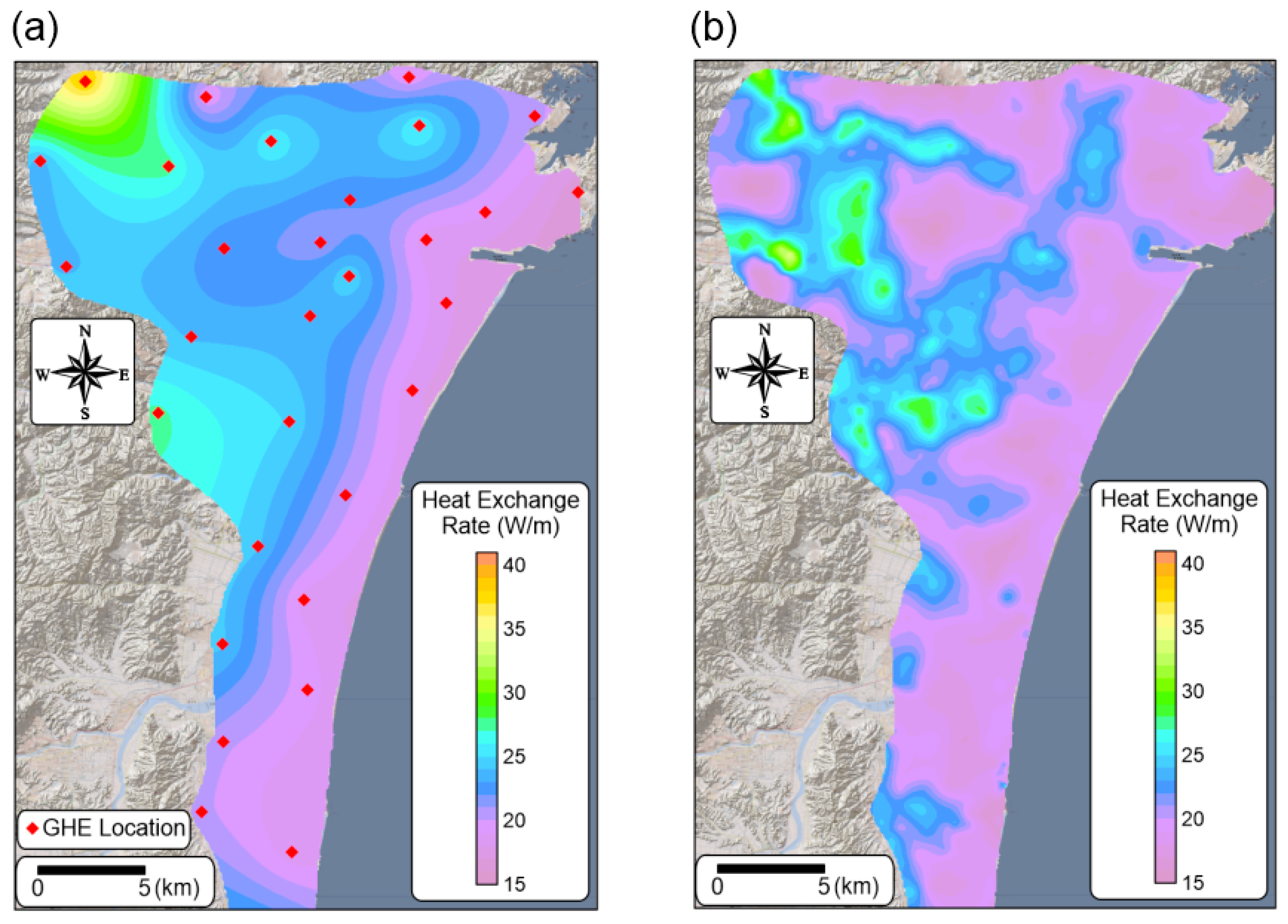
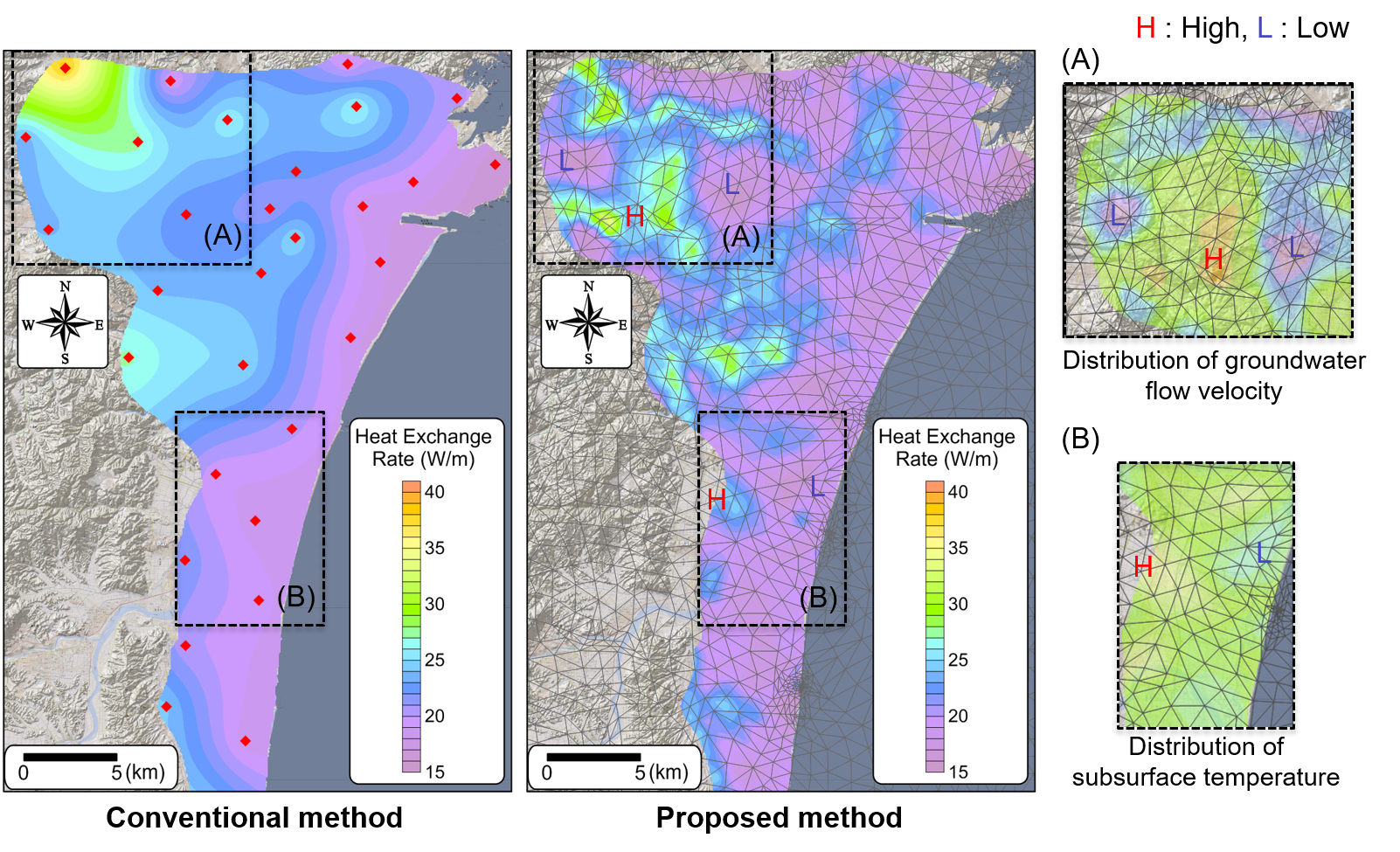
The proposed method cannot only estimate the HER from hydrogeological parameters in an easy way but also highly increase the spatial resolution of a map by creating a GHE model without performing heat exchange simulations.

It should be noted that the proposed method of suitable evaluation combining numerical simulation and mathematical optimization methods is unique to this study. This method can achieve higher accuracies in a shorter time compared to previous methods, which can help selecting suitable locations for GSHP system installations more effectively and promoting such systems in Japan.

For future study, an averaging method that matches the hydrogeological model of each region will be examined to create a universal estimation formula for the HER, leading to a potential map of GSHP systems throughout Japan that will increase the number of GSHP system installations.

References

1. Fujii, H.; Inatomi, T.; Itoi, R.; Uchida, Y. Development of suitability maps for ground-coupled heat pump systems using groundwater and heat transport models. Geothermics 2007, 36, 459–472. [Google Scholar] [CrossRef]
2. Mustafa Omer, A. Ground-source heat pumps systems and applications. Renew. Sustain. Energy Rev. 2008, 12, 344–371. [Google Scholar] [CrossRef]
3. Wagner, V.; Bayer, P.; Kübert, M.; Blum, P. Numerical sensitivity study of thermal response tests. Renew. Energy 2012, 41, 245–253. [Google Scholar] [CrossRef]
4. Self, S.J.; Reddy, B.V.; Rosen, M.A. Geothermal heat pump systems: Status review and comparison with other heating options. Appl. Energy 2013, 101, 341–348. [Google Scholar] [CrossRef]
5. Ozgener, O.; Hepbasli, A. Modeling and performance evaluation of ground source (geothermal) heat pump systems. Energy Build. 2007, 39, 66–75. [Google Scholar] [CrossRef]
6. Salvalai, G. Implementation and validation of simplified heat pump model in IDA-ICE energy simulation environment. Energy Build. 2012, 49, 132–141. [Google Scholar] [CrossRef]
7. Perego, R.; Guandalini, R.; Fumagalli, L.; Aghib, F.S.; De Biase, L.; Bonomi, T. Sustainability evaluation of a medium scale GSHP system in a layered alluvial setting using 3D modeling suite. Geothermics 2016, 59, 14–26. [Google Scholar] [CrossRef]
8. Dalla Santa, G.; Galgaro, A.; Sassi, R.; Cultrera, M.; Scotton, P.; Mueller, J.; Bertermann, D.; Mendrinos, D.; Pasquali, R.; Perego, R.; et al. An updated ground thermal properties database for GSHP applications. Geothermics 2020, 85, 101758. [Google Scholar] [CrossRef]
9. Han, C.; Yu, X. Sensitivity analysis of a vertical geothermal heat pump system. Appl. Energy 2016, 170, 148–160. [Google Scholar] [CrossRef] [Green Version]
10. Li, C.; Cleall, P.J.; Mao, J.; Muñoz-Criollo, J.J. Numerical simulation of ground source heat pump systems considering unsaturated soil properties and groundwater flow. Appl. Therm. Eng. 2018, 139, 307–316. [Google Scholar] [CrossRef]
11. Cheap-Gshps Cheap and Efficient Application of Reliable Ground Source Heat Exchangers and Pumps. Available online: https://cheap-gshp.eu/ (accessed on 25 February 2020).
12. Luo, J.; Luo, Z.; Xie, J.; Xia, D.; Huang, W.; Shao, H. Investigation of shallow geothermal potentials for different types of ground source heat pump systems (GSHP) of Wuhan city in China. Renew. Energy 2018, 118, 230–244. [Google Scholar] [CrossRef]
13. Shrestha, G.; Uchida, Y.; Yoshioka, M.; Fujii, H.; Ioka, S. Assessment of development potential of ground-coupled heat pump system in Tsugaru Plain, Japan. Renew. Energy 2015, 76, 249–257. [Google Scholar] [CrossRef]
14. Shrestha, G.; Uchida, Y.; Kuronuma, S.; Yamaya, M.; Katsuragi, M.; Kaneko, S.; Shibasaki, N.; Yoshioka, M. Performance evaluation of a ground-source heat pump system utilizing a flowing well and estimation of suitable areas for its installation in Aizu Basin, Japan. Hydrogeol. J. 2017, 25, 1437–1450. [Google Scholar] [CrossRef]
15. Fujii, H.; Itoi, R.; Fujii, J.; Uchida, Y. Optimizing the design of large-scale ground-coupled heat pump systems using groundwater and heat transport modeling. Geothermics 2005, 34, 347–364. [Google Scholar] [CrossRef]
16. Zanchini, E.; Lazzari, S.; Priarone, A. Long-term performance of large borehole heat exchanger fields with unbalanced seasonal loads and groundwater flow. Energy 2012, 38, 66–77. [Google Scholar] [CrossRef]
17. Choi, J.C.; Park, J.; Lee, S.R. Numerical evaluation of the effects of groundwater flow on borehole heat exchanger arrays. Renew. Energy 2013, 52, 230–240. [Google Scholar] [CrossRef]
18. Dehkordi, S.E.; Schincariol, R.A. Effect of thermal-hydrogeological and borehole heat exchanger properties on performance and impact of vertical closed-loop geothermal heat pump systems. Hydrogeol. J. 2014, 22, 189–203. [Google Scholar] [CrossRef]
19. Casasso, A.; Sethi, R. Efficiency of closed loop geothermal heat pumps: A sensitivity analysis. Renew. Energy 2014, 62, 737–746. [Google Scholar] [CrossRef] [Green Version]
20. Environmental Management Bureau, Government of Japan. Ministry of the Environment Results of a Survey on the Installation Conditions of Ground-Source Heat Pump Systems. Available online: http://www.env.go.jp/press/106636.html (accessed on 25 February 2020). (In Japanese)
21. Kaneko, S.; Uchida, Y.; Shrestha, G.; Ishihara, T.; Yoshioka, M. Factors affecting the installation potential of ground source heat pump systems: A comparative study for the Sendai plain and Aizu basin, Japan. Energies 2018, 11, 2860. [Google Scholar] [CrossRef] [Green Version]
22. Diersch, H.-J.G. FEFLOW—Finite Element Modeling of Flow, Mass and Heat Transport in Porous and Fractured Media; Springer: Berlin/Heidelberg, Germany, 2014; ISBN 978-3-642-38738-8. [Google Scholar]
23. Tomigashi, A.; Nishiyama, K.; Yamamoto, A.; Dan, T.; Takahashi, T. Proposal of method evaluating installation potential of ground source heat pump systems in regional area. In Proceedings of the 2013 spring meeting Japanese Association of Groundwater Hydrology Abstracts with Programs, Chiba, Japan, 18 May 2013; pp. 104–109. (In Japanese). [Google Scholar]
24. Vu-Bac, N.; Lahmer, T.; Zhuang, X.; Nguyen-Thoi, T.; Rabczuk, T. A software framework for probabilistic sensitivity analysis for computationally expensive models. Adv. Eng. Softw. 2016, 100, 19–31. [Google Scholar] [CrossRef]
25. Smith, L.; Chapman, D.S. On the thermal effects of groundwater flow, 1. Regional scale systems. J. Geophys. Res. 1983, 88, 593–608. [Google Scholar] [CrossRef]
26. Anderson, M.P. Heat as a ground water tracer. Ground Water 2005, 43, 951–968. [Google Scholar] [CrossRef] [PubMed]
27. Saar, M.O. Review: Geothermal heat as a tracer of large-scale groundwater flow and as a means to determine permeability fields. Hydrogeol. J. 2011, 19, 31–52. [Google Scholar] [CrossRef]
28. Alcaraz, M.; García-Gil, A.; Vázquez-Suñé, E.; Velasco, V. Advection and dispersion heat transport mechanisms in the quantification of shallow geothermal resources and associated environmental impacts. Sci. Total Environ. 2016, 543, 536–546. [Google Scholar] [CrossRef]
29. Majumder, R.K.; Shimada, J.; Taniguchi, M. Groundwater flow systems in the Bengal Delta, Bangladesh, inferred from subsurface temperature readings. Songklanakarin J. Sci. Technol. 2013, 35, 99–106. [Google Scholar]
30. Domenico, P.A.; Palciauskas, V.V. Theoretical analysis of forced convective heat transfer in regional ground-water flow. Bull. Geol. Soc. Am. 1973, 84, 3803–3814. [Google Scholar] [CrossRef]
31. Taniguchi, M.; Williamson, D.R.; Peck, A.J. Disturbances of temperature-depth profiles due to surface climate change and subsurface water flow: 2. An effect of step increase in surface temperature caused by forest clearing in southwest Western Australia. Water Resour. Res. 1999, 35, 1519–1529. [Google Scholar] [CrossRef]
32. Parsons, M.L. Groundwater thermal regime in a glacial complex. Water Resour. Res. 1970, 6, 1701–1720. [Google Scholar] [CrossRef]
33. Yasukawa, K.; Uchida, Y.; Tenma, N.; Taguchi, Y.; Muraoka, H.; Ishii, T.; Suwanlert, J.; Buapeng, S.; Nguyen, T.H. Groundwater temperature survey for geothermal heat pump application in tropical Asia. Bull. Geol. Surv. Japan 2009, 60, 459–467. [Google Scholar] [CrossRef]
34. Domenico, P.A.; Schwartz, F.W. Physical and Chemical Hydrogeology; John Wiley & Sons, Inc.: Hoboken, NJ, USA, 1990. [Google Scholar]
35. Shrestha, G.; Uchida, Y.; Ishihara, T.; Kaneko, S.; Kuronuma, S. Assessment of the installation potential of a ground source heat pump system based on the groundwater condition in the Aizu Basin, Japan. Energies 2018, 11, 1178. [Google Scholar] [CrossRef] [Green Version]
Figure 1. Study area and modeled area quoted from Kaneko et al. [21]. The relief map and elevation data are drawn using the 10 m grid digital elevation map sourced from the Geospatial Information Authority of Japan (GSI).
Energies 13 01872 g001
Figure 2. Three-dimensional (3D) groundwater flow and heat transport model of the Sendai Plain (reginal model) quoted from Kaneko et al. [21].
Energies 13 01872 g002
Figure 3. Ground heat exchanger (GHE) model. (a) Bird’s-eye view (b) cross-sectional view at A–A’.
Energies 13 01872 g003
Figure 4. Flowchart of the proposed method in this paper.
Energies 13 01872 g004
Figure 5. Temperature distribution in the borehole and result of GHE simulation. Groundwater flow velocity was set as (a) v : 0.22 m/day, (b) v 1 : 0.3 m/day and v 2 : 0.14 m/day, and (c) v 1 : 0.4 m/day and v 2 : 0.04 m/day.
Energies 13 01872 g005
Figure 6. Relationship between groundwater flow velocity and heat exchange rate in the uniform model.
Energies 13 01872 g006
Figure 7. Relationship between arithmetic average groundwater flow velocity and (a) parameters α and (b) β.
Energies 13 01872 g007
Figure 8. Distribution of the subsurface temperature profile and GHE simulation result of the model. The temperature profile was set as (a) 15 °C, (b) with a temperature gradient of 0.04 °C/m, (c) temperature gradient of −0.04 °C/m, (d) 13 °C from top to 50 m depth and 17 °C from 50 to 100 m depth, and (e) 17 °C from top to 50 m depth and 13 °C from 50 to 100 m depth. The arithmetic average value of all these profiles was 15 °C.
Energies 13 01872 g008
Figure 9. Distribution of thermal conductivity and simulation result of the GHE model. The distribution was set as (a) 1.5 W/(mK), (b) 1.0 W/(mK) from top to 50 m depth and 2.0 W/(mK) from 50 to 100 m depth, (c) 1.3 W/(mK) from top to 50 m depth and 1.7 W/(mK) from 50 to 100 m depth, (d) 1.7 W/(mK) from top to 50 m depth and 1.3 W/(mK) from 50 to 100 m depth, and (e) 2.0 W/(mK) from top to 50 m depth and 1.0 W/(mK) from 50 to 100 m depth. The arithmetic average values of thermal conductivity were 1.5 W/(mK) in all scenarios.
Energies 13 01872 g009
Figure 10. Comparison of the heat exchange rate calculated by the GHE models with that estimated by the RSM in the Sendai Plain. HER, GHE, and RSM denote the heat exchange rate, ground heat exchanger, and response surface methodology, respectively.
Energies 13 01872 g010
Figure 11. Comparison of (a) distribution map of heat exchange rates by Kaneko et al. [21]; conventional map with (b) that estimated by the RSM; refined map for the Sendai Plain.
Energies 13 01872 g011
Figure 12. Distribution maps of (a) average groundwater flow velocity, (b) average subsurface temperature, and (c) average thermal conductivity of solids from the surface (0 m) to 100 m depth for the Sendai Plain.
Energies 13 01872 g012
Figure 13. Additional GHE location in the Sendai Plain.
Energies 13 01872 g013
Figure 14. Comparison of the heat exchange rate calculated by GHE models with that estimated by the RSM in the Sendai Plain.
Energies 13 01872 g014
Figure 15. Comparison of the heat exchange rate calculated by GHE models with that estimated by the RSM in the Aizu Basin. HER, GHE, and RSM denote heat exchange rate, ground heat exchanger and response surface methodology, respectively.
Energies 13 01872 g015
Figure 16. Temperature distribution in the borehole and result of the GHE simulation. Groundwater flow velocity was set as (a) v : 0.22 m/day, (b) v 1 : 0.4 m/day at depth of 0 to 50 m and v 2 : 0.04 m/day at depth of 50 to 100 m, and (c) v 1 : 0.4 m/day and v 2 : 0.04 m/day, which are entered alternately every 10 m in depth. Figure 16a is the same as Figure 5a, and Figure 16b is the same as Figure 5c.
Energies 13 01872 g016