Active Disturbance Rejection Control of a Longitudinal Tunnel Ventilation System

Abstract

This paper proposes an innovative approach for controlling pollutant release in a long-distance tunnel via longitudinal ventilation. Enhanced by an active disturbance rejection control (ADRC) method, a ventilation controller is developed to regulate the forced air ventilation in a road tunnel. As a result, the pollutants (particulate matter and carbon monoxide) are reduced by actively regulating the air flow rate through the tunnel. The key contribution of this study lies in the development of an extended state observer that can track the system disturbance and provide the system with compensation via a nonlinear state feedback controller equipped by the ADRC. The proposed method enhances the disturbance attenuation capability in the ventilation system and keeps the pollutant concentration within the legitimate limit in the tunnel. In addition to providing a safe and clean environment for passengers, the improved tunnel ventilation can also achieve better energy saving as the air flow rate is optimized.

1. Introduction

Longitudinal ventilation systems are widely used in long-distance tunnels for air ventilation. Generally, moving vehicles in tunnels bring about air circulation from the entrance to exit. However, when the traffic is heavy and the meteorological pressure differences are low, there is a need to operate tunnel ventilators to keep pollutant concentrations below the relevant limit. Thus, there is a balance to strike between the minimal use of electricity for fan ventilators and high air quality in the tunnel because of the existence random and chaotic factors. The pollutants in the air are randomly ejected in the tunnel by incoming vehicles whilst the wind load varies in time and direction. Uncertainty and nonlinear factors make it difficult to accurately model the aerodynamics of the air and the diffusion of the pollutants within the tunnel. Therefore, a model-based control scheme cannot perform effectively in these cases.

In the literature, fuzzy logic [1] is introduced to deal with the nonlinearity and complexity of the ventilation system, and applied in the actual tunnel. The results show that energy saving is achieved whilst improving the tunnel air quality. Fuzzy control has become a popular option in ventilation control schemes. In order to improve the performance of fuzzy logic control, many scholars have developed a number of technologies. Koyama et al. [2] used the minimum power consumption of the ventilation equipment as the optimization target and solved the problems using nonlinear programming with fuzzy control. As a result, an optimal scheme to determine the number of running ventilators was developed [2]. Chu et al. developed a fuzzy controller enhanced by a genetic algorithm to maintain the concentration of pollutants at a certain level and to minimize power consumption [3]. Bogdan et al. combined model prediction with fuzzy control [4]. By measuring traffic intensity, weather conditions and tunnel parameters, the predictive controller estimated fresh air requirements and calculated the number of required fans, while the fuzzy controller compared measured and admissible levels of pollutants and adjusted a predicted number of jet fans to keep pollutant levels within predefined thresholds. Alternatively, Euler-Rolle and Fuhrmann et al. designed a specially structured non-linear observer in a feedback and feed-forward ventilation control system to estimate and compensate for external disturbances that tunnels are subjected to [5,6]. Euler-Rolle and Fuhrmann et al. considered the dynamic behavior of the air flow velocity for an emergency with fire and smoke, and then designed the feed-forward and feedback controller, adding an additional observer. This observer and the controller were designed separately. The observed disturbances were incorporated into the feed-forward control signals to enhance the disturbance attenuation ability of the control scheme for large and sudden pressure drops. Through the compensation of this non-linear observer, the control scheme performed better than the control schemes based on the fuzzy logic. In reference [7], an adaptive control scheme incorporating fuzzy logic proved to be effective in handling nonlinearity problems.

Traditionally, proportion integration differentiation (PID) control is widely used in system operation [8,9] owing to its simplicity and robustness to the disturbance. However, when the systems suffer from complex uncertainty and nonlinearity, PID struggles to achieve optimal solutions. Fuzzy logic and model-free methods are useful to deal with nonlinearity. However, they usually rely on the empirical and historical information from previous operation. Their performance may deteriorate when new disturbances occur. In this case, active disturbance rejection control is a good option to cope with these issues.

Based on the concept of active disturbance rejection control (ADRC) [10], a new control strategy for ventilation operation is proposed to cope with the model uncertainties and disturbances. ADRC realizes the organic fusion of the observer and the nonlinear controller. Applications of ADRC can be found in a variety of fields, including power [11,12,13], motion [14,15,16], and process control [17,18]. In normal ventilation operation, the control of pollutant concentration is the ultimate goal, and the control of the air flow velocity is used to exhaust the pollutants. In these cases, a ventilation control system is described by two serial-connected subsystems to control the diffusion of pollutant concentration and the in-tunnel air flow. The novelty of this study lies in that an ADRC is used to design the two cascade controllers. In this way, the reference of the control variables in the first subsystem can be derived from the output of the second subsystem. The advantage of this back-stepping technique is gained in this study where the air flow velocity is taken into account as a pseudo control variable. Once determined, it is used as the set point by the second ADRC controller. Parameter uncertainties or model errors in line with these two subsystem models are corrected by a nonlinear controller equipped with ADRC. By tracking the reference, an extended state observer (ESO) compensates for the inaccuracies and improves the control performance. The configuration of the ventilation control system is depicted in Figure 1. It consists of a plant (a tunnel system), an air flow velocity controller, two pollutant concentration observers, and a number of measurement devices.

This paper is structured as follows: Section 2 presents the non-linear dynamical model of a tunnel ventilation system with some assumptions. Section 3 gives a brief introduction of an ADRC scheme. The design procedure of the cascade subsystems in relation to the tunnel ventilation system is given in Section 4. Section 5 presents simulation results by comparison with the existing method used in the Zhongliangshan tunnel, China. Finally, the key findings and contributions are summarized in Section 6.

2. Dynamical Model of a General Tunnel System with Nonlinear Method

A general tunnel system is very complex and no simple model can be designed for it. To handle the system more easily, Kurka et al. and Ferkl and Meinsma, performed a functional decomposition [19,20]; therefore, the tunnel model comprises three main functional parts (or subsystems)—ventilation, traffic and exhaust.

2.1. Ventilation model based on generalized Bernoulli equation

Consider a one-dimensional model with lumped parameters, meaning the airflow velocity $v_a$ does not depend on the $y$ and $z$ coordinates, i.e., $\frac{\partial v_a}{\partial y}=\frac{\partial v_a}{\partial z}=0$. For simplification purposes, consider the incompressible flow, meaning the density of air $\mathsf{\rho }$ is constant along the entire length of the tunnel and does not depend on time.

A road tunnel can be divided into sections with constant geometry, cross-section area, hydraulic diameter, etc. Based on the assumptions stated above, the airflow velocity is constant within the whole section. The airflow dynamics in each section is described by the generalized Bernoulli equation.

The generalized Bernoulli equation for incompressible and unsteady flow can be expressed in different ways. For this purpose, the following equation is used [21,22]:

$$\rho ·L·\frac{d{v}_a}{dt}=\Delta P$$

(1)

where $\frac{d{v}_a}{dt}$ represents the acceleration of airflow, $L$ is the length of the given section of the tunnel, $\rho$ is the density of air, $v_a$ is the airflow velocity, and $\Delta P$ denotes the total pressure change in the given section of the tunnel.

The total pressure change $\Delta P$ in the given section of the tunnel can be divided into pressure losses caused by air friction $\Delta P_{fric}$, changes in tunnel geometry $\Delta P_{area}$, pressure change due to running jet fans $\Delta P_{JF}$, piston effect force of vehicles $\Delta P_{pist}$, and disturbance effects $\Delta P_{wind}$ caused by natural wind:

$$\Delta P=\Delta P_{JF}+\Delta P_{pist}-\Delta P_{fric}-\Delta P_{area}-\Delta P_{wind}$$

(2)

The pressure drop $\Delta P_{area}$ caused by local losses depends on a loss coefficient $\zeta$, which represents losses due to the cross section changes, the shape of transition, the direction of flow, etc., as in Equation (3):

$$\Delta P_{area}=\frac{\rho }{2}·\left({\zeta }_{in}+{\zeta }_{out}\right)·v_a^2$$

(3)

where $\Delta P_{area}$ mainly undergoes two types of losses caused by cross section changes. One kind is the contraction loss at the entrance $\Delta P_{in}=\frac{\rho }{2}·{\zeta }_{in}·v_a^2$; the other is expansion loss at the outlet $\Delta P_{out}=\frac{\rho }{2}·{\zeta }_{out}·v_a^2·{\zeta }_{in}$ denotes the contraction head loss coefficient at the tunnel entrance, and ${\zeta }_{out}$ describes the expansion head loss coefficient at the outlet of the tunnel.

The pressure drop $\Delta P_{fric}$ caused by friction losses depends on wall roughness, traffic signs on the walls, etc. $\Delta P_{fric}$ can be calculated as:

$$\Delta P_{fric}=\frac{\rho }{2}·\lambda ·\frac{L}{D_H}·v_a^2$$

(4)

where $\lambda$ represents the coefficient friction of the tunnel walls, and $D_H$ is the hydraulic diameter of the tunnel.

The pressure drop $\Delta P_{pist}$ caused by the piston effect of the vehicles represents the influence of the vehicles passing through the tunnel, shown by Equation (5):

$$\Delta P_{pist}=\frac{\rho }{2}·\frac{L}{A_{Tun}·v_{veh}}·\left(v_{veh}-v_a\right)·\left|v_{veh}-v_a\right|·{\gamma }_{conv}·{\displaystyle \sum }_{i=1}^m{S}_i·n_i$$

(5)

where $v_{veh}$ represents the average speed of the vehicles, $A_{Tun}$ describes the tunnel cross section area, $S_i$ is the average head surface area of the $i_{th}$ vehicle type, $n_i$ is the number of vehicles of the $i_{th}$ type, and ${\gamma }_{conv}$ defines the convoy polynomial [23].

The pressure drop $\Delta P_{JF}$ describes the effect of the $N_{JV}$ jet fans on the flow velocity, shown by Equation (6):

$$\Delta P_{JF}=\Delta P_{JF\_i}·N_{JV}$$

(6)

$$\Delta P_{JF\_i}=k_{JV\_i}·v_{JV\_i}^2·\left(1-\frac{v_a}{v_{JV\_i}}\right)$$

(7)

The pressure drop $\Delta P_{JF\_i}$ indexed by $i$ is characterized by the average outlet velocity $v_{JV\_i}$ and the factor $k_{JV\_i}$ of each jet fan:

$$k_{JV\_i}=\rho ·\frac{A_{JV\_i}}{A_{Tun}}·k_{e\_i}$$

(8)

where $A_{JV\_i}$ is the cross sectional area of the $i_{th}$ ventilator, and $k_{e\_i}$ is the correction factor taking account of the installation situation for the $i_{th}$ ventilator [5].

Additionally, the wind acting on the tunnel port affects the air flow in the tunnel dependent on the wind speed $v_{wind}$ by producing a dynamic pressure, $\Delta P_{wind}$, which is calculated as:

$$\Delta P_{wind}=\frac{1}{2}\rho ·\left(1+{\zeta }_{in}+\lambda ·\frac{L}{D_H}\right)·v_{wind}^2$$

(9)

The dynamic behavior of the air flow is described by the non-linear ordinary differential equation (Equation (3)) of first order. $\Delta P_{wind}$ is commonly considered as the resistance pressure. $\Delta P_{JF}$ and $\Delta P_{pist}$ provide pressure rises for the air flow. $\Delta P_{pist}$ is usually uncontrollable unless traffic control is implemented in an emergency. Therefore, what can be controlled is $\Delta P_{JF}$; by adjusting the number of jet fans running, the velocity of air flow in the tunnel can be changed.

2.2. Exhaust distribution

Vehicles passing through a tunnel produce various types of poisonous gasses and small, visibility-reduced particulate matter (PM), especially in the case of heavy vehicles with diesel engines. At present, the main dilution objects of tunnel ventilation are carbon monoxide (CO), nitrogen oxides (NO_x), and PM.

A mass balance equation for a component with constant density and constant diffusion coefficient is used for exhaust distribution:

$$\frac{\partial c\left(x,t\right)}{\partial t}+v_a·\frac{\partial c\left(x,t\right)}{\partial x}=D·\frac{{\partial }^{2}c\left(x,t\right)}{\partial x^2}+R$$

(10)

where $c\left(x,t\right)$ is the exhaust concentration, $D$ is the diffusion coefficient, and $R$ is exhaust produced by traffic traveling in the tunnel.

According to the paper [23], $R$ is computed as:

$$R=\frac{1}{3.6\times {10}^6}·q_{ex}·f_a·f_d·f_h·f_{iv}·L·{\displaystyle \sum }_{m=1}^n\left(N_m·f_m\right)$$

(11)

where $R$ is emissions of CO and NO_x (m³/s), and particle matter (m²/s); $q_{ex}$ is the base emission factor for HGVs (heavy goods vehicles and buses) with diesel engines, depending on average speed and road gradient for the base year 2000; $f_a$ is the influence factor for highway grade; $f_d$ is the correction factor for average vehicle density; $f_h$ is the altitude factor; $f_{iv}$ is the correction factor for gradient and speed; $N_m$ is the number of each vehicle type; and $f_m$ is the influence factor for vehicle gross masses.

Assuming that $\delta t=1s$ and $\delta x=2\mathrm{m}$, using the partial differential equation function package provided by MATLAB software, the concentration distribution of different pollutants in tunnels can be obtained.

2.3. Traffic

The influence of traffic on the phenomena within a tunnel is dual: it produces pollution and, on the other hand, reduces concentration of pollutants by the piston effect. The characteristics of traffic flow are described by Greenshield’s macroscopic stream model as follows:

$$k_{traffic}=k_{j\_traffic}·\left(1-v_{traffic}/v_{f\_traffic}\right)$$

(12)

where $k_{traffic}$ is the vehicle density (vehicles/kilometer); $k_{j\_traffic}$ is the jam density (vehicles/kilometer); $v_{traffic}$ is the average traffic speed (kilometer/hour); and $v_{f\_traffic}$ is the free flow speed (kilometer/hour).

The system takes as input the traffic speed $v_{traffic}$, that is, the average speed of vehicles per hour that enter each of the tunnel entrances, and computes the distributions of the vehicles $k_{traffic}$ in the tunnel.

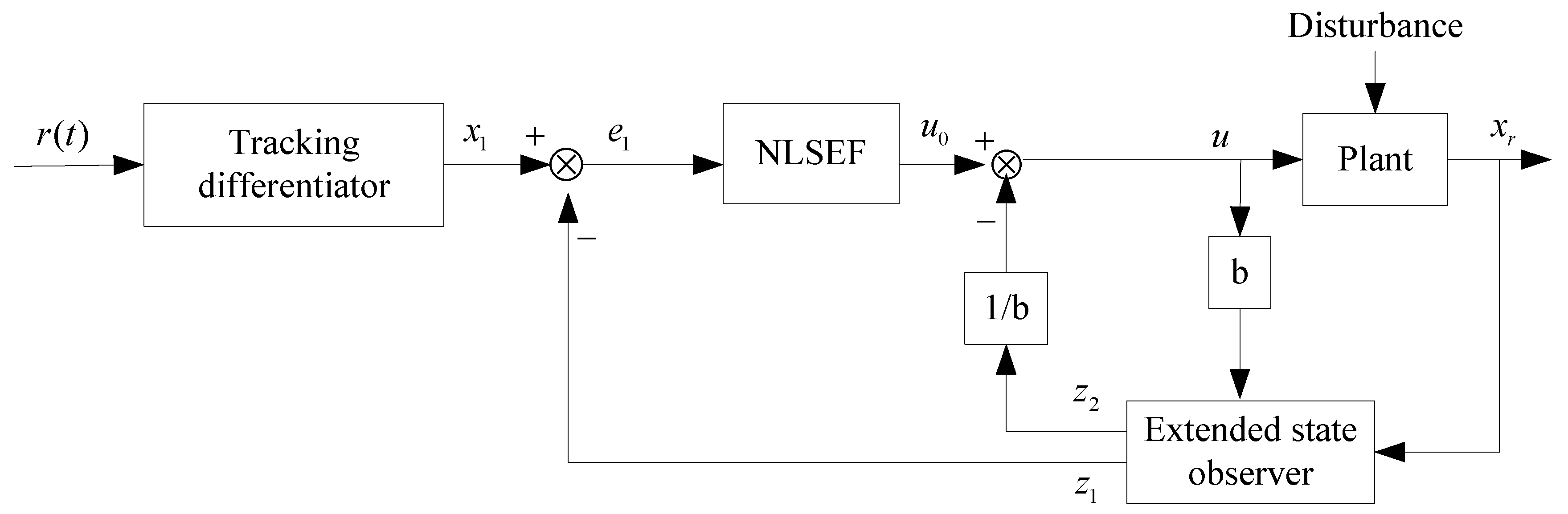
3. Principle of the ADRC

The ADRC offers a new and inherently robust controller that requires very little information of the plant, as shown in Figure 2. It is composed of a tracking differentiator (TD), an extended state observer, and a nonlinear PD controller. For the sake of simplicity, the plant described by the first-order differential equation of Equation (13) is used as the theme problem to illustrate the ADRC-based control design.

$$\{\begin{array}{l}\dot{x}=f\left(x,w,t\right)+b·u\\ y=x\end{array}$$

(13)

where $y$ is the output, $u$ is the input signal, $x$ is the state variable, $w$ denotes external disturbances, $b$ is the system parameter, and $f\left(x,w,t\right)$ is a multivariable function of the state, external disturbance, and time.

3.1. Tracking differentiator (TD)

The tracking differentiator (TD) can quickly track the input signal without set point jump by constructing a transient profile that the output of the plant can reasonably follow, and generate an approximate differential signal of the input signal. The discrete equation is:

$$\{\begin{array}{c}{x}_1\left(t+1\right)=x_1\left(t\right)+T_s{x}_2\left(t\right)\\ x_2\left(t+1\right)=x_2\left(t\right)+T_s·fst\left(x_1\left(t\right)-r\left(t\right),x_2\left(t\right),r,h\right)\end{array}$$

(14)

where $r\left(t\right)$ is the reference input signal of the ADRC. $x_1\left(t\right)$ tracks the input signal $r\left(t\right)$ and $x_2\left(t\right)$ is the first-order derivative of $x_1\left(t\right)$. $T_s$ is the discrete control period. The dynamic performance of the TD can be tuned by $r$ and $h$. $h$ is the filtering parameter. A larger $h$ means a better filtering effect on noise. $r$ determines the tracking effect. The larger the value of $r$, the faster the tracking speed and the greater the overshooting. Therefore, both parameters need to be designed according to the output profile of the TD. The optimal control function of the discrete time system is as follows:

$$fst\left(x_1\left(t\right)-r\left(t\right),x_2\left(t\right),r,h\right)=-\{\begin{array}{c}r·a/d,\hspace{1em}\left|a\right|\le d,\hspace{1em}d=r·h\\ r·sign\left(a\right),\hspace{1em}\left|a\right|>d,\hspace{1em}d=r·h\end{array}$$

(15)

$$a=\{\begin{array}{l}{x}_2\left(t\right)+\frac{a_0-d}{2}·sign\left(e_r\left(t\right)\right),\hspace{1em}\left|e_r\left(t\right)\right|>d_0,\hspace{1em}{d}_0=d·h\\ x_2\left(t\right)+\frac{e_r\left(t\right)}{2},\hspace{1em}\left|e_r\left(t\right)\right|\le d_0,\hspace{1em}{d}_0=d·h\end{array}$$

(16)

$$a_0=\sqrt{d^2+8·r·\left|y\left(t\right)\right|}$$

(17)

$$e_r\left(t\right)=x_1\left(t\right)-r\left(t\right)+h·x_2\left(t\right)$$

(18)

3.2. Extended State Observer (ESO)

Considering $w$ in Equation (13) as a disturbance, a second-order extended state observer can be proposed as:

$$\{\begin{array}{l}e\left(t\right)=z_1\left(t\right)-x_r\left(t\right)\\ z_1\left(t+1\right)=z_1\left(t\right)+T_s·\left[z_2\left(t\right)-{\beta }_{01}·fal\left(e\left(t\right),{\alpha }_1,{\delta }_1\right)+b·u\left(t\right)\right]\\ z_2\left(t+1\right)=z_2\left(t\right)-T_s·{\beta }_{02}·fal\left(e\left(t\right),{\alpha }_1,{\delta }_1\right)\end{array}$$

(19)

where $x_r\left(t\right)$ is the actual feedback signal of the state variable $x\left(t\right)$; $z_1\left(t\right)$ is the estimate of the state variable; $e\left(t\right)$ is the estimation error of the observer; $z_2\left(t\right)$ is the estimation of the total disturbance of the system; and $a_1$, ${\delta }_1$, ${\beta }_{01}$, ${\beta }_{02}$ are four adjustable parameters in the ESO. Taking $0<a_1<1$ for instance, the smaller the value of $a_1$, the stronger the nonlinearity of function $fal\left(e\left(t\right),a_1,{\delta }_1\right)$. This means that the ESO has better resistance to system disturbances. ${\delta }_1$ is the filter parameter of the ESO. ${\beta }_{01}$ and ${\beta }_{02}$ greatly affect the dynamic performance of the system. The estimation of state variables is mainly influenced by ${\beta }_{01}$. The estimation of system disturbance is mainly affected by ${\beta }_{02}$. The larger the values of ${\beta }_{01}$ and ${\beta }_{02}$, the faster the convergence is estimated. However, if they are too large, the output of the ESO might produce an oscillating divergence and a high frequency noise signal. With a well behaved observer, $z_1\left(t\right)$ will closely track the state variable of the system $x_r\left(t\right)$, and $z_2\left(t\right)$ can estimate the total disturbances $f\left(x,w,t\right)$ accurately enough. A nonlinear combination function $fal\left(e\left(t\right),a_1,{\delta }_1\right)$ is:

$$fal\left(e\left(t\right),a_1,{\delta }_1\right)=\{\begin{array}{l}{\left|e\left(t\right)\right|}^{a_1}·sign\left(e\left(t\right)\right),\hspace{1em}\left|e\left(t\right)\right|>{\delta }_1\\ e\left(t\right)·{\delta }_1^{a_1-1},\hspace{1em}\left|e\left(t\right)\right|\le {\delta }_1\end{array}$$

(20)

3.3. Nonlinear State Error Feedback Control Laws (NLSEF)

According to the output of the TD and ESO, the first-order nonlinear state feedback control law is constructed as:

$$\{\begin{array}{l}{e}_1\left(t\right)=x_1\left(t\right)-z_1\left(t\right)\\ u_0\left(t\right)={\beta }_{1}fal\left(e_1\left(t\right),a_{01},{\delta }_{01}\right)\\ u\left(t\right)=u_0\left(t\right)-z_2\left(t\right)/b\end{array}$$

(21)

where $u\left(t\right)$ is the control variable of the ADRC. $a_{01}$, ${\delta }_{01}$, ${\beta }_1$ are adjustable parameters. Their meaning is similar to the adjustable parameters in the ESO.

The ADRC consists of TD, ESO, and NLSEF. According to different application specifications, these three parts can be used separately or in combination.

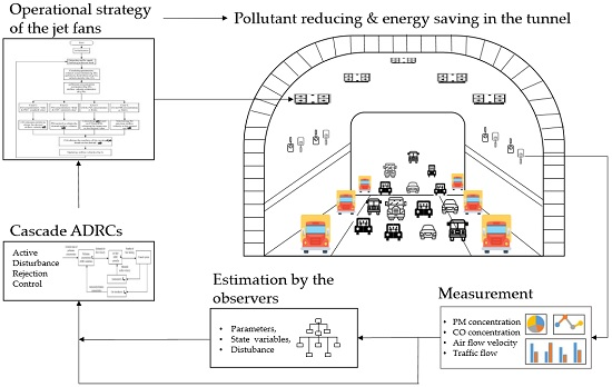
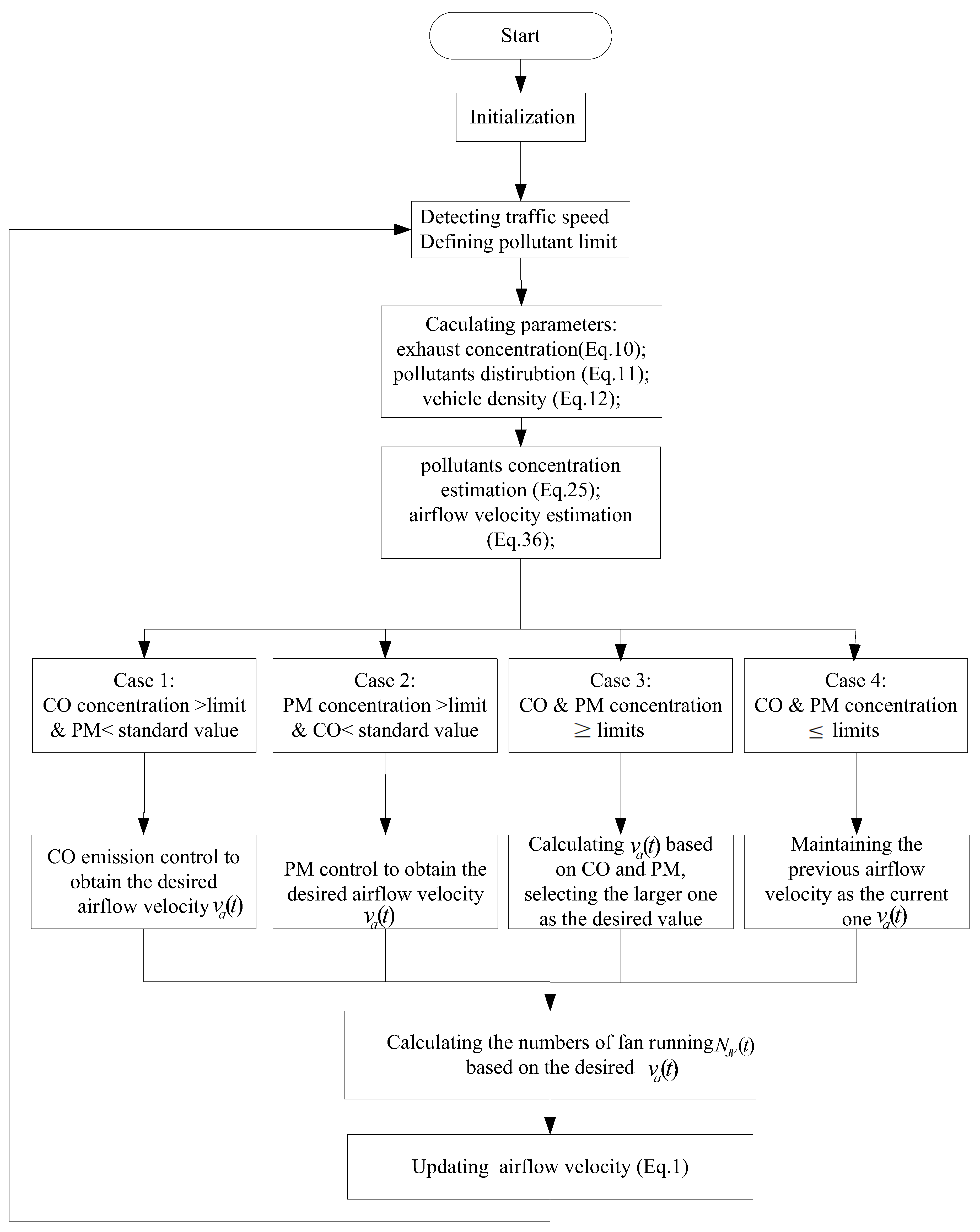
4. Tunnel Ventilation Control System Based on the Active Disturbance Rejection Technique

According to the basic principle of the ADRC, this paper presents a cascade ventilation control system consisting of the pollution control loop and the airflow control loop (Figure 1). The pollution control loop ${\Sigma }_1$ aims to maintain the pollutant concentration below a specified limit. The control variable of airflow control loop ${\Sigma }_2$ is the running number of jet fans. These two control subsystems will be introduced in the following subsections.

4.1. Pollutant Concentration Control Subsystem Based on ADRC

Consider the mass balance equation (Equation (9)) mentioned above; $c\left(x,t\right)$ is a multivariable function of both time and position, and is difficult to mathematically analyze with accuracy. Here, $c\left(x,t\right)$ does not need to be expressively known and can be simplified by the form:

$$\frac{dc}{dt}=f\left(x,t,D,R,b_{0\_c},v_a\right)-b_{0\_c}·v_a$$

(22)

where $b_{0\_c}$ is a certain value, and the remaining uncertainties $\left(b_{0\_c}-\frac{\partial c}{\partial x}\right)·v_a$ are attributed to the total disturbance of the system. This is clearly an ADRC problem and should be treated with Equation (23) taken into account as a total disturbance:

$$f\left(c,x,t,D,R,b_{0\_c},v_a\right)=\frac{dc}{dt}-\frac{\partial c}{\partial t}+\left(b_{0\_c}-\frac{\partial c}{\partial x}\right)v_a+D\frac{{\partial }^{2}c}{\partial x^2}+R$$

(23)

By combining various known and unknown quantities for an overall disturbance, a complex control problem can be converted into a simple one that the ADRC can solve. Since an ADRC controller consists of TD, ESO and NLSEF, the key calculations in line with these can be presented by Equations (24)–(26) accordingly.

$$\{\begin{array}{c}{c}_1\left(t+1\right)=c_1\left(t\right)+T_s·c_2\left(t\right)\\ c_2\left(t+1\right)=c_2\left(t\right)+T_s·fst\left(c_1\left(t\right)-r_c\left(t\right),c_2\left(t\right),r,h\right)\end{array}$$

(24)

where $r_c\left(t\right)$ is the upper limit of the pollutant concentration. $c_1\left(t\right)$ is the concentration estimation and $c_2\left(t\right)$ is the first-order derivative of $c_1\left(t\right)$.

$$\{\begin{array}{l}{e}_c\left(t\right)=z_{1\_c}\left(t\right)-c_r\left(t\right)\\ z_{1\_c}\left(t+1\right)=z_{1\_c}\left(t\right)+T_s·\left[z_{2\_c}\left(t\right)-{\beta }_{01}·fal\left(e\left(t\right),{\alpha }_1,{\delta }_1\right)-b_{0\_c}·v_a\left(t\right)\right]\\ z_{2\_c}\left(t+1\right)=z_{2\_c}\left(t\right)-T_s·{\beta }_{02}·fal\left(e\left(t\right),{\alpha }_1,{\delta }_1\right)\end{array}$$

(25)

where $c_r\left(t\right)$ is the measured pollutant concentration. $z_{1\_c}\left(t\right)$ is the estimation of concentration. $z_{2\_c}\left(t\right)$ is the total disturbance.

$$\{\begin{array}{l}{e}_1\left(t\right)=c_1\left(t\right)-z_{1\_c}\left(t\right)\\ v_a{}_0\left(t\right)={\beta }_{1}fal\left(e_1\left(t\right),a_{01},{\delta }_{01}\right)\\ v_a\left(t\right)=v_a{}_0\left(t\right)+z_{2\_c}\left(t\right)/b_{0\_c}\end{array}$$

(26)

where $v_a\left(t\right)$ is the control variable.

4.2. Airflow Velocity Control Subsystem Based on ADRC

Dynamic behavior of the flow velocity $v_a\left(t\right)$ described by the incompressible non-stationary Bernoulli equation (Equation (2)) can be rewritten by this form:

$$\frac{d{v}_a}{dt}=\Delta P_{pist}-\Delta P_{fric}-\Delta P_{area}-\Delta P_{wind}+\Delta P_{JF\_i}·N_{JV}$$

(27)

$\Delta P_{JF\_i}$ can be represented by the following equation:

$$\{\begin{array}{l}\Delta P_{JF\_i\_1}=k_{JV\_i}·v_{JV\_i}^2·\left(1-\frac{v_r}{v_{JV\_i}}\right)\\ \Delta P_{JF\_i\_2}=k_{JV\_i}·v_{JV\_i}^2·\left(\frac{v_r}{v_{JV\_i}}-\frac{v_a}{v_{JV\_i}}\right)\\ \Delta P_{JF\_i}=\Delta P_{JF\_i\_1}+\Delta P_{JF\_i\_2}\end{array}$$

(28)

where $v_r$ is the maximum airflow velocity. $\Delta P_{JF\_i\_1}$ is the known pressure drop and $\Delta P_{JF\_i\_2}$ refers to the uncertain part of the pressure drop. Similar to the calculation of $\Delta P_{JF\_i}$, $\Delta P_{pist}$, $\Delta P_{fric}$, and $\Delta P_{area}$ can be written as the equations below:

$$\{\begin{array}{l}\Delta P_{pist\_1}=\frac{\rho }{2}·\frac{L}{A_{Tun}·v_{veh}}·\left(v_{veh}-v_r\right)·\left|v_{veh}-v_r\right|·{\gamma }_{conv}·{\displaystyle {\displaystyle \sum }_{i=1}^m}{S}_i·n_i\\ \Delta P_{pist\_2}=\frac{\rho }{2}·\frac{L}{A_{Tun}·v_{veh}}·\left(2·\left(v_{veh}-v_r\right)·\left(v_r-v_a\right)+\left(v_r-v_a\right)·\left|v_r-v_a\right|\right)·{\gamma }_{conv}·{\displaystyle {\displaystyle \sum }_{i=1}^m}{S}_i·n_i\\ \Delta P_{pist}=\Delta P_{pist\_1}+\Delta P_{pist\_2}\end{array}$$

(29)

$$\{\begin{array}{l}\Delta P_{fric\_1}=\frac{\rho }{2}·\lambda ·\frac{L}{D_H}·v_r^2\\ \Delta P_{fric\_2}=\frac{\rho }{2}·\lambda ·\frac{L}{D_H}·\left(v_a^2-v_r^2\right)\\ \Delta P_{fric}=\Delta P_{fric\_1}+\Delta P_{fric\_2}\end{array}$$

(30)

$$\{\begin{array}{l}\Delta P_{area\_1}=\frac{\rho }{2}·\left({\zeta }_{in}+{\zeta }_{out}\right)·v_r^2\\ \Delta P_{area\_2}=\frac{\rho }{2}·\left({\zeta }_{in}+{\zeta }_{out}\right)·\left(v_a^2-v_r^2\right)\\ \Delta P_{area}=\Delta P_{area\_1}+\Delta P_{area\_2}\end{array}$$

(31)

Let

$$f_{air}\left(\Delta P,N_{JV}\right)=\Delta P_{pist\_2}-\Delta P_{fric\_2}-\Delta P_{area\_2}-\Delta P_{wind}+\Delta P_{JF\_i\_2}·N_{JV}$$

(32)

$$b_{1\_air}=\Delta P_{pist\_1}-\Delta P_{fric\_1}-\Delta P_{area\_1}$$

(33)

$$b_{0\_}{}_{air}=\Delta P_{JF\_i\_1}$$

(34)

Therefore, Equation (24) can be rewritten by:

$$\frac{d{v}_a}{dt}=f_{air}\left(\Delta P,N_{JV}\right)+b_{1\_air}+b_{0\_air}·N_{JV}$$

(35)

where $b_{1\_air}$ and $b_{0\_air}$ refer to the model errors which can be regarded as part of the total disturbance. $N_{JV}$ is the control variable. The key parameters in the ESO and NLSEF can be calculated by Equations (36) and (37):

$$\{\begin{array}{l}e\left(t\right)=z_{1\_a}\left(t\right)-v_a{}_r\left(t\right)\\ z_{1\_a}\left(t+1\right)=z_{1\_a}\left(t\right)+T_s·\left[z_{2\_a}\left(t\right)-{\beta }_{01}·fal\left(e\left(t\right),{\alpha }_1,{\delta }_1\right)+b_{1\_air}+b_{0\_air}·N_{JV}\left(t\right)\right]\\ z_{2\_a}\left(t+1\right)=z_{2\_a}\left(t\right)-T_s·{\beta }_{02}·fal\left(e\left(t\right),{\alpha }_1,{\delta }_1\right)\end{array}$$

(36)

where $v_a{}_r\left(t\right)$ is the real airflow velocity measured by anemometers, $z_{1\_a}\left(t\right)$ refers to the state variable, and $z_{2\_a}\left(t\right)$ refers to the estimate of the total disturbances.

$$\{\begin{array}{l}{e}_1\left(t\right)=v_a\left(t\right)-z_{1\_a}\left(t\right)\\ N_{JV0}\left(t\right)={\beta }_{1}fal\left(e_1\left(t\right),a_{01},{\delta }_{01}\right)\\ N_{JV}\left(t\right)=N_{JV0}\left(t\right)-\left[z_{2\_a}\left(t\right)+b_{1\_air}\right]/b_{0\_air}\end{array}$$

(37)

where $v_a\left(t\right)$ is the value of the control variable in Equation (26), which is the reference for this subsystem. By tracking the pollutant concentration curve, the number of running jet fans $N_{JV}\left(t\right)$ can be obtained, and the airflow velocity changed accordingly in a longitudinal ventilation tunnel.

5. Test Results

In this work, a range of tests were performed to optimize the control algorithms and energy consumption.

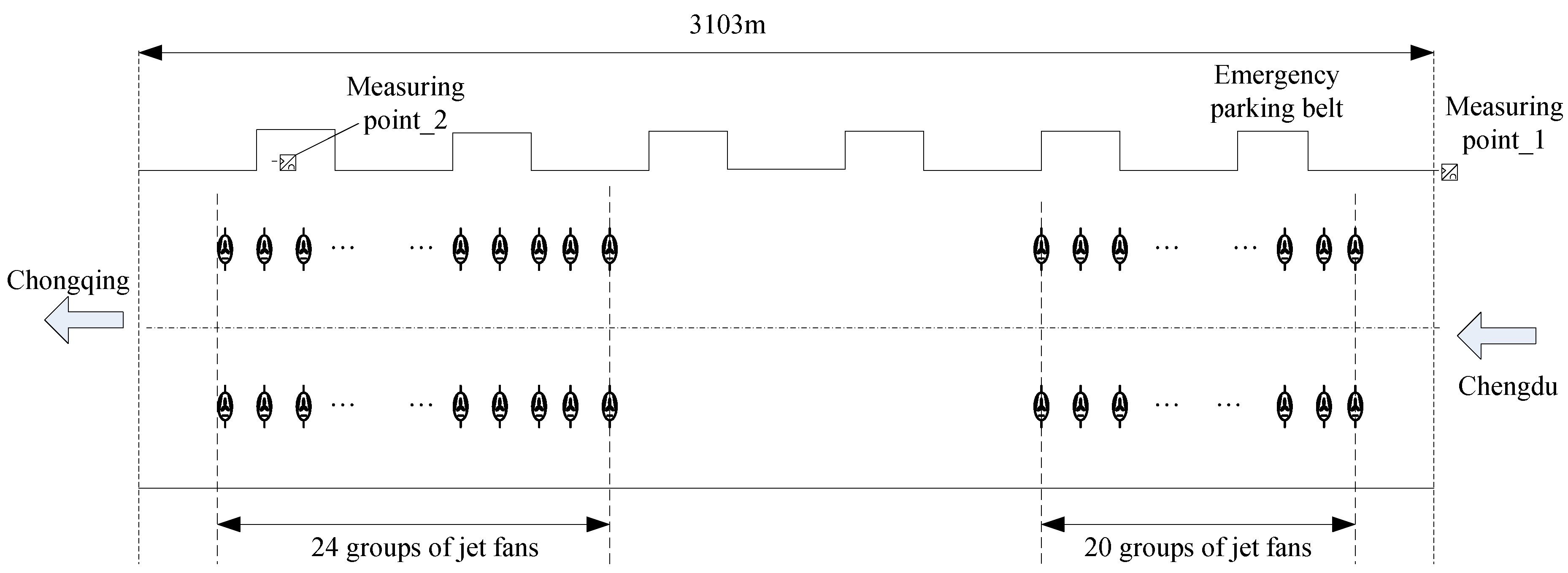
5.1. The Status of the Experimental Tunnel

A ventilation control system based on cascaded ADRC controllers was tested in the simulation model of the right tube of the Zhongliangshan tunnel on the Chengdu–Chongqing expressway in China [24]. Figure 3 shows the layout and installation scheme of the right tube. The parameters of the right tube and vehicle proportion statistics of the peak hours are listed in

Table 1. The parameters of the right tube of the Zhongliangshan tunnel.

Parameter	Value	Parameter	Value	Parameter	Value
$L$/(m)	3103	$A_{Tun}$/(m2)	51.7	$D_H$/(m)	6.44
$\rho$/(kg/m3)	1.156	${\zeta }_{in}$	0.5	${\zeta }_{out}$	1
$\lambda$	0.02	$v_{JV\_i}$/(m/s)	27.5	$A_{JV\_i}$/(m2)	0.63
$K_{e\_i}$	0.7	$N_{JV}$	88

and

Table 2. Vehicle proportion statistics of the peak hours in the right tube of the Zhongliangshan tunnel.

Vehicle Category	Passenger Cars		Truck			Total Amount
	Large	Small	Heavy	Medium	Light
Peak traffic flow (veh/h)	161	1562	257	273	48	2301
Proportion (%)	7	68	11	12	2	100

, respectively.

The test results shown in this section are obtained based on Table 1 and Table 2. If this ADRC scheme is applied to other tunnels or tubes, the parameters will be required to be optimized from measurements to obtain a better model accuracy.

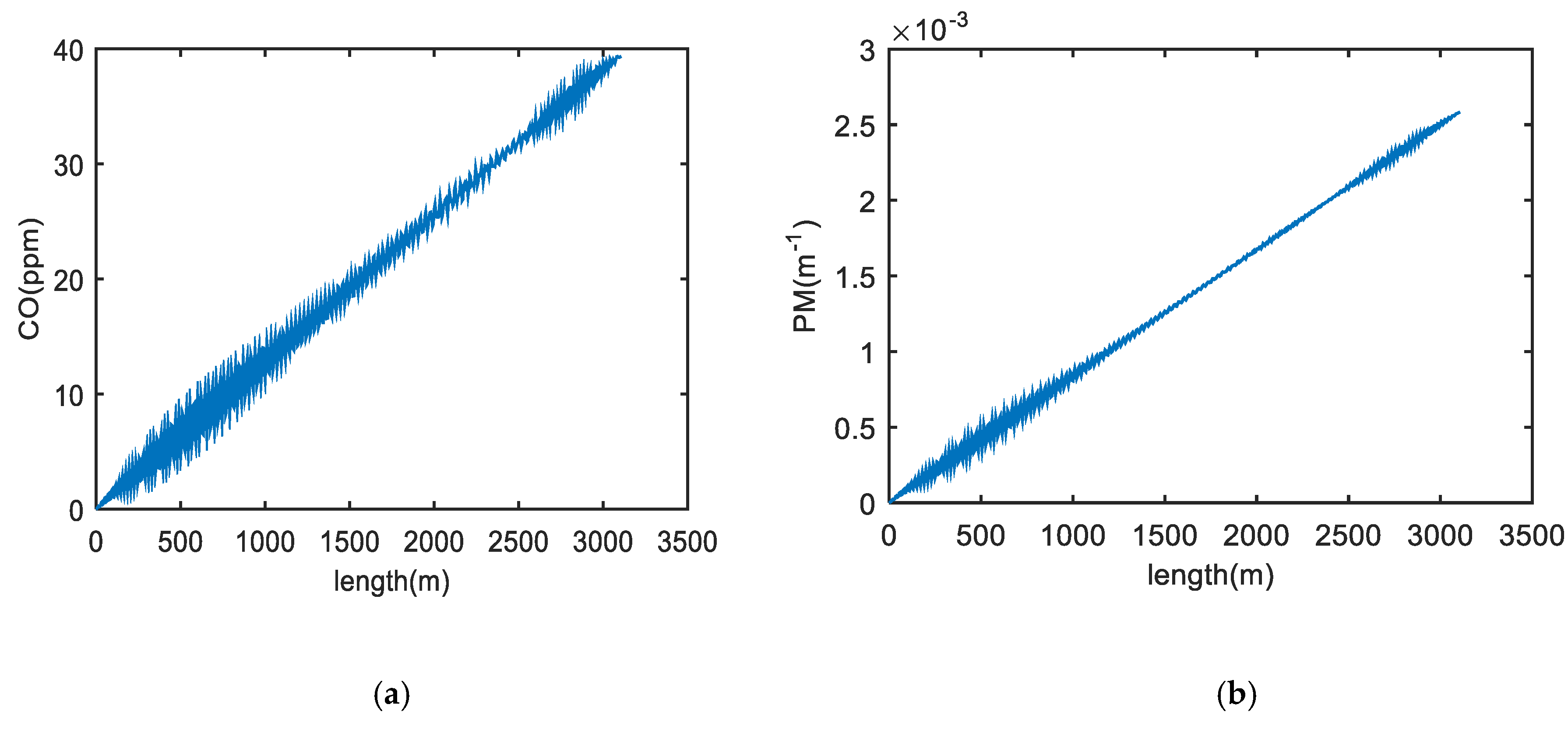
5.2. Effectiveness of the Tunnel Model

The right tube of the experimental tunnel uses a number of jet fans to form a longitudinal ventilation system. Under these circumstances, the concentration of pollutants (CO, PM) increases from the entrance to the exit, and concentration reaches a maximum near the exit. Figure 4 shows that the distribution for CO and PM complies with this change law. These results confirm the effectiveness of the developed model. Moreover, the control result based on this model is also effective, tracking the corresponding changes accordingly.

5.3. The Performance ADRC on Longitudinal Ventilation System

Among the ADRC components, the TD, ESO, and NLSEF can be used separately or together. In order to make full use of the ESO, they start to work by close monitoring CO, PM, and airflow velocity once the system launches. The TD and NLSEF are not activated until the mean concentration of CO or the maximum concentration of PM exceeds the upper limits. A flow chart of operating the system is shown in Figure 5.

The scheme starts with an initialization. Next, the traffic speed is measured and used to define the pollutant concentration limit. Three important elements, namely, the exhaust concentration, pollutant distribution, and vehicle density, are calculated according to Equations (10)–(12). Then, the pollutant concentration and airflow velocity are estimated according to Equations (25) and (36). Four cases of the combination of CO and PM concentration are considered. In each case, the desired airflow is defined accordingly. If CO exceeds the upper limit and PM is lower than the threshold, a desired velocity can be determined by CO emission control by ADRC, and then used. In the following step, the number of running fans is defined as per the desired airflow velocity. Then, the airflow speed is updated. This is a whole loop of the operation.

5.3.1. Performance Analysis of the ESO

Concentration of CO, concentration of PM, and airflow velocity are measured every 15 minutes, and sent to their corresponding ESO. Figure 6 shows that ESO performance is in line with CO concentration in a control period. Figure 6a illustrates the performance of CO concentration observations. The dotted line (estimated value) accurately traces the solid line (actual value) at the value of 20 ppm. Meanwhile, Figure 6b, the total disturbance of the system can be observed ($z_2=229\mathrm{ppm}$). The ESOs for PM concentration and airflow velocity have the same excellent performance.

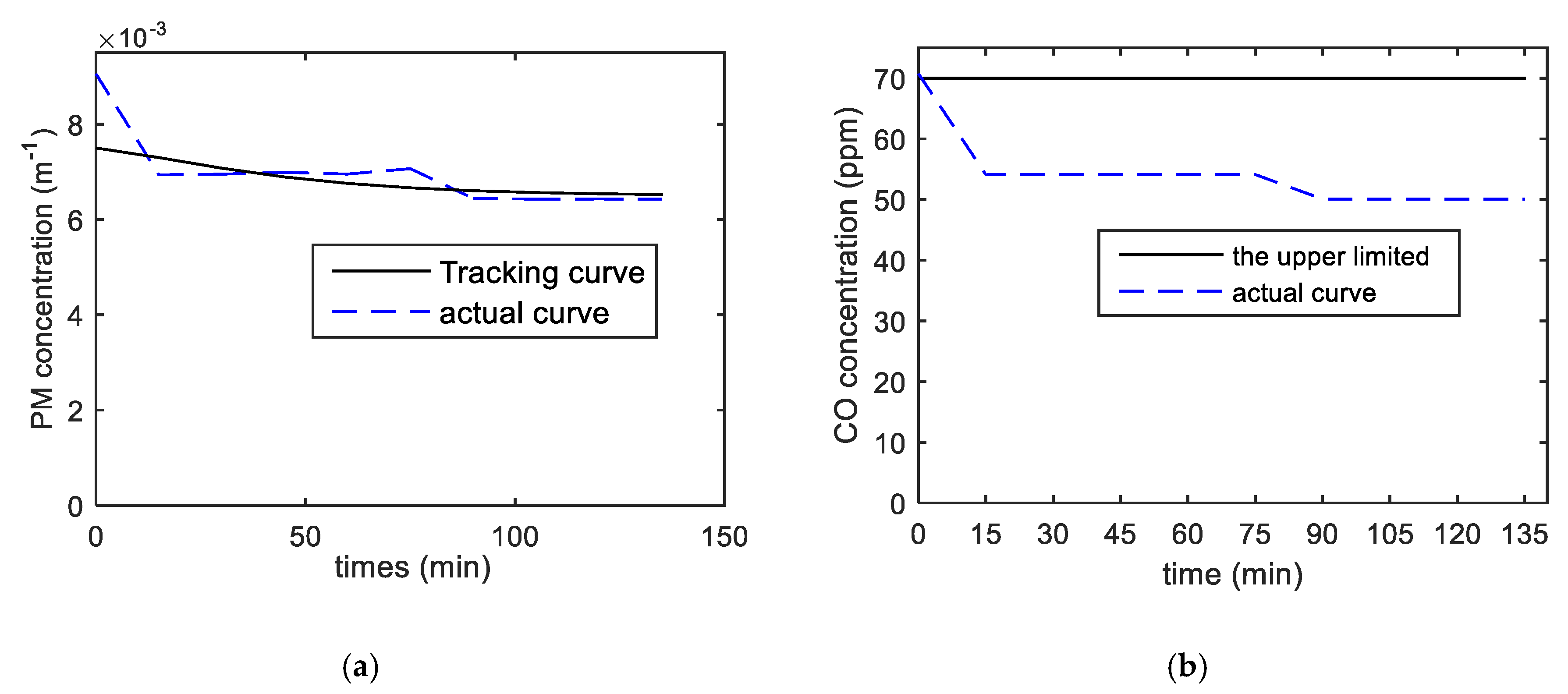
5.3.2. Steady tracking performance

Continuous congestion is used to test the steady tracking performance of the designed control system. When the average speed of the traffic flow drops to 35 km/h, continuous congestion occurs. At this time, the concentrations of CO and PM both exceed the upper limit. The upper limits of the CO and PM concentrations in a congested state are 70 ppm and 0.0075 m⁻¹, respectively. The ADRC controller of CO concentration and PM concentration will give the required airflow velocity. Because the deviation of PM concentration from the upper limit is larger than the deviation of CO concentration, the required wind speed to dilute PM concentration is larger than that required to dilute CO concentration. A larger airflow velocity value than the output reference is selected. The ADRC controller of the air flow velocity will receive the required number of jet fans and then act on it. In order to save the power, it is sufficient that the number of jet fans in operation can reduce the concentration of pollutants to near the upper limits. Therefore, a suitable concentration of PM tracking curve (solid line) is designed in Figure 7a–c, which presents the CO concentration and air flow velocity under control by the proposed method. Figure 7d demonstrates the number of jet fans required.

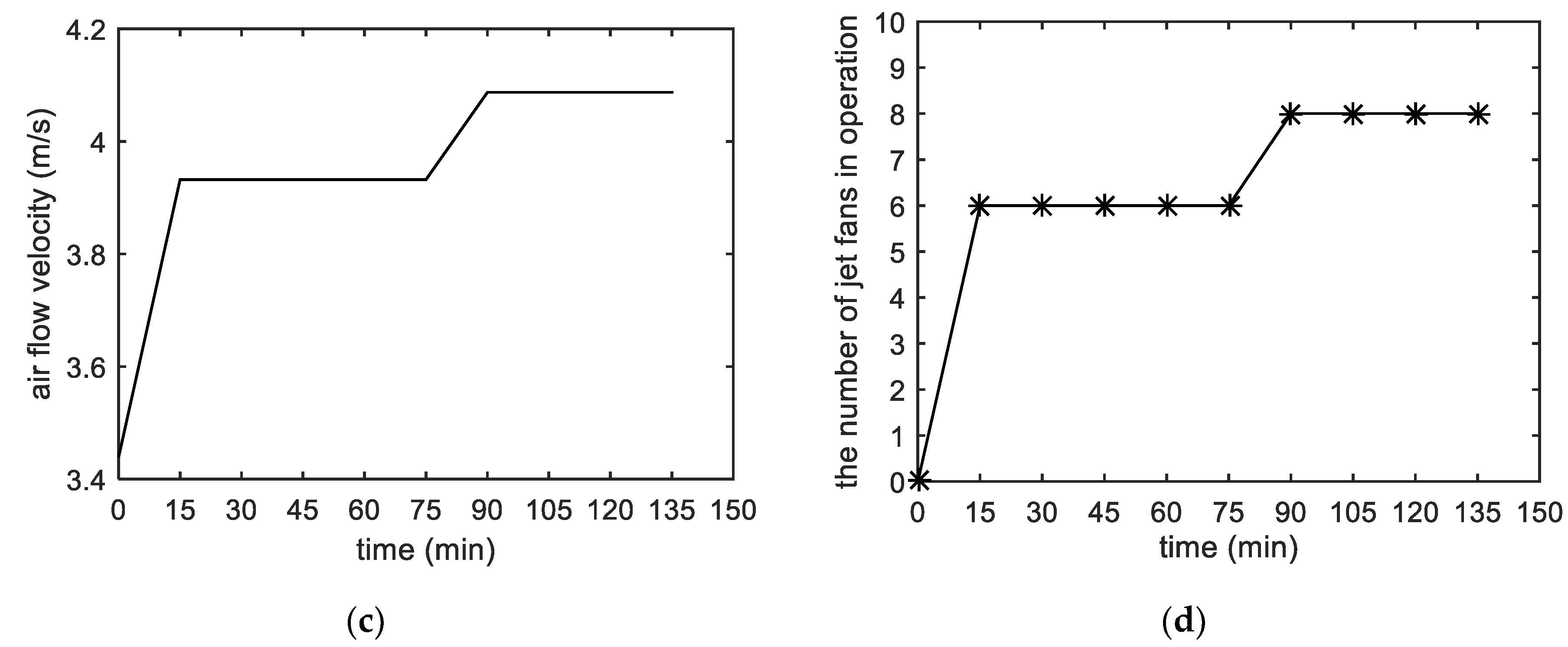
5.3.3. Dynamic Tracking Performance

When the state of traffic flow develops from congestion to stagnation, the concentration of pollutants continues to rise. This process can be used to test the dynamic performance of the designed control system. The upper limits of the CO and PM concentrations in a stagnation state are 70 ppm and 0.009 m⁻¹, respectively. Similar to the congestion state, PM pollutes the air more severely than CO, and is the main control target. This is related to the composition of vehicles in the traffic flow. As can be seen from Table 2, the higher the proportion of diesel heavy vehicles, the larger the amount of PM. Therefore, PM was the main dilution target. The tracking curve is designed as the solid line in Figure 8a. The actual PM concentration curve is shown as the dotted line in Figure 8a. As can be seen, the actual curve is able to track the reference well. The absolute error between the two is less than 0.00079 m⁻¹. Figure 8b reflects the change in CO concentration, which is below the upper limit. Figure 8c,d shows the air speed in the tunnel and the required number of fans running. It can be seen that 10 fans running is needed in ventilation when the traffic is at standstill.

5.3.4. Energy-Saving Performance Analysis

Step control (on-off control) is usually used in ventilation systems [24].

Table 3. Comparison of the step control and the cascade ADRC ventilation control.

Traffic Condition		Normal Traffic (50–100 km/h)	Congestion	Traffic Block $({\mathit{v}}_{\mathit{t}\mathit{r}\mathit{a}\mathit{f}\mathit{f}\mathit{i}\mathit{c}}<30 \mathbf{km}/\mathbf{h})$
Number of jet fans	step control	zero	24 or 48	88
	Cascade ADRC	zero	8	10

shows a comparison of the step control with the proposed method. It can be seen that although step control is simpler and easier to implement, the number of running jet fans is much higher than the cascaded ADRC strategy proposed in this paper. Therefore, the latter can significantly reduce electricity consumption.

6. Conclusions

In this paper, a cascaded longitudinal ventilation control approach based on the ADRC was presented for a road tunnel. This control system consists of a CO and PM concentration control subsystem and an air flow velocity control subsystem. This cascade control method is designed to achieve multiple control objectives. In order to reduce the concentration of pollutants in the tunnel, the forced air flow rate in the tunnel needs to be dynamically controlled. Furthermore, the number of jet fans in operation needs to be optimized to save energy. Therefore, by adopting corresponding control measures for each link, more accurate control schemes can be obtained.

Conventionally, step control is widely used in tunnel ventilation systems. However, this method might cause large fluctuations in the air flow speed over the on/off operation to jet fans, which leads to undesirable dramatic changes in pollutant concentration. By contrast, the proposed ADRC scheme can maintain the pollutant concentration level within a permitted range with minimal energy consumption. The ADRC scheme uses a state observer to capture the external disturbance and compensates for the model uncertainty at the subsystem level to improve the accuracy of the nonlinear control scheme. In this way, the pollutant concentration can be controlled close to the upper limit while running the minimal number of fans. The test results show the effectiveness of the proposed method where the ADRC is used for pollutant control in a tunnel’s longitudinal ventilation in an efficient manner.

However, the ADRC algorithms also have disadvantages. The control algorithms are more complex than step control. Moreover, they include several control parameters in the control loop that are determined by empirical methods based on historical data and trial-and-error. In further work, control parameters will be developed and optimized to improve the system performance. A data-driven method will be utilized to enhance the accuracy of NLSEF for nonlinear problems.

References

1. Funabashi, M.; Aoki, I.; Yahiro, M.; Inoue, H. A fuzzy model based control scheme and its application to a road tunnel ventilation system. In Proceedings of the IECON ‘91: 1991 International Conference on Industrial Electronics, Control and Instrumentation, Kobe, Japan, 28 October–1 November 1991; Volume 2, pp. 1596–1601. [Google Scholar]
2. Koyama, T.; Watanabe, T.; Shinohara, M.; Miyoshi, M.; Ezure, H. Road tunnel ventilation control based on nonlinear programming and fuzzy control. Trans. Inst. Electr. Eng. Jpn. 1993, 113-D, 160–168. [Google Scholar]
3. Chu, B.; Kim, D.; Hong, D.; Park, J.; Chung, J.T.; Chung, J.-H.; Kim, T.-H. GA-based fuzzy controller design for tunnel ventilation systems. Autom. Constr. 2008, 17, 130–136. [Google Scholar] [CrossRef]
4. Bogdan, S.; Birgmajer, B.; Kovačić, Z. Model predictive and fuzzy control of a road tunnel ventilation system. Transp. Res. Part C Emerg. Technol. 2008, 16, 574–592. [Google Scholar] [CrossRef]
5. Euler-Rolle, N.; Fuhrmann, M.; Reinwald, M.; Jakubek, S. Longitudinal tunnel ventilation control. Part 1: Modelling and dynamic feedforward control. Control Eng. Pract. 2017, 63, 91–103. [Google Scholar] [CrossRef]
6. Fuhrmann, M.; Euler-Rolle, N.; Killian, M.; Reinwald, M.; Jakubek, S. Longitudinal tunnel ventilation control. Part 2: Non-linear observation and disturbance rejection. Control Eng. Pract. 2017, 63, 44–56. [Google Scholar] [CrossRef]
7. Roman, R.; Precup, R.; Bojan-Dragos, C.; Szedlak-Stinean, A. Combined model-free adaptive control with fuzzy component by virtual reference feedback tuning for tower crane systems. Procedia Comput. Sci. 2019, 162, 267–274. [Google Scholar] [CrossRef]
8. Kurokawa, R.; Sato, T.; Vilanova, R.; Konishi, Y. Design of optimal PID control with a sensitivity function for resonance phenomenon-involved second-order plus dead-time system. J. Frankl. Inst. 2020, in press. [Google Scholar] [CrossRef]
9. Pilla, R.; Azar, A.T.; Gorripotu, T.S. Impact of flexible AC transmission system devices on automatic generation control with a metaheuristic based fuzzy PID controller. Energies 2019, 12, 4193. [Google Scholar] [CrossRef] [Green Version]
10. Han, J. From PID to active disturbance rejection control. IEEE Trans. Ind. Electron. 2009, 56, 900–906. [Google Scholar] [CrossRef]
11. Sun, B.; Gao, Z. A DSP-based active disturbance rejection control design for a 1-kW H-bridge DC–DC power converter. IEEE Trans. Ind. Electron. 2005, 52, 1271–1277. [Google Scholar] [CrossRef] [Green Version]
12. Lotfi, N.; Zomorodi, H.; Landers, R.G. Active disturbance rejection control for voltage stabilization in open-cathode fuel cells through temperature regulation. Control Eng. Pract. 2016, 56, 92–100. [Google Scholar] [CrossRef]
13. Madonski, R.; Shao, S.; Zhang, H.; Gao, Z.; Yang, J.; Li, S. General error-based active disturbance rejection control for swift industrial implementations. Control Eng. Pract. 2019, 84, 218–229. [Google Scholar] [CrossRef]
14. Su, Y.; Zheng, C.; Duan, B. Automatic disturbances rejection controller for precise motion control of permanent-magnet synchronous motors. IEEE Trans. Ind. Electron. 2005, 52, 814–823. [Google Scholar] [CrossRef]
15. Chu, Z.; Sun, Y.; Wu, C.; Sepehri, N. Active disturbance rejection control applied to automated steering for lane keeping in autonomous vehicles. Control Eng. Pract. 2018, 74, 13–21. [Google Scholar] [CrossRef]
16. Michalek, M.M. Robust trajectory following without availability of the reference time-derivatives in the control scheme with active disturbance rejection. In Proceedings of the 2016 American Control Conference (ACC), Boston, MA, USA, 6–8 July 2016; pp. 1536–1541. [Google Scholar] [CrossRef]
17. Xia, Y.; Shi, P.; Liu, G.P.; Rees, D.; Han, J. Active disturbance rejection control for uncertain multivariable systems with time-delay. IET Control Theory Appl. 2007, 1, 75–81. [Google Scholar] [CrossRef]
18. Madonski, R.; Nowicki, M.; Herman, P. Practical solution to positivity problem in water management systems—An ADRC approach. In Proceedings of the 2016 American Control Conference (ACC), Boston, MA, USA, 6–8 July 2016; pp. 1542–1547. [Google Scholar] [CrossRef]
19. Kurka, L.; Ferkl, L.; Sládek, O.; Porízek, J. Simulation of traffic, ventilation and exhaust in a complex road tunnel. In Proceedings of the 16th IFAC World Congress, Prague, Czechia, 3–8 July 2005; pp. 60–65. [Google Scholar]
20. Ferkl, L.; Meinsma, G. Finding optimal ventilation control for highway tunnels. Tunn. Undergr. Space Technol. 2007, 22, 222–229. [Google Scholar] [CrossRef]
21. Šulc, J.; Ferkl, L.; Cigler, J.; Zápařka, J. Model-based airflow controller design for fire ventilation in road tunnels. Tunn. Undergr. Space Technol. 2016, 60, 121–134. [Google Scholar] [CrossRef]
22. Šulc, J.; Skogestad, S. A systematic approach for airflow velocity control design in road tunnels. Control Eng. Pract. 2017, 69 (Suppl. C), 61–72. [Google Scholar] [CrossRef]
23. JTG/T D70/2-02-2014. Guidelines for Design of Ventilation of Highway Tunnels; Communications Publishing &Media Management Co., Ltd.: Beijing, China, 2014. (In Chinese)
24. Liu, H.; Wang, X.; Chen, J. Test and analysis of Zhongliangshan road tunnel. J. Chongqing Jiaotong Univ. Nat. Sci. 2010, 29, 529–532. (In Chinese) [Google Scholar]
Figure 1. Configuration of a ventilation control system based on the cascade active disturbance rejection control (ADRC).
Energies 13 01871 g001
Figure 2. Block diagram of the ADRC.
Energies 13 01871 g002
Figure 3. The layout and installation scheme of the right tube of the Zhongliangshan tunnel.
Energies 13 01871 g003
Figure 4. Concentration distribution of the pollutants along the tunnel axis: (a) concentration distribution of CO; (b) concentration distribution of particulate matter (PM).
Energies 13 01871 g004
Figure 5. The flow chart of the simulation system.
Energies 13 01871 g005
Figure 6. The results of the extended state observer (ESO) for CO concentration: (a) the observation z 1 (dotted line) and the actual value y r (solid line) of CO concentration; (b) the observations z 2 of the total disturbance.
Energies 13 01871 g006
Figure 7. The steady tracking results of the cascaded ADRC ventilation system at every sample time: (a) PM concentration tracking results; (b) CO concentration; (c) air flow velocity; (d) the number of jet fans in operation.
Energies 13 01871 g007aEnergies 13 01871 g007b
Figure 8. The dynamic tracking results of the cascaded ADRC ventilation system at every sample time: (a) PM concentration tracking results; (b) CO concentration; (c) air flow velocity; (d) the number of jet fans in operation.
Energies 13 01871 g008aEnergies 13 01871 g008b