System Characteristics Analysis for Energy Management of Power-Split Hydraulic Hybrids


Abstract
1. Introduction
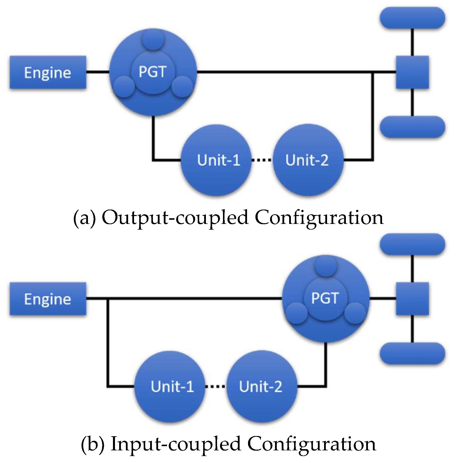
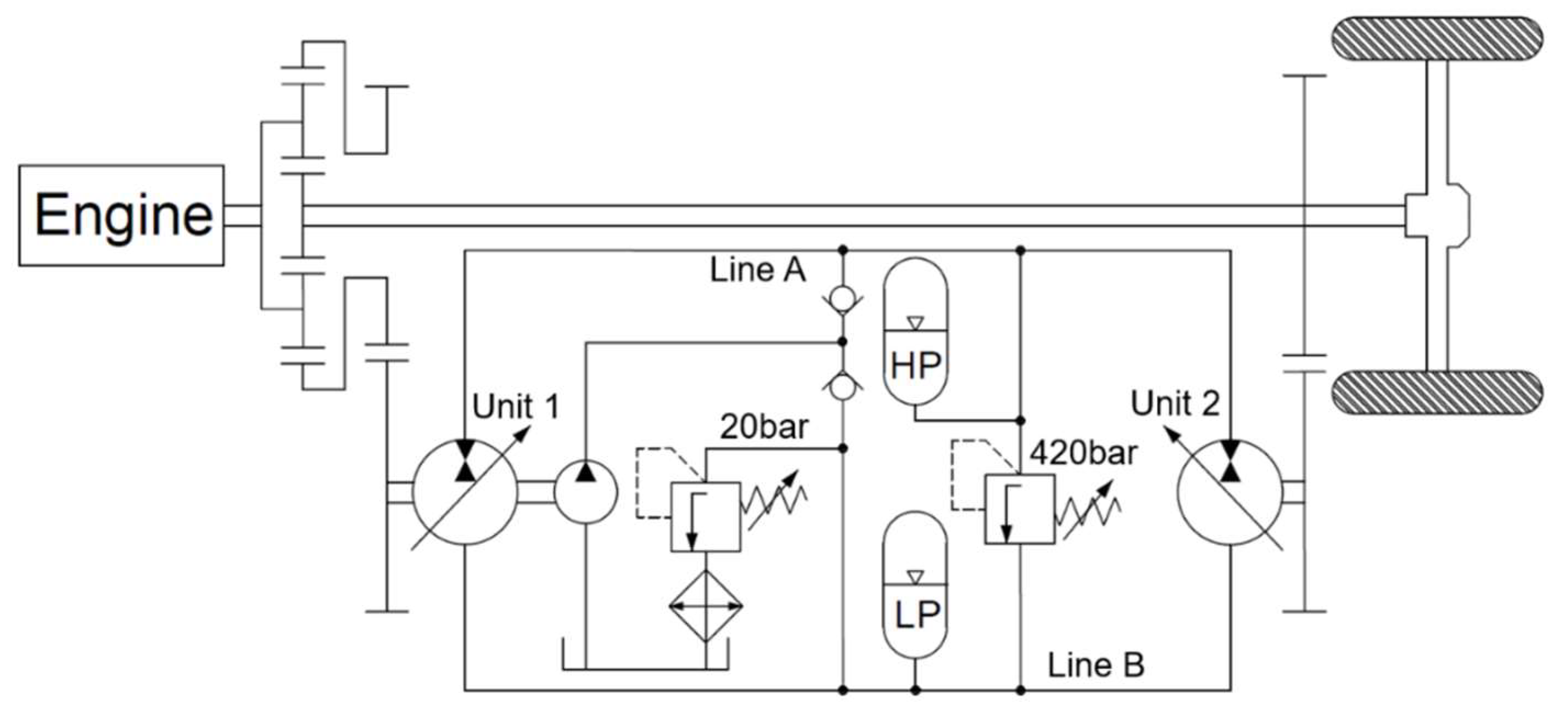
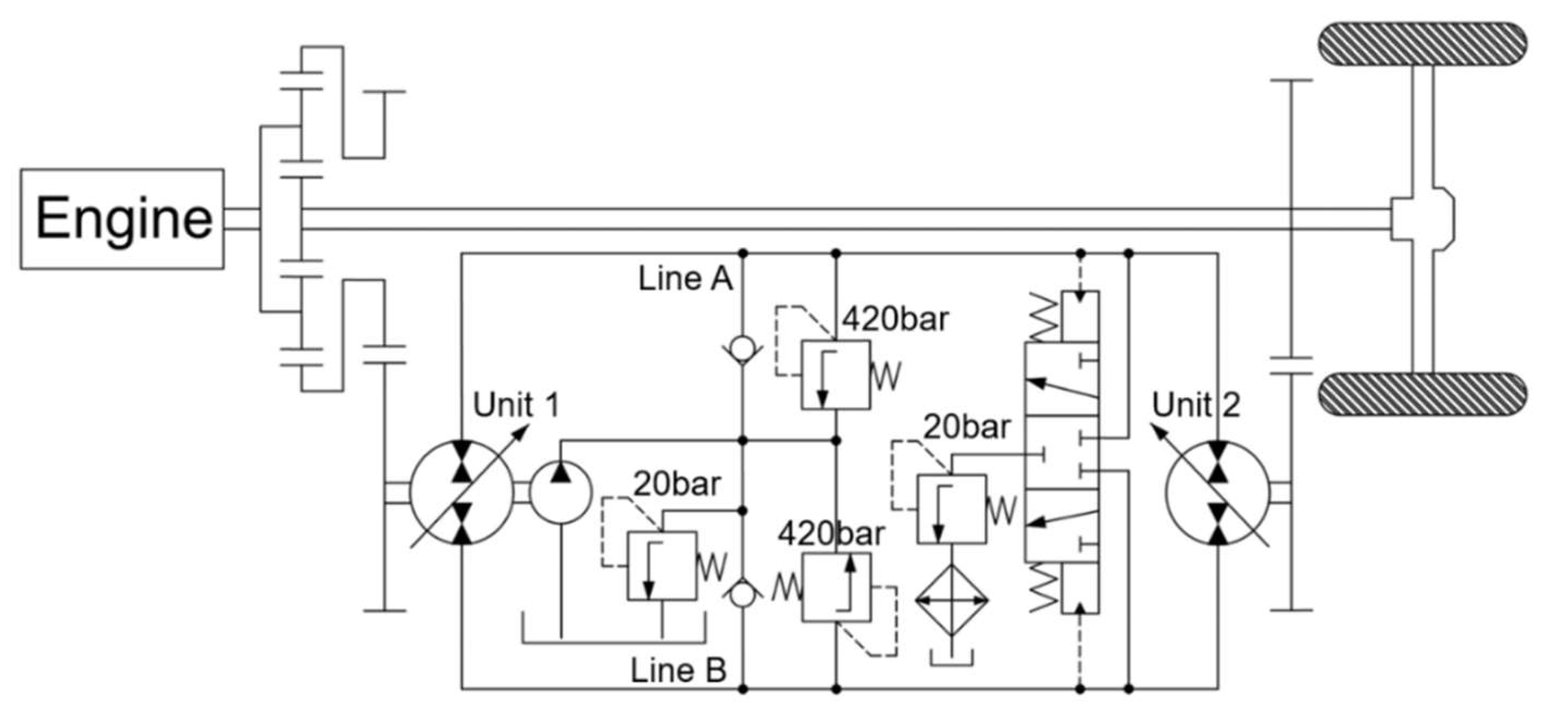
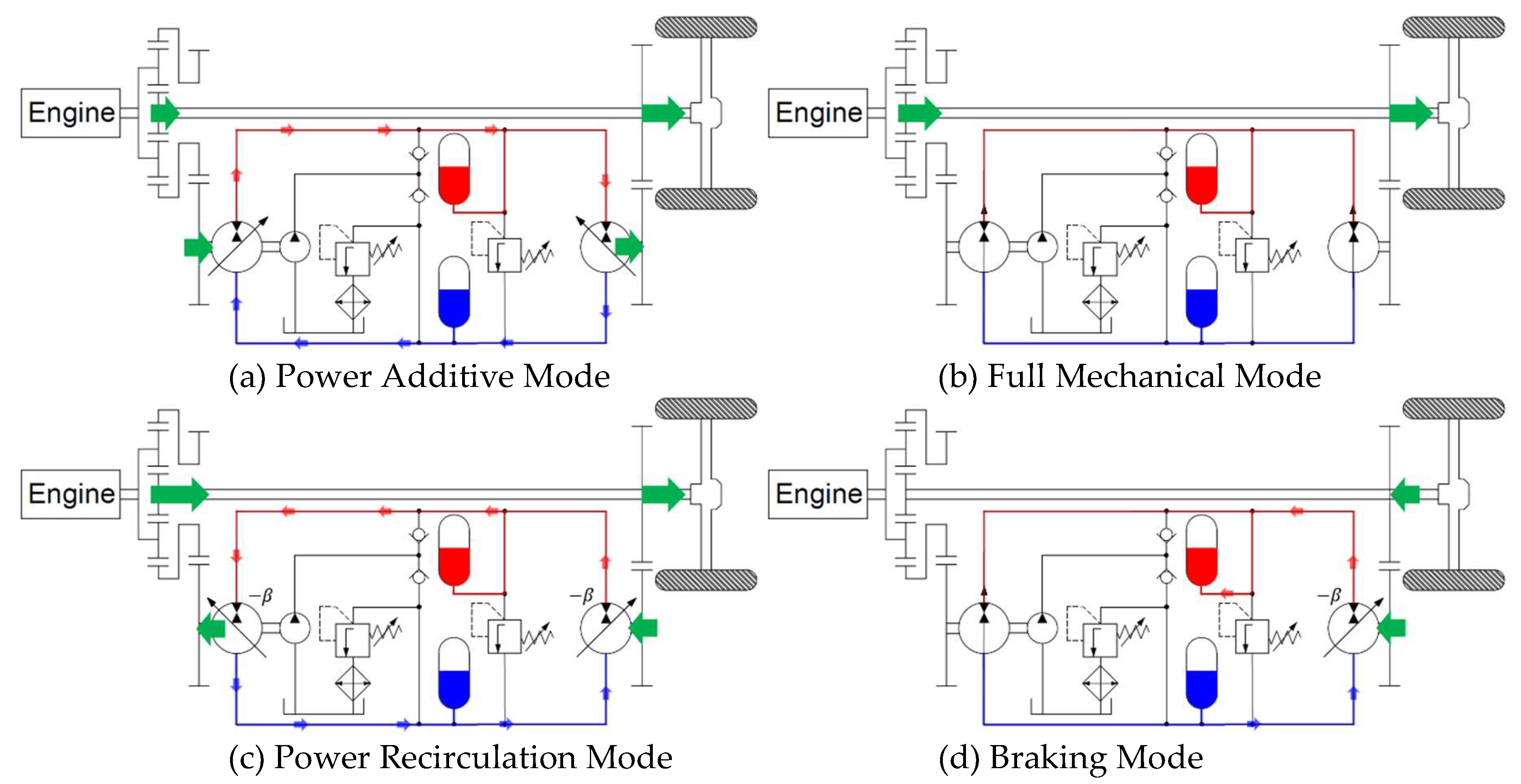
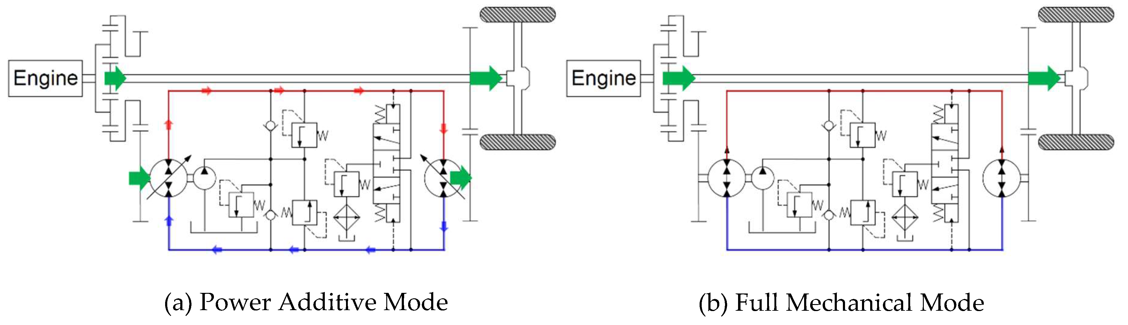
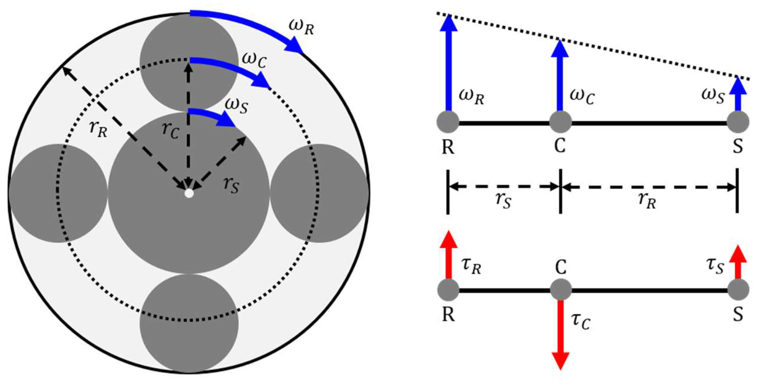
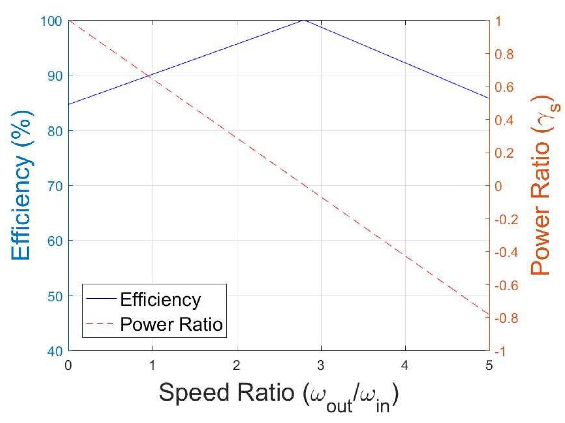
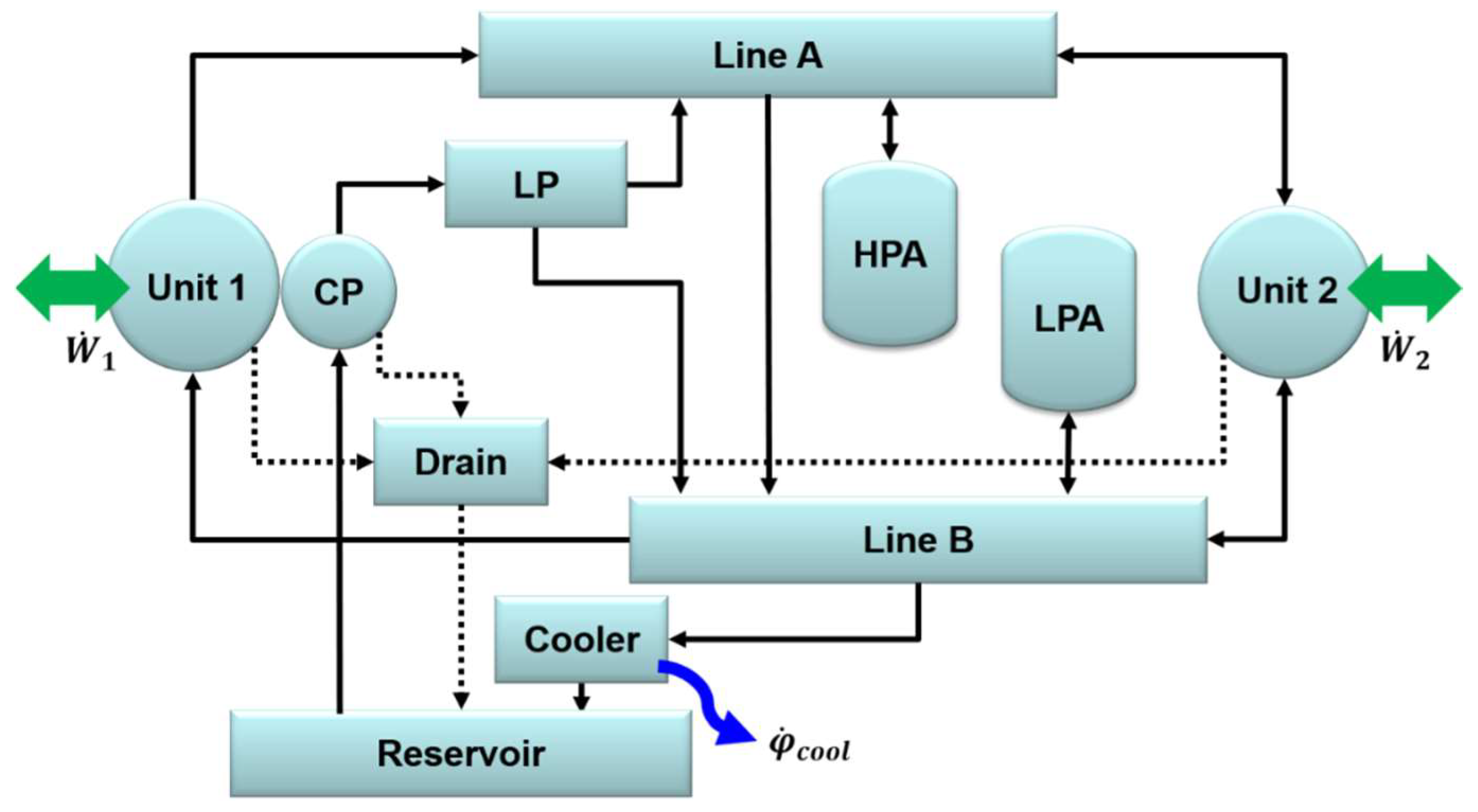
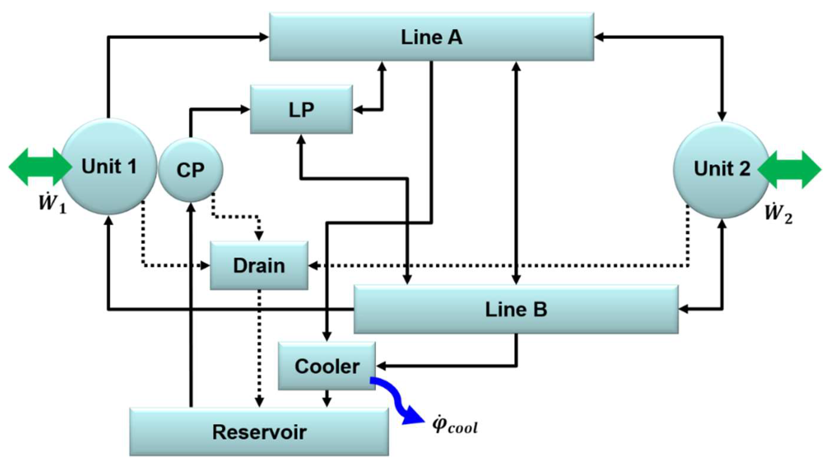
2. System Analysis
3. Numerical Analysis
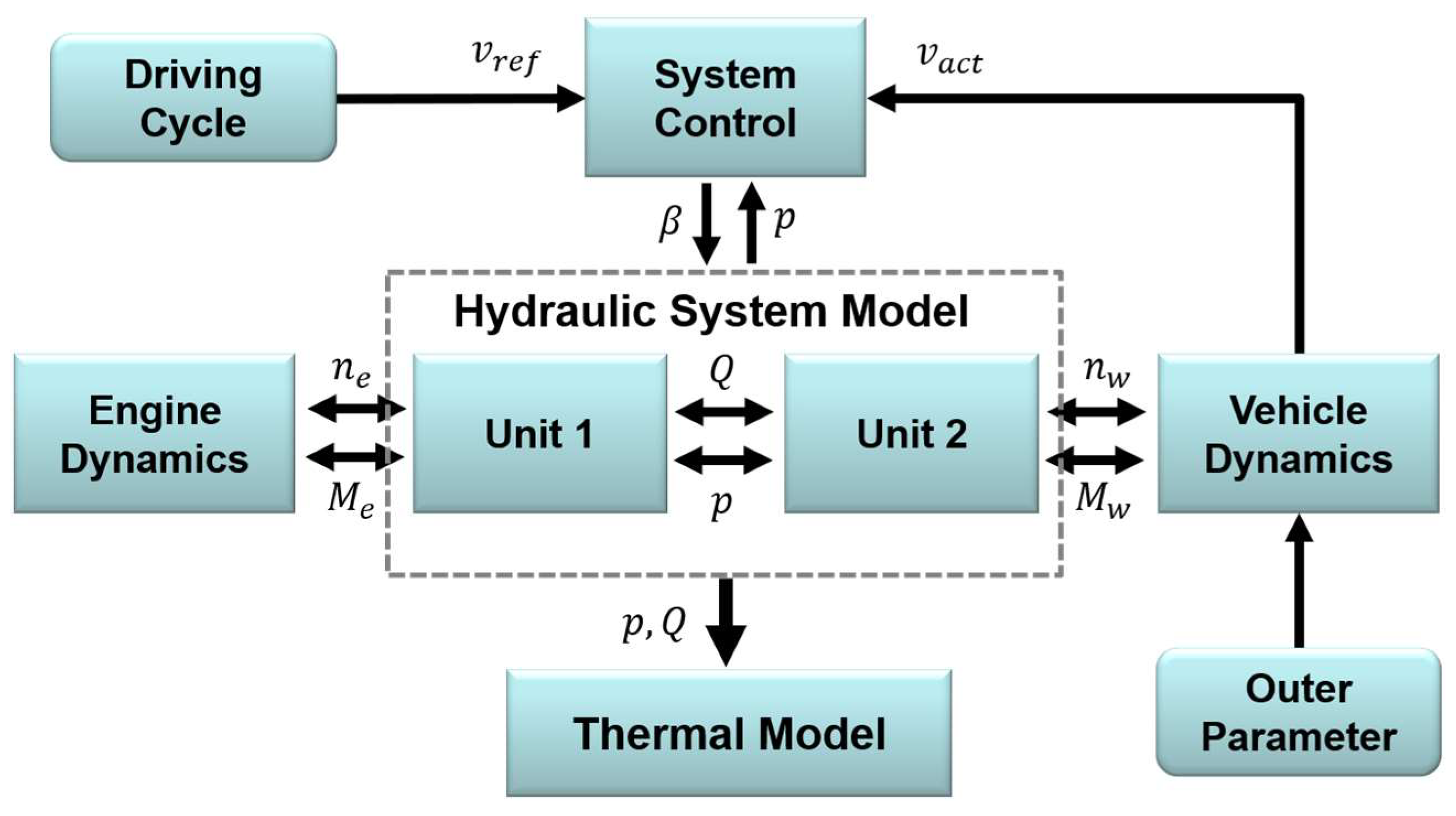
3.1. Modeling Approach
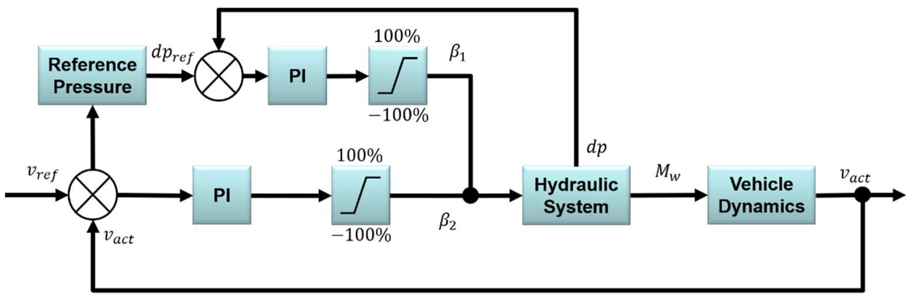
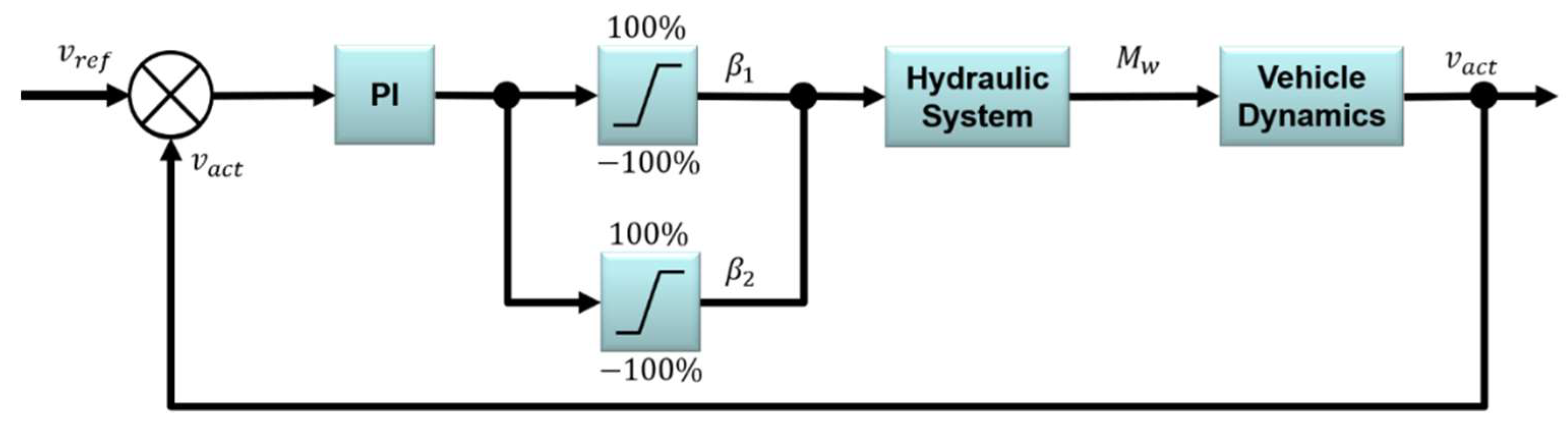
3.2. Dynamic System Modeling
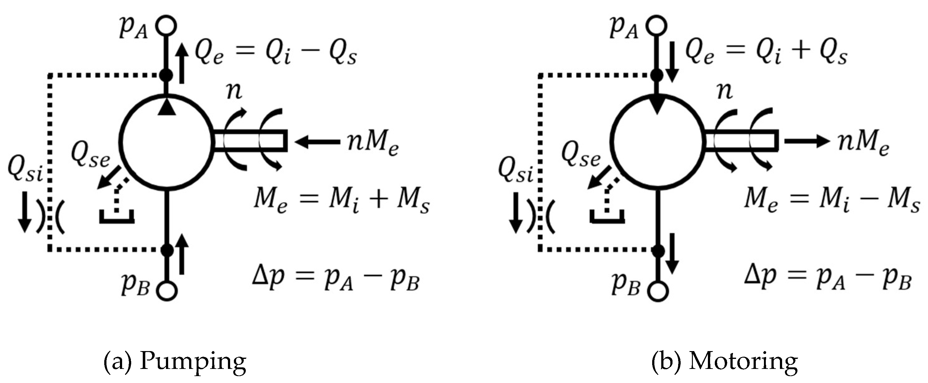
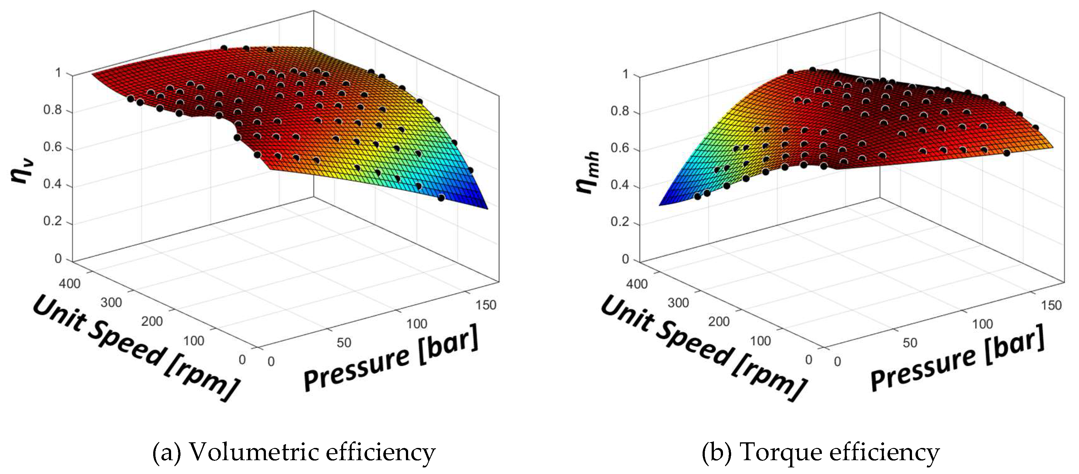
3.3. Hydraulic System Modeling
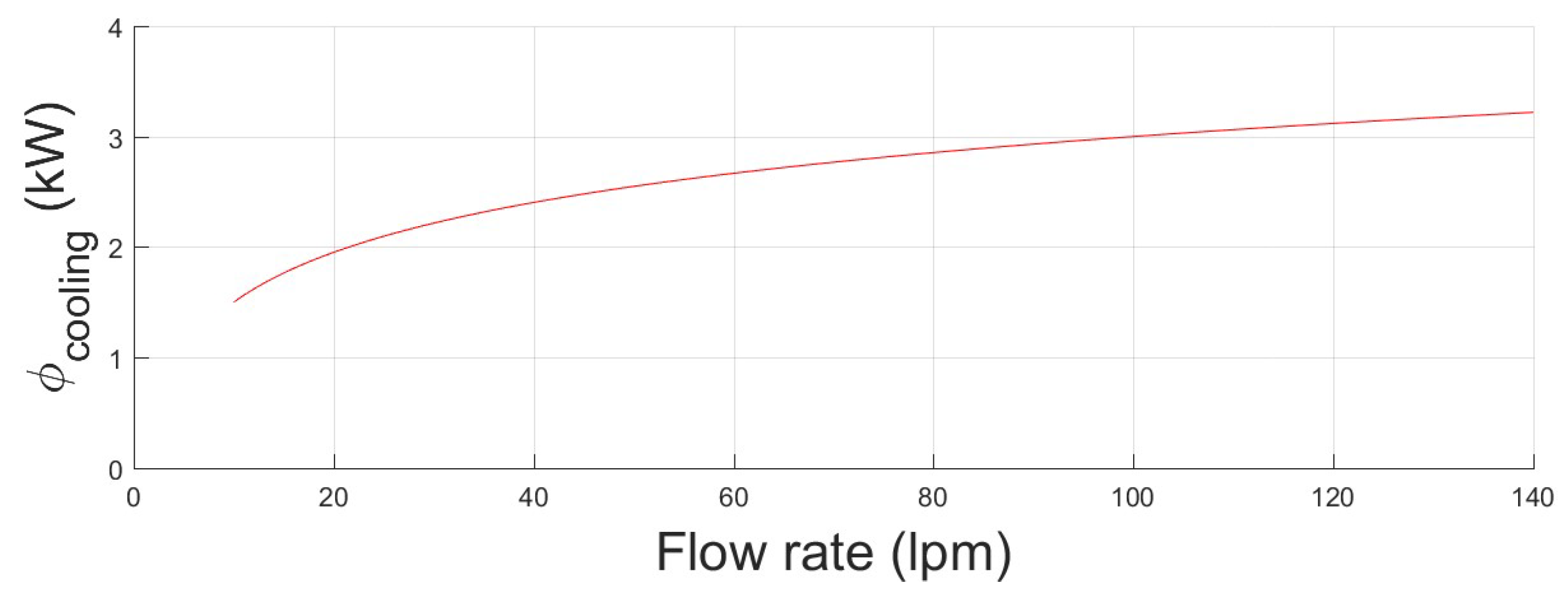
3.4. Thermal Modeling
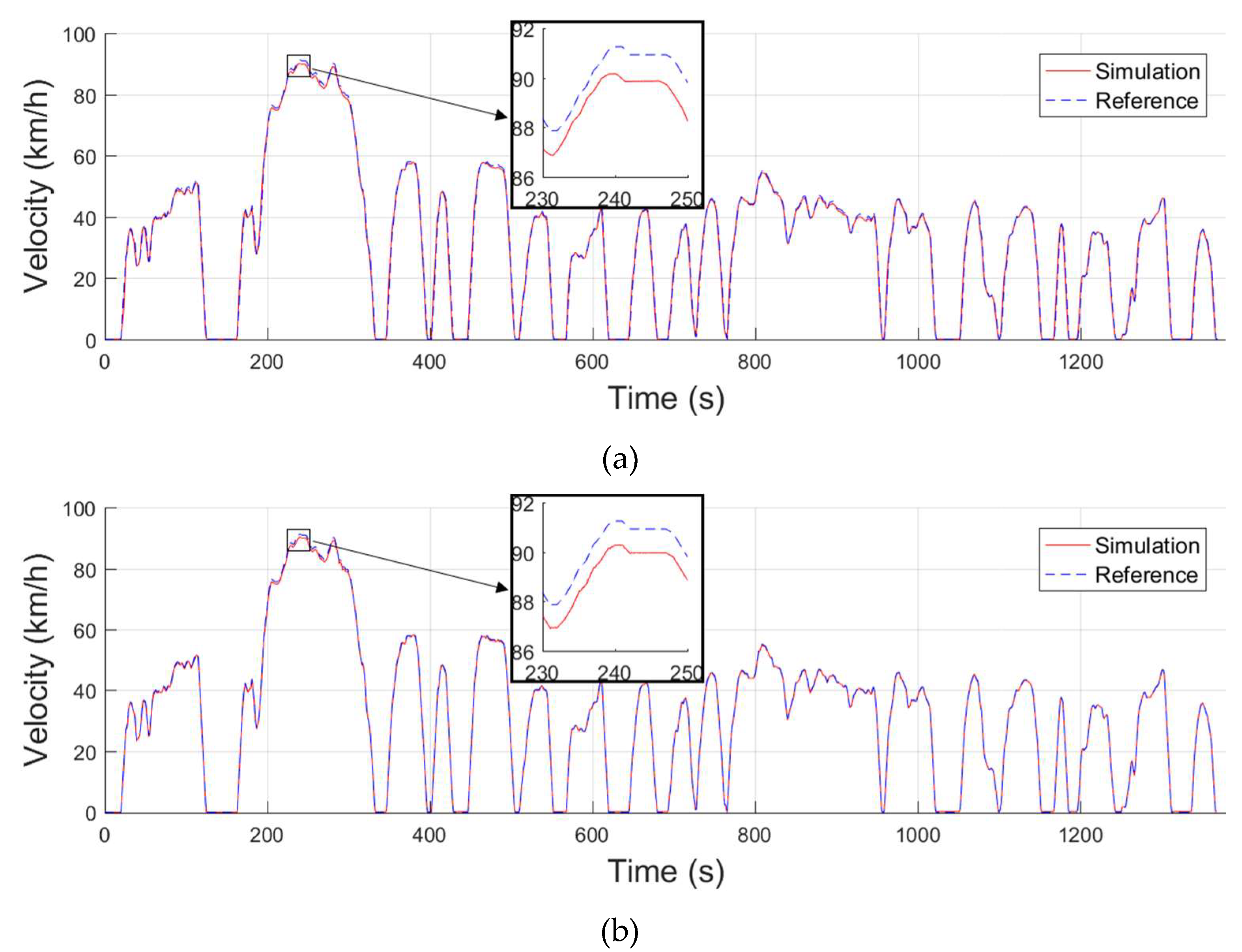
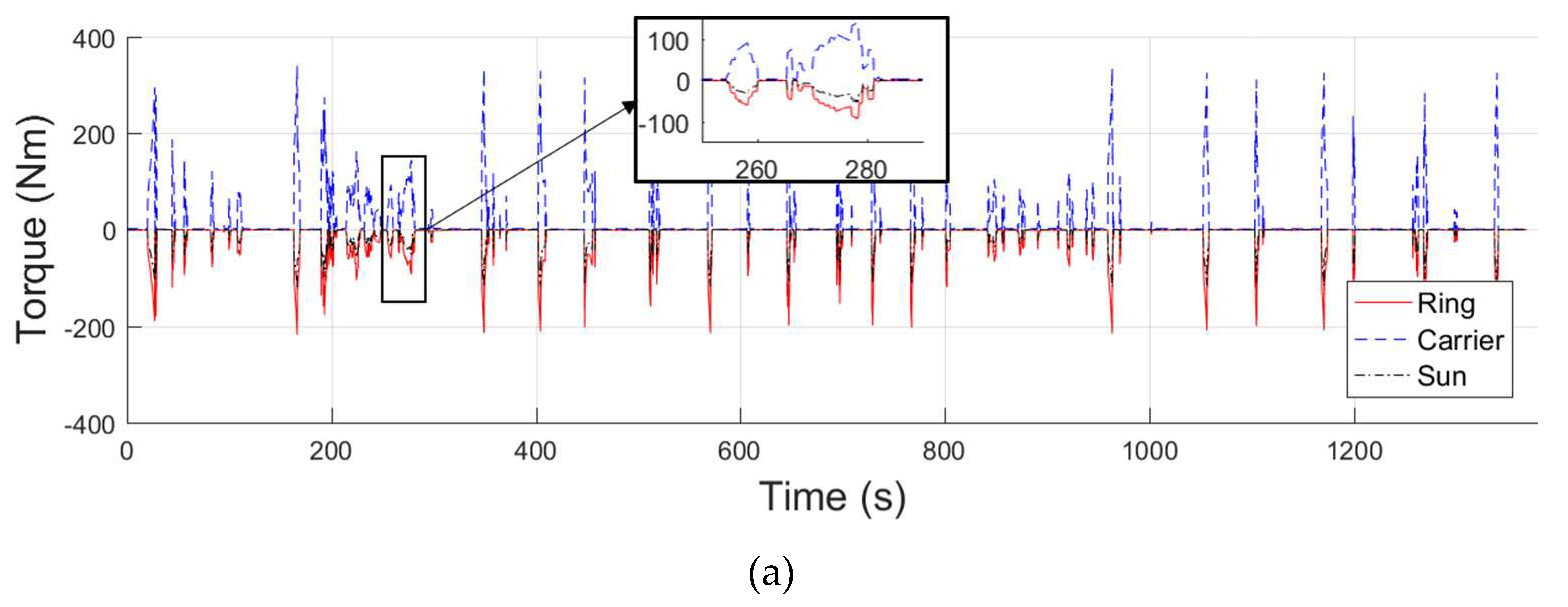
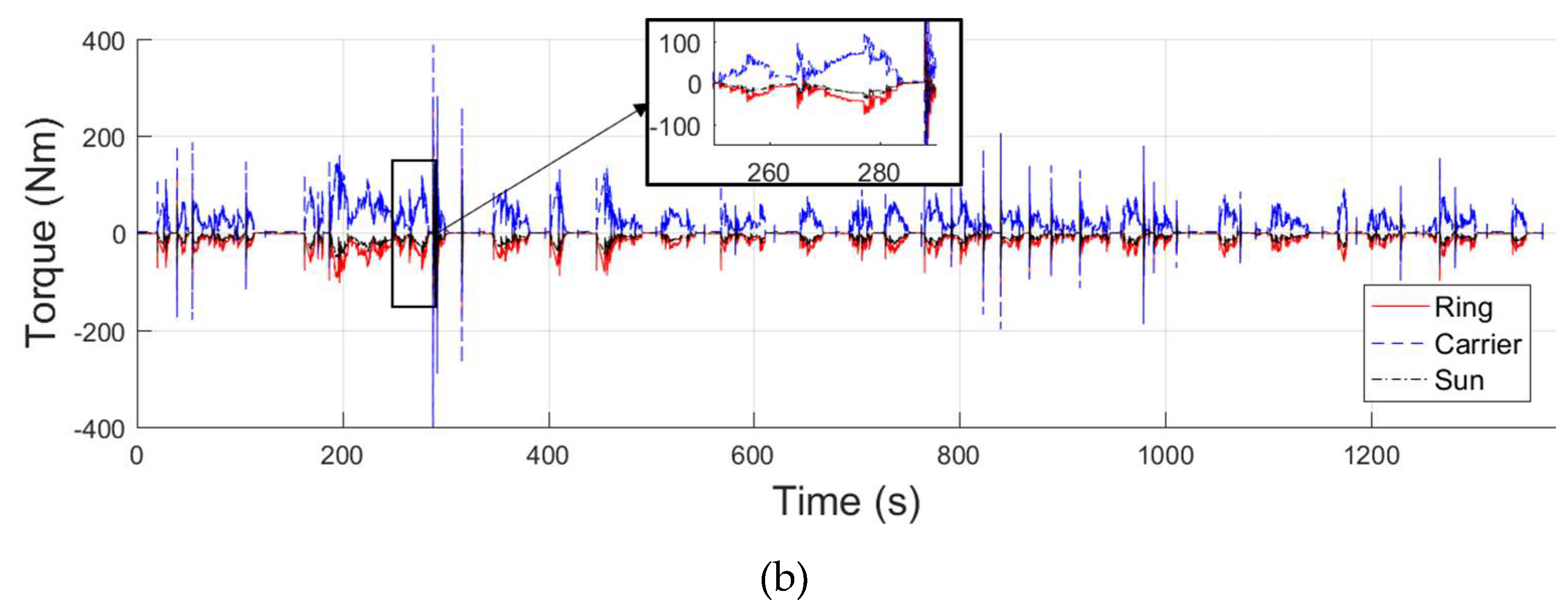
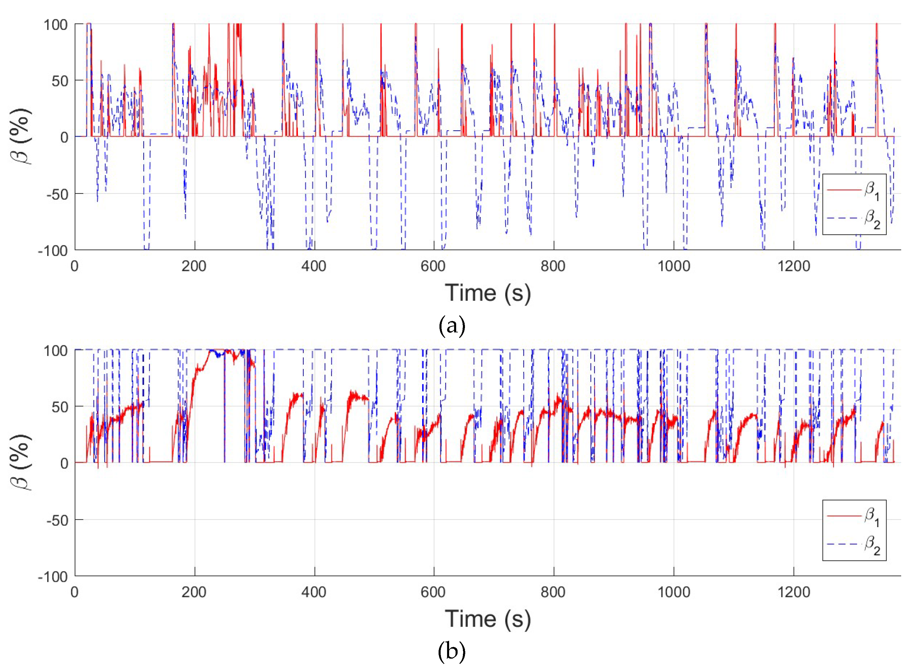
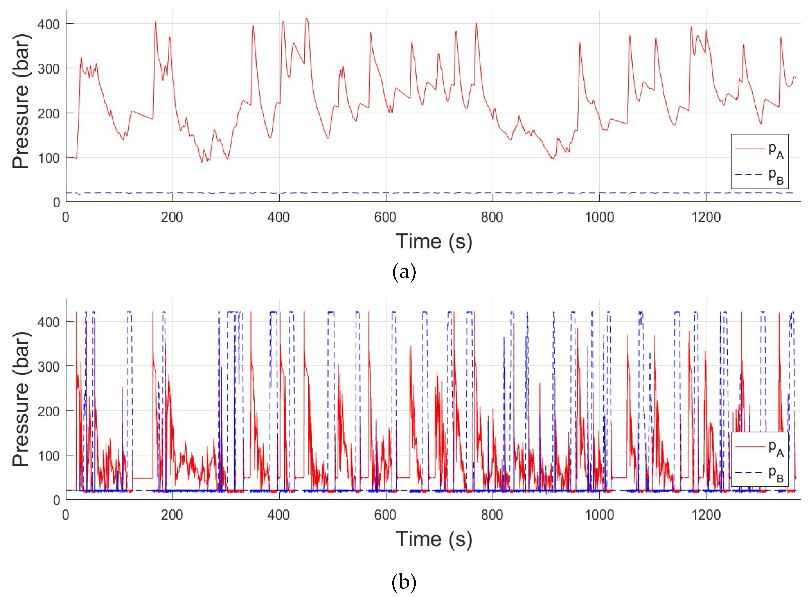
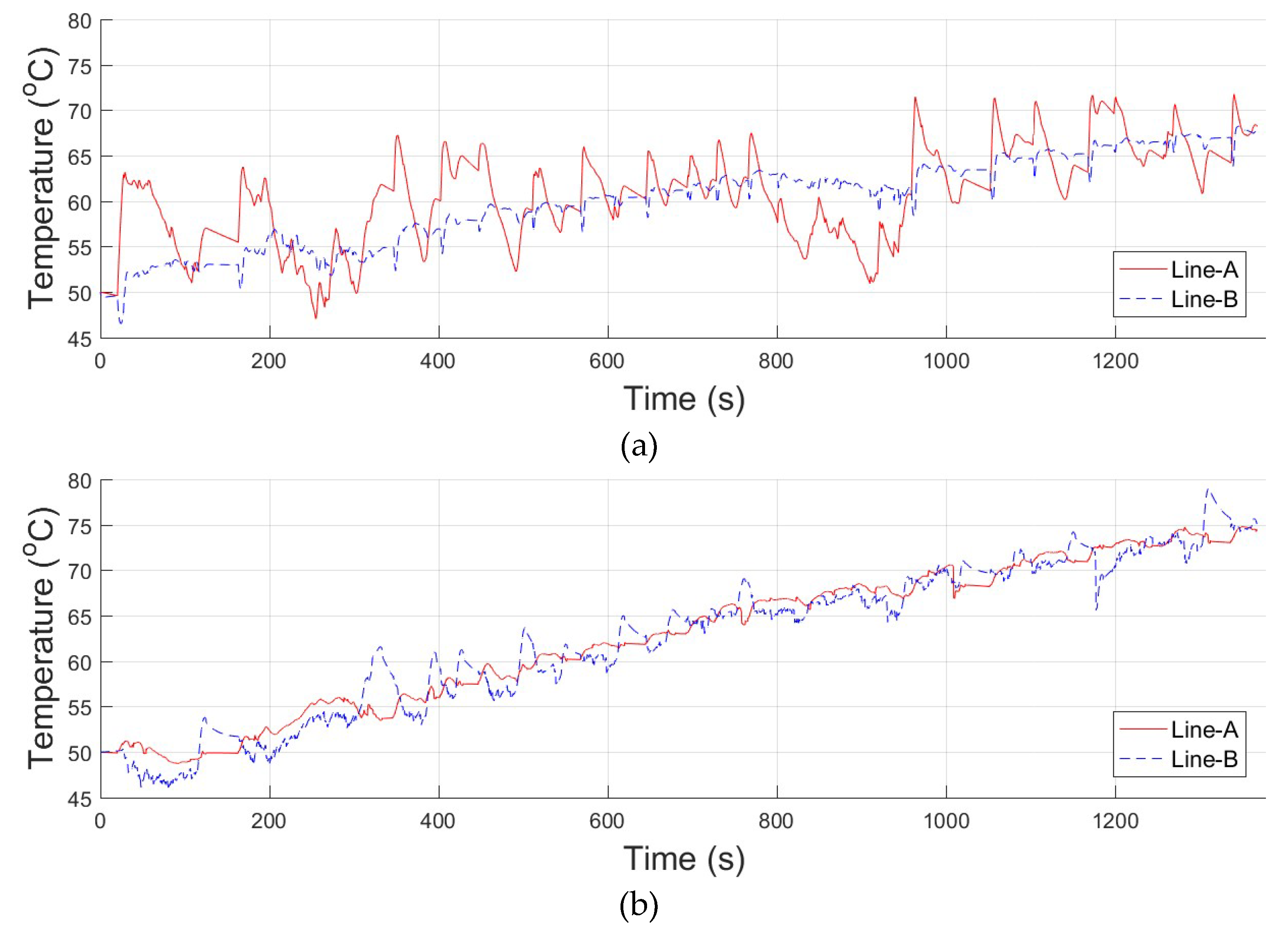
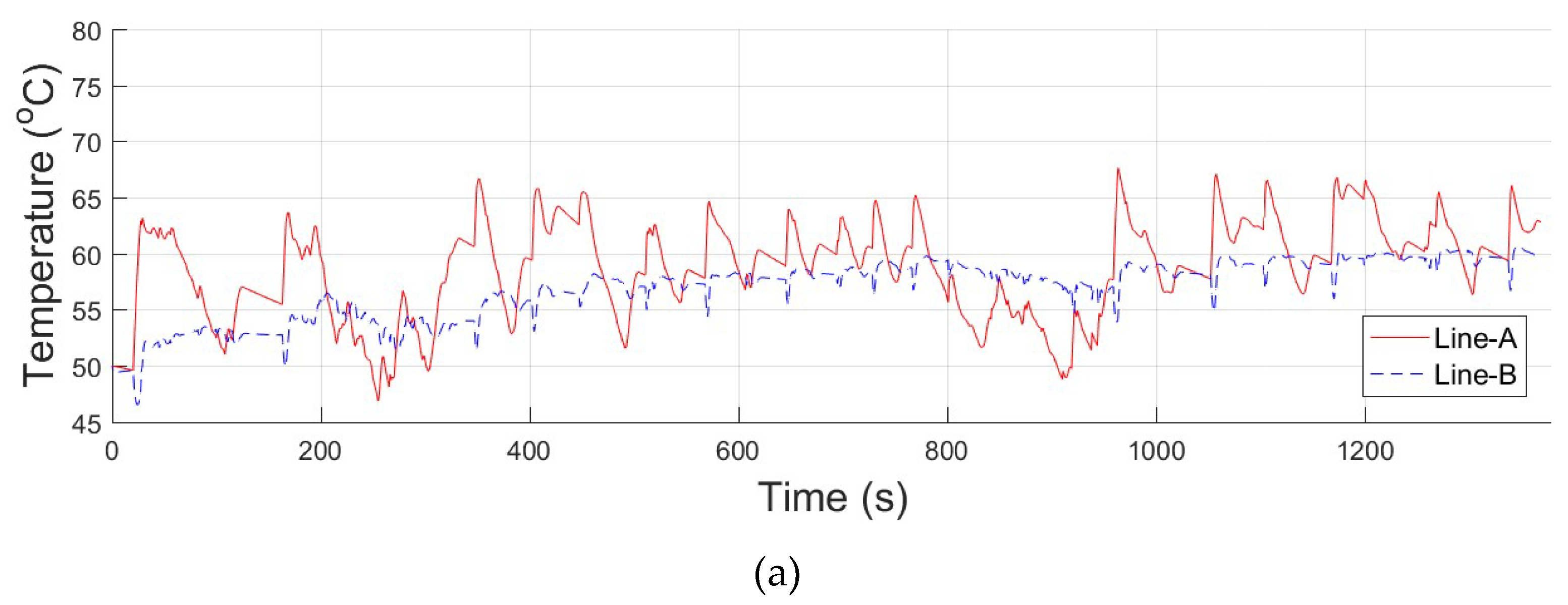
4. Results and Discussion
5. Conclusions
Author Contributions
Funding
Conflicts of Interest
Abbreviations
| FTP | Federal test procedure |
| HHV | Hydraulic hybrid vehicle |
| HP | High pressure |
| HST | Hydrostatic transmission |
| LP | Low pressure |
| UDDS | Urban dynamometer driving schedule |
References
- Baseley, S.; Ehret, C.; Greif, E.; Kliffken, M.G. Hydraulic hybrid systems for commercial vehicles. SAE Tech. Pap. 2007, 1, 4150. [Google Scholar]
- Li, C.-T.; Peng, H. Optimal configuration design for hydraulic split hybrid vehicles. In Proceedings of the 2010 American Control Conference, Baltimore, MD, USA, 30 June–2 July 2010; pp. 5812–5817. [Google Scholar]
- Daher, N.; Ivantysynova, M. Energy analysis of an original steering technology that saves fuel and boosts efficiency. Energy Convers. Manag. 2014, 86, 1059–1068. [Google Scholar] [CrossRef]
- Chen, Q.; Lin, T.; Ren, H.; Fu, S. Novel potential energy regeneration systems for hybrid hydraulic excavators. Math. Comput. Simul. 2019, 163, 130–145. [Google Scholar] [CrossRef]
- Yu, Y.X.; Ahn, K.K. Optimization of energy regeneration of hybrid hydraulic excavator boom system. Energy Convers. Manag. 2019, 183, 26–34. [Google Scholar] [CrossRef]
- Minav, T.; Heikkinen, J.; Schimmel, T.; Pietola, M. Direct driven hydraulic drive: Effect of oil on efficiency in sub-zero conditions. Energies 2019, 12, 219. [Google Scholar] [CrossRef]
- An, K.; Kang, H.; An, Y.; Park, J.; Lee, J. Methodology of excavator system energy flow-down. Energies 2020, 13, 951. [Google Scholar] [CrossRef]
- Bender, F.A.; Bosse, T.; Sawodny, O. An investigation on the fuel savings potential of hybrid hydraulic refuse collection vehicles. Waste Manag. 2014, 34, 1577–1583. [Google Scholar] [CrossRef]
- Heskitt, M.; Smith, T.; Hopkins, J. Design & Development of the LCO-140H Series Hydraulic Hybrid Low Floor Transit Bus; Federal Transit Administration: Washing, DC, USA, 2012.
- Ramdan, M.I.; Stelson, K.A. Optimal design of a power-split hybrid hydraulic bus. Proc. Inst. Mech. Eng. Part D J. Automob. Eng. 2016, 230, 1699–1718. [Google Scholar] [CrossRef]
- Bravo, R.R.S.; De Negri, V.J.; Oliveira, A.A.M. Design and analysis of a parallel hydraulic - pneumatic regenerative braking system for heavy-duty hybrid vehicles. Appl. Energy 2018, 225, 60–77. [Google Scholar] [CrossRef]
- Pugi, L.; Pagliai, M.; Nocentini, A.; Lutzemberger, G.; Pretto, A. Design of a hydraulic servo-actuation fed by a regenerative braking system. Appl. Energy 2017, 187, 96–115. [Google Scholar] [CrossRef]
- Wu, W.; Hu, J.; Jing, C.; Jiang, Z.; Yuan, S. Investigation of energy efficient hydraulic hybrid propulsion system for automobiles. Energy 2014, 73, 497–505. [Google Scholar] [CrossRef]
- Ramakrishnan, R.; Hiremath, S.S.; Singaperumal, M. Design strategy for improving the energy efficiency in series hydraulic/electric synergy system. Energy 2014, 67, 422–434. [Google Scholar] [CrossRef]
- Hui, S.; Lifu, Y.; Junqing, J.; Yanling, L. Control strategy of hydraulic/electric synergy system in heavy hybrid vehicles. Energy Convers. Manag. 2011, 52, 668–674. [Google Scholar] [CrossRef]
- Wang, Z.; Jiao, X.; Pu, Z.; Han, L. Energy recovery and reuse management for fuel-electric-hydraulic hybrid powertrain of a construction vehicle. IFAC-PapersOnLine 2018, 51, 390–393. [Google Scholar] [CrossRef]
- Gong, J.; Zhang, D.; Guo, Y.; Liu, C.; Zhao, Y.; Hu, P.; Quan, W. Power control strategy and performance evaluation of a novel electro-hydraulic energy-saving system. Appl. Energy 2019, 233–234, 724–734. [Google Scholar] [CrossRef]
- Du, Z.; Cheong, K.L.; Li, P.Y.; Chase, T.R. Fuel Economy Comparisons of Series, Parallel and HMT hydraulic hybrid architectures. In Proceedings of the 2013 American Control Conference, Washington, DC, USA, 17–19 June 2013; pp. 5974–5979. [Google Scholar]
- Wang, Y.; Zeng, X.; Song, D.; Yang, N. Optimal rule design methodology for energy management strategy of a power-split hybrid electric bus. Energy 2019, 185, 1086–1099. [Google Scholar] [CrossRef]
- Pei, H.; Hu, X.; Yang, Y.; Tang, X.; Hou, C.; Cao, D. Configuration optimization for improving fuel efficiency of power split hybrid powertrains with a single planetary gear. Appl. Energy 2018, 214, 103–116. [Google Scholar] [CrossRef]
- Sim, T.P.; Li, P.Y. Analysis and control design of a hydro-mechanical hydraulic hybrid passenger vehicle. In Proceedings of the ASME 2009 Dynamic Systems and Control Conference, Hollywood, CA, USA, 12–14 October 2009; pp. 667–674. [Google Scholar]
- Li, P.Y. Optimization and control of a hydro-mechanical transmission based hybrid hydraulic passenger vehicle. In Proceedings of the 7th International Fluid Power Conference, Aachen, Germany, 22–24 March 2010. [Google Scholar]
- Cheong, K.L.; Li, P.Y.; Chase, T.R. Optimal design of power-split transmissions for hydraulic hybrid passenger vehicles. In Proceedings of the 2011 American Control Conference, San Francisco, CA, USA, 29 June–1 July 2011; pp. 3295–3300. [Google Scholar]
- Zhang, H.; Wang, F.; Stelson, K.A. Modeling and design of a hydraulic hybrid powertrain for passenger vehicle. In Proceedings of the ASME/BATH 2017 Symposium on Fluid Power and Motion Control, Sarasota, FL, USA, 16–19 October 2017. [Google Scholar]
- Cheong, K.L.; Du, Z.; Li, P.Y.; Chase, T.R. Hierarchical control strategy for a hybrid hydro-mechanical transmission (HMT) power-train. In Proceedings of the American Control Conference, Portland, OR, USA, 4–6 June 2014; pp. 4599–4604. [Google Scholar]
- Kumar, R.; Ivantysynova, M. An optimal power management strategy for hydraulic hybrid output coupled power-split transmission. In Proceedings of the ASME Dynamic Systems and Control Conference, Hollywood, CA, USA, 12–14 October 2009; pp. 299–306. [Google Scholar]
- Kumar, R.; Ivantysynova, M. The hydraulic hybrid alternative for Toyota Prius—A power management strategy for improved fuel economy. In Proceedings of the 7th International Fluid Power Conference, Aachen, Germany, 22–24 March 2010. [Google Scholar]
- Lammert, M.P.; Burton, J.; Sindler, P.; Duran, A. Hydraulic hybrid and conventional parcel delivery vehicles’ measured laboratory fuel economy on targeted drive cycles. SAE Int. J. Altern. Powertrains 2015, 4, 11–19. [Google Scholar] [CrossRef]
- Wasbari, F.; Bakar, R.A.; Gan, L.M.; Tahir, M.M.; Yusof, A.A. A review of compressed-air hybrid technology in vehicle system. Renew. Sustain. Energy Rev. 2017, 67, 935–953. [Google Scholar] [CrossRef]
- Macor, A.; Benato, A.; Rossetti, A.; Bettio, Z. Study and simulation of a hydraulic hybrid powertrain. Energy Procedia 2017, 126, 1131–1138. [Google Scholar] [CrossRef]
- Kwon, H.; Sprengel, M.; Ivantysynova, M. Thermal modeling of a hydraulic hybrid vehicle transmission based on thermodynamic analysis. Energy 2016, 116, 650–660. [Google Scholar] [CrossRef]
- Panchal, S.; Dincer, I.; Agelin-Chaab, M. Thermodynamic analysis of hydraulic braking energy recovery systems for a vehicle. J. Energy Resour. Technol. 2016, 138, 011601. [Google Scholar] [CrossRef]
- Kwon, H.; Ivantysynova, M. System and thermal modeling for a novel on-road hydraulic hybrid vehicle by comparison with measurements in the vehicle. In Proceedings of the ASME/BATH 2017 Symposium on Fluid Power and Motion Control, Sarasota, FL, USA, 16–19 October 2017. [Google Scholar]
- Kwon, H.; Keller, N.; Ivantysynova, M. Thermal management of open and closed circuit hydraulic hybrids-A comparison study. In Proceedings of the 11th IFK International Conference on Fluid Power, Aachen, Germany, 19–21 March 2018. [Google Scholar]
- Wu, G.; Zhang, X.; Dong, Z. Powertrain architectures of electrified vehicles: Review, classification and comparison. J. Franklin Inst. 2015, 352, 425–448. [Google Scholar] [CrossRef]
- Conlon, B. Comparative analysis of single and combined hybrid electrically variable transmission operating modes. In Proceedings of the SAE 2005 World Congress and Exhibition, Detroit, MI, USA, 11–14 April 2005. [Google Scholar]
- Bhattacharya, T.K.; Chandra, R.; Mishra, T.N. Performance characteristics of a stationary constant speed compression ignition engine on alcohol-diesel microemulsions. Agric. Eng. Int. CIGR Ejournal 2006, 8, 1–18. [Google Scholar]
- Bhavesh, V.; Rathod, G.P.; Patel, T.M. Performance characteristics of constant speed diesel engine by using of HHO gas and varying injection pressure. Indian J. Res. 2016, 5, 91–94. [Google Scholar]
- Ivantysyn, J.; Ivantysynova, M. Hydrostatic Pumps and Motors; Akademia Books International: Delhi, India, 2001. [Google Scholar]
- Shang, L.; Ivantysynova, M. Scaling criteria for axial piston machines based on thermo-elastohydrodynamic effects in the tribological interfaces. Energies 2018, 11, 3210. [Google Scholar] [CrossRef]
- Klop, R.; Ivantysynova, M. Investigation of noise sources on a series hybrid transmission. Int. J. Fluid Power 2011, 12, 17–30. [Google Scholar] [CrossRef]
- Boetcher, S.K.S. Natural Convection from Circular Cylinders; Springer: Berlin, Germany, 2014. [Google Scholar]
- Stephan, P.; Kabelac, S.; Kind, M.; Martin, H.; Mewes, D.; Schaber, K. VDI Heat Atlas; Springer: Berlin, Germany, 2014. [Google Scholar]
- Churchill, S.W.; Chu, H.H.S. Correlating equations for laminar and turbulent free convection from a vertical plate. Int. J. Heat Mass Transf. 1975, 18, 1323–1329. [Google Scholar] [CrossRef]
- Sparrow, E.M.; Stretton, A.J. Natural convection from variously oriented cubes and from other bodies of unity aspect ratio. Int. J. Heat Mass Transf. 1985, 28, 741–752. [Google Scholar] [CrossRef]
- Oppermann, M. A New Approach for Failure Prediction in Mobile Hydraulic Systems; VDI-Verlag: Düsseldorf, Germany, 2007. [Google Scholar]
- Sprengel, M. Influence of Architecture Design on the Performance and Fuel Efficiency of Hydraulic Hybrid Transmissions. Ph.D. Thesis, Purdue University, West Lafayette, IN, USA, 2015. [Google Scholar]
- Incropera, F.P.; DeWitt, D.P. Fundamentals of Heat and Mass Transfer; Wiley: Hoboken, NJ, USA, 2001. [Google Scholar]


| Standing Gear Ratio | 1.8 |
| Displacement Volume of Unit-1 | 45 cc |
| Displacement Volume of Unit-2 | 62 cc |
| HP Accumulator Volume | 31.5 L |
| LP Accumulator Volume | 31.5 L |
| HP Accumulator Precharge Pressure | 90 bar |
| LP Accumulator Precharge Pressure | 16 bar |
| Maximum System Pressure | 420 bar |
| Low-Pressure Setting | 20 bar |
| Mode | Engine | Unit-1 | Accumulator | Unit-2 | Driveline | Note |
|---|---|---|---|---|---|---|
| 1 | Idle | Idle | Idle | Idle | Idle | - |
| 2 | Motoring | Pumping | Charging | Motoring | Driving | Power Additive |
| 3 | Motoring | Pumping | Idle | Motoring | Driving | |
| 4 | Motoring | Pumping | Discharging | Motoring | Driving | |
| 5 | Motoring | Idle | Idle | Idle | Driving | Full Mechanical |
| 6 | Motoring | Motoring | Charging | Pumping | Driving | Power Recirculation |
| 7 | Motoring | Motoring | Idle | Pumping | Driving | |
| 8 | Motoring | Motoring | Discharging | Pumping | Driving | |
| 9 | Idle | Idle | Charging | Pumping | Braking | - |
| Mode | Engine | Unit-1 | Unit-2 | Driveline | Note |
|---|---|---|---|---|---|
| 1 | Idle | Idle | Idle | Idle | - |
| 2 | Motoring | Pumping | Motoring | Driving | Power Additive |
| 3 | Motoring | Idle | Idle | Driving | Full Mechanical |
| 4 | Motoring | Motoring | Pumping | Driving | Power Recirculation |
| 5 | Idle | Idle | Pumping | Braking | - |
| Forced Convection | Laminar flow: () Turbulent flow: () |
| Free Convection | Cylinder shape: Cube shape: |
© 2020 by the authors. Licensee MDPI, Basel, Switzerland. This article is an open access article distributed under the terms and conditions of the Creative Commons Attribution (CC BY) license (http://creativecommons.org/licenses/by/4.0/).
Share and Cite
Kwon, H.; Ivantysynova, M. System Characteristics Analysis for Energy Management of Power-Split Hydraulic Hybrids. Energies 2020, 13, 1837. https://doi.org/10.3390/en13071837
Kwon H, Ivantysynova M. System Characteristics Analysis for Energy Management of Power-Split Hydraulic Hybrids. Energies. 2020; 13(7):1837. https://doi.org/10.3390/en13071837
Chicago/Turabian StyleKwon, Hyukjoon, and Monika Ivantysynova. 2020. "System Characteristics Analysis for Energy Management of Power-Split Hydraulic Hybrids" Energies 13, no. 7: 1837. https://doi.org/10.3390/en13071837
APA StyleKwon, H., & Ivantysynova, M. (2020). System Characteristics Analysis for Energy Management of Power-Split Hydraulic Hybrids. Energies, 13(7), 1837. https://doi.org/10.3390/en13071837