Article

An Energy Graph-Based Approach to Fault Diagnosis of a Transcritical CO2 Heat Pump

by
Kenneth R. Uren
1,*,
George van Schoor
2,
Martin van Eldik
3 and
Johannes J. A. de Bruin
1
1
School of Electrical, Electronic and Computer Engineering, North-West University, Potchefstroom 2520, South Africa
2
Unit for Energy and Technology Systems, Faculty of Engineering, Potchefstroom 2520, South Africa
3
School of Mechanical Engineering, North-West University, Potchefstroom 2520, South Africa
*
Author to whom correspondence should be addressed.
Energies 2020, 13(7), 1783; https://doi.org/10.3390/en13071783
Submission received: 14 February 2020 / Revised: 19 March 2020 / Accepted: 30 March 2020 / Published: 7 April 2020

Abstract

:
The objective of this paper is to describe an energy-based approach to visualize, identify, and monitor faults that may occur in a water-to-water transcritical CO 2 heat pump system. A representation using energy attributes allows the abstraction of all physical phenomena present during operation into a compact and easily interpretable form. The use of a linear graph representation, with heat pump components represented as nodes and energy interactions as links, is investigated. Node signature matrices are used to present the energy information in a compact mathematical form. The resulting node signature matrix is referred to as an attributed graph and is populated in such a way as to retain the structural information, i.e., where the attribute points to in the physical system. To generate the energy and exergy information for the compilation of the attributed graphs, a descriptive thermal–fluid model of the heat pump system is developed. The thermal–fluid model is based on the specifications of and validated to the actual behavioral characteristics of a physical transcritical CO 2 heat pump test facility. As a first step to graph-matching, cost matrices are generated to represent a characteristic residual between a normal system node signature matrix and a faulty system node signature matrix. The variation in the eigenvalues and eigenvectors of the characteristic cost matrices from normal conditions to a fault condition was used for fault characterization. Three faults, namely refrigerant leakage, compressor failure and gas cooler fouling, were considered. The paper only aims to introduce an approach, with the scope limited to illustration at one operating point and considers only three relatively large faults. The results of the proposed method show promise and warrant further work to evaluate its sensitivity and robustness for small faults.

1. Introduction

A heat pump system extracts heat from natural sources such as air, surface water or solar energy and use it in a thermodynamic cycle. Heat pump technology is widely used in many applications that warrant cooling, heating or both. What distinguishes the considered CO 2 heat pump in this paper from chillers and other heat pumps is the fact that it is a water-to-water system and produces both hot and cold water as useful products.
According to Zogg [1], when considering the ecological and economic impact of refrigerating machines, air-conditioners, and heat pumps, the main issue is to maximize the efficiency to minimize energy consumption. This is motivated due to the global drive towards mitigating CO 2 emissions. Zogg also refers to a field survey [2] that indicates that the average energetic efficiencies of the heat pumps installed in Swiss buildings were about 10% lower than the efficiencies measured under standard laboratory conditions. It was also found that for some installations the performance degradation was as high as 30%. A similar study in the United States of over 55,000 air conditioning units showed that more than 90% were operating with one or more kinds of faults [3]. Yet another study surveying roof-top units indicates an operating efficiency of 80% of designed performance with 63% of these units having performance degradation due to refrigerant leakage [4]. These observations motivate the need for diagnostic techniques which ideally can monitor these energy conversion systems during transient and steady-state operating conditions.
In the review papers by Zhao et al., and Shi and O’Brien [5,6] the classification of fault detection methods for energy systems are presented. Fault detection methods can be classified into two subcategories: data-based and knowledge-based. The knowledge-based methods rely on domain and prior knowledge to derive rules or models which generally have clear physical meaning. Data-based methods in contrast detect faults through finding the changes of patterns in process measurements. Patterns extracted from industrial systems by means of data-driven algorithms do not usually have physical meaning. According to Zhao et al., knowledge-based methods have been dominant from the 1980s till around 2005 and since then the data-based methods became more prominent. Shi and O’Brien also confirm that since 2010 research on building fault detection and diagnosis (FDD) systems has steadily increased with a specific focus on black-box modeling.
The most widely used data-driven FDD technique for heat pump systems is principal component analysis (PCA), which is a multivariate statistical analysis approach [7,8]. This approach allows transformation of several related variables to a smaller set of uncorrelated variables. It is ideal for feature extraction as well as sensor validation and reconstruction. Chen et al. [9] applied this approach successfully on an air-source heat pump. Another successful technique often implemented is artificial neural network modeling due to its ability to predict complex system features [10].
Despite the success of data-driven methods, future fault diagnosis methods will need to meet a variety of system needs and challenges such as robustness, uncertainty handling, and big data processing. According to Severson et al. [11] this will call for new methods to draw from the strengths of both knowledge- and data-based approaches to form what is called hybrid techniques [12].
The energy-based visualization concept was first introduced by van Schoor et al. [13]. This concept aims to address condition monitoring, control and optimization of large-scale industrial plants in a generic way using energy as the main parameter. Marais et al. [14] evaluated the concept on a continuous stirred tank reactor (CSTR) using heat flow rate for condition monitoring. Another application of energy-based condition monitoring at component level was illustrated by Uren et al. [15] where power and energy parameters were used for deriving energy signatures characterizing a counter-flow heat exchanger. The energy signatures were used to derive graphical energy residuals for fault detection. The energy concept was then evaluated using an energy threshold method applied to an autothermal reformer [16]. The importance of capturing structural information for fault isolation purposes was realized. Therefore, attributed graph representations were introduced by [17] to combine energy and structural information in a holistic way. This energy graph-based approach was improved by extracting eigenvector information from a graph cost matrix [18]. The aim with of using eigenvector information is to obtain more descriptive residuals for fault detection and diagnosis. In thermal–fluid and chemical processes it became evident that more descriptive parameters such as entropy and exergy should be used for condition monitoring [19,20]. These parameters also characterize irreversibilities in the process. Greyling et al. [21] illustrates an exergy-based fault detection method on a gas-to-liquids (GTL) process, illustrating the usability of the energy approach to FDD on a system level.
This paper extends the work presented on the energy graph-based method and contributes a fault detection and identification methodology that combines a data-driven pattern recognition technique called graph-matching, and system knowledge in terms of exergy and energy flow. This methodology is evaluated on a validated heat pump system model.
This paper is outlined as follows: Section 2 discusses the heat pump test facility used to obtain practical system data. In Section 3 a system-level model of the heat pump system is derived and discussed. The model is simulated in the EES ® environment and validated with practical data. Section 4 introduces the energy graph-based characterization approach using energy and exergy information and then Section 5 follows with the energy graph-based fault detection and isolation methodology. The results are discussed in Section 6 followed by conclusions in Section 7.

2. System Description

Figure 1 illustrates the water-to-water transcritical CO 2 (R744) heat pump system with its main cyclic points and components shown. The typical thermodynamic behavior of the transcritical refrigerant loop is shown in Figure 2 on a T-s diagram.
The transcritical R744 cycle extracts heat from the water stream that flows through the evaporator component. The R744 that flows through the evaporator is therefore heated and the corresponding water stream is cooled. The R744 that enters the evaporator from the expansion valve (EV) is in a two-phase state. The R744 is heated in the evaporator until it reaches a saturated vapor state—cycle point (1). Thereafter it is heated further until it reaches a superheated vapor state—cycle point (2). Superheating is performed to increase the efficiency of the transcritical cycle and to avoid compressing a two-phase stream. Compression of a two-phase mixture that contains liquid droplets will result in compressor damage. The compressor component receives the superheated gas that leaves the evaporator and compresses the gas to a higher pressure and temperature condition as indicated in Figure 2 between cycle point (2) and (3). The R744 that is discharged from the compressor is in the supercritical gaseous state. The gas cooler component receives the high-temperature supercritical gas and transfers heat from the supercritical gas to the water stream. The R744 that flows through the gas cooler is cooled and the corresponding water stream is heated. In a transcritical heat pump, the heat exchanger component that rejects heat from the refrigerant is called a gas cooler since the R744 that flows through it remains in a supercritical state during the heat rejection process. The process of condensation, as found in a typical Freon heat pump cycle, does not take place.
The R744 in the gas cooler component may be in either the supercritical gaseous or in the sub-cooled liquid state—cycle point (23). For proper system operation, the EV should receive R744 that is in the sub-cooled liquid state. Within the expansion valve, R744 undergoes an isenthalpic throttling process—cycle point (23) to (24). The throttling process causes the R744 to undergo a significant pressure drop. The temperature of the R744 also decreases with the reduction in its pressure. The throttling process effectively lowers the temperature so that evaporation of the R744 may again take place, via heat transfer from the water stream to the R744 in the evaporator component—cycle point (24) to (2). The actual heat pump test facility viewed from the front and the back is illustrated in Figure 3. Table 1 lists the corresponding components found in the heat pump system with their respective functions.

3. System Model

The system model is developed in the Engineering Equation Solver (EES ® ) environment [23]. The simulation methodology follows a systems-level approach. Semi-theoretical models are used during the implementation of conservation laws to solve for the required parameters which quantify the behavioral properties of the components in the system. The laws of conservation of mass, momentum and energy (for steady incompressible flow) are each applied to every component in the system. The use of the incompressible form of the conservation of momentum law is valid due to the Mach number of the refrigerant never exceeding 0.1 throughout the system within the range of simulated system conditions. At flow Mach numbers below 0.3, the compressible and incompressible form of the law of conservation of momentum both yield the same thermo-physical property results. The law of conservation of mass for steady incompressible flow through an individual component’s control volume (CV) is expressed as [24]:
i = 1 n 1 m ˙ i n | i = j = 1 n 2 m ˙ o u t | j ,
where the first term is the summation of all the mass flow streams entering the CV and the second term is the summation of all the mass flow streams flowing out of the CV. The conservation of mass for every system component may thus be simplified to:
m ˙ i n = m ˙ o u t .
The law of conservation of momentum for steady (incompressible low Mach number) flow through an individual component’s CV is expressed as [24]:
i = 1 n 1 ( P t o t ) i n | i + j = 1 n 2 ( ρ g z ) i n | j = k = 1 n 3 ( P t o t ) o u t | k + l = 1 n 4 ( ρ g z ) o u t | l + Δ P t o t ,
where the first and second terms are the total and hydrostatic pressures of fluids entering the CV, the third and fourth terms are the total- and hydrostatic pressures of fluids leaving the CV and the fifth term is the pressure drop which occurs as the various interacting fluids flow through the CV. Equation (3) may be simplified by only considering the interacting fluids for each component. The conservation of momentum for the refrigerant side of the evaporator, gas cooler, EV and compressor components is given by:
( P t o t | g ) i n = ( P t o t | g ) o u t + Δ P t o t | g ,
where the subscript, g, refers to the R744 refrigerant. The conservation of momentum for the water side of the evaporator and gas cooler components is given by:
( P t o t | w ) i n = ( P t o t | w ) o u t + Δ P t o t | w ,
where the subscript, w, refers to the water stream. The pressure ratio of the compressor is used to find the discharge pressure of the refrigerant leaving the compressor. The pressure ratio for a compressor is defined as [22]:
r P = P t o t | g , o u t l e t P t o t | g , i n l e t .
Finally, the law of conservation of energy (First Law of Thermodynamics) for a steady flow process of an individual component’s CV is given by [24]:
Q ˙ n e t + W ˙ n e t + i = 1 n 1 ( m ˙ h t o t ) i n | i + j = 1 n 2 ( m ˙ g z ) i n | j = k = 1 n 3 ( m ˙ h t o t ) o u t | k + l = 1 n 4 ( m ˙ g z ) o u t | l ,
where the first term is the net heat transfer into the CV, the second term is the net work absorbed by the CV, the third term is the total flow energy entering the CV, the fourth term is the gravitational potential energy of the flow(s) entering the system, the fifth term represents the flow energy leaving the CV, and the sixth term represents the gravitational potential energy of the flow(s) departing the CV. The conservation of energy for each component was compiled under the assumption that the elevation head difference throughout the system is negligible. The elevation head difference for the experimental system is 0.5 m. The conservation of energy for the evaporator and gas cooler component is given by:
( m ˙ g h t o t | g ) i n + ( m ˙ w h t o t | w ) i n = ( m ˙ g h t o t | g ) o u t + ( m ˙ w h t o t | w ) o u t .
The conservation of energy for the compressor component is given by:
( m ˙ g h t o t | g ) i n + W ˙ C = ( m ˙ g h t o t | g ) o u t .
The expansion valve component’s throttling process is assumed to be isenthalpic. Under the isenthalpic assumption, the conservation of energy for the expansion valve simplifies to:
( m ˙ g h t o t | g ) i n = ( m ˙ g h t o t | g ) o u t .
In addition to the traditional conservation laws, an exergy balance was also applied to solve for its corresponding internal irreversibility rate within each system component. An exergy balance for an individual component’s CV has the form [25]:
E ˙ C V Q + W ˙ n e t + i = 1 n 1 ( E ˙ ) i n | i = j = 1 n 2 ( E ˙ ) o u t | j + I ˙ R ,
where the first term is the exergy transfer to the CV due to heat transfer, the second term is the net work absorbed by the CV, the third term is the exergy entering the CV, the fourth term is exergy leaving the CV and the fifth term is the rate at which exergy is irreversibly destroyed inside of the CV. The evaporator and gas cooler components do not have associated work terms in their respective exergy balance equations. The exergy balance for the evaporator is given by:
E ˙ g i n + E ˙ w i n = E ˙ g o u t + E ˙ w o u t + I ˙ E .
The work term is omitted in (11) and (12) since no work is done on the working fluid in these components, only heat transfer takes place. The exergy balance for the gas cooler component is identical to the exergy balance for the evaporator component, as in (12), with the only difference being that the irreversibility rate’s subscript changes to GC. The exergy balance for the compressor component is given by:
E ˙ g i n + W ˙ C = E ˙ g o u t + I ˙ C .
The exergy balance for the expansion valve component is given by:
E ˙ g i n = E ˙ g o u t + I ˙ E V .
To validate the EES ® system model, experimental results for expansion valve (EV) openings of 30%, 40%, 50%, 60% and 70% were compared to the simulation results for the same operating conditions. The results for an EV orifice opening of 30% are discussed in detail whereafter the results for the other conditions are merely summarized. The system input parameters for the 30% EV orifice opening condition are summarized in Table 2.
Figure 4 shows the experimental and simulation results overlaid on a T-s diagram. The pressures are also indicated on the figure for the gas side. The pressure on the water side is in the order of 200 kPa. Similarly, Figure 5 shows the overlaid results and simulation results on a log. P-h diagram.
Table 3 shows the key parameter values associated with the 30% EV orifice opening operating point illustrated in Figure 4 and Figure 5 with the deviation between the simulated and test bench parameter values for the operating point.
Table 3 reveals satisfactory validation of the EES ® system model for the 30% EV orifice opening condition. When considering EV orifice opening results for 40%, 50%, 60% and 70% together with the 30% case, the patterns produced when plotting successive property diagrams for the simulated and measured cases, were similar. As the EV orifice opening is increased, the area encapsulated by the refrigerant cycle property plot decreases in overall size. As the EV orifice opening is increased the percentage deviation between the simulated and test bench results gradually increases as summarized in Table 4. At 60% EV orifice opening the deviation becomes unacceptably high. The reason for the higher deviations at larger EV orifice openings is two-fold; less data was available at these operating points together with the fact that the cycle is not fully developed or thermodynamically stable at the larger EV orifice openings. The EES ® system model shows satisfactory prediction (if the maximum deviation of 10.7% is viewed as acceptable) of the heat pump’s energy characteristics for the 30%, 40% and 50% EV orifice opening operating points under the condition that the enthalpy associated with the expansion valve’s throttling process is at a value smaller than the critical enthalpy of the system’s refrigerant. The 30% working point is however used for the analysis results as this represents an operating point where the cycle is fully developed and where the simulation accurately represents the test bench.
The modeling of the heat pump system should incorporate the interdependent behavior that is a characteristic of the series connected system components. The modeling and characterization of each component in the system and that of the transcritical cycle will be fundamentally based on the control volume approach of thermal–fluid analysis.
The conservation equations and exergy balance equations for system components will be derived under the assumption that the heat pump system and all its components are operating under steady-state conditions. In the range of heat pump operating conditions investigated in this study the flow regime of the refrigerant and the two interacting water streams is always turbulent. The Nusselt number correlations that are used in the simulation to predict convection coefficient values are thus for turbulent flow. The finite term and incompressible flow form of the conservation of momentum equation will be used for the modeling of the heat pump system components. This assumption is valid even for the compressible carbon dioxide refrigerant due to the low Mach number values associated with the carbon dioxide flow. The effect of elevation height difference between system components is assumed to be negligible in the compilation of the conservation of momentum equations for the system’s components.
To ensure component interdependency, it will be assumed in the composition of the conservation and component-specific equations that the input values of the devised control volume regions are known. The output thermo-physical properties of the associated CV regions will then be predicted by solving the parameters associated with the conservation and component-specific equations. The component interactions and interdependency will be interlaced in the EES ® environment by setting the output of each component equal to the input of the component that chronologically succeeds it in the transcritical cycle. Implementation of this approach assures that the operational characteristics of each component in the system are directly dependent on the output of the component that precedes it. Detail on the model derivation can be found in Appendix A.

4. Energy Graph-Based Characterization

Graphs can be used to represent interactions of large-scale and complex systems in a structured way [26]. Some useful and descriptive attributes can be assigned to a graph which may then be called an attributed graph [27]. This type of graph also allows structural information and attributes to be associated with specific locations in the actual system being considered [28]. This structural property may contribute significantly in terms of fault isolation. Different approaches can be followed when using energy-based attributes. First, the choice of what constitutes a link and what constitutes a node needs to be determined. In this case, a node is defined as a system component e.g., a compressor or turbine, and a link is defined as a connection between two system components. In the following sections this approach will be discussed in more detail from a graph-theoretic point of view and how it relates to the heat pump system considered.

4.1. Graph-Theoretic Concepts

According to Rahman [29], a graph G can be defined as a tuple ( V , E ) consisting of a finite set V of vertices and a finite set E of edges. Each edge can be represented by an unordered pair of vertices. For example, and edge e between two vertices u and v may be represented as ( u , v ) . Balakrishnan and Ranganathan [30] gives the following formal mathematical definition of a graph: “A graph is an ordered triple G = ( V ( G ) , E ( G ) , I G ) , where V ( G ) is a nonempty set, E ( G ) is set disjoint from V ( G ) , and I G is an “incidence” relation that associates with each element of E ( G ) an unordered pair of elements (same or distinct) of V ( G ) .” The symbol G is thus used to denote the graph as a whole, V ( G ) represents the vertices of the said graph, E ( G ) is the graph edges and I G is the connection relation between the vertices and edges of the graph. Figure 6 illustrates an example of a linear graph.
In the context of graph theory terminology, the term vertices may be used interchangeably with the term nodes, and the term edges may be used interchangeably with the term links. The author will henceforth refer to nodes and links.

4.2. Heat Pump System Graph Representation

An attributed graph is a graph representation that is assigned a set of parameters with numerical values [17]. An attributed graph is useful for system representation since numerous graph-matching operations may be performed on the node signature matrices that are compiled from attributed graphs [29]. A node signature matrix is merely a representation of an attributed graph’s attributed parameters in matrix format [31]. The investigated heat pump system has four components. Nodes will be used to represent the four components and links will be used to represent the energy that flows in and out of the components. The approach followed in this paper is similar to the approach outlined in van Schoor & Uren [19], the only difference being that in this work the heat exchanger is assigned a single node with four energy links.
The attributed graph representation of the heat pump system is illustrated in Figure 7. The nodes are indicated with symbol n and the links are indicated with symbol l. The node with the number zero as a subscript is defined as the reference node. The inclusion of a zero node enables the structuring of the graph with its attributes while maintaining the structural information of the graph [19]. Following the approach of van Schoor & Uren [19] the general node signature matrix for the graph in Figure 7 is obtained as:
M ag = n 0 l 00 l 01 l 02 l 03 l 04 n 1 l 10 l 11 l 12 l 13 l 14 n 2 l 20 l 21 l 22 l 23 l 24 n 3 l 30 l 31 l 32 l 33 l 34 n 4 l 40 l 41 l 42 l 43 l 44 .
M ag is structured with the first column allocated for the node attributes and the subsequent columns for the link attributes. For the link attributes the first numeral in the subscript refers to the origin of the link and the second refers to the destination. A subscript, “01”, indicates that the link is directed from node number zero to node number one. The links in the proposed graph representation thus encode information on the magnitude and the direction of the attributed parameters. In this manner, each row of the matrix represents attributes associated with a specific node.
The links that do not appear in Figure 7 are assigned values of zero. Equation (15) may thus be simplified by populating the entries of the matrix with zeros for the positions that represent links that are not present in the graph representation. A link attribute will also be assigned if its subscript notation is opposite to the flow direction assigned. The rule of l m n = l n m will therefore be used to determine whether to assign a link attribute a positive or negative sign. In this way, the structural information of the linear graph is encoded during matrix compilation. The reduced attributed graph node signature matrix that results for the heat pump system after eliminating redundant links, is given by:
M rag = n 0 0 l 01 l 02 l 03 0 n 1 l 10 0 l 12 0 l 41 n 2 l 02 l 12 0 l 23 0 n 3 l 30 0 l 23 0 l 34 n 4 0 l 41 0 l 34 0 .
The graph representation of the heat pump will use the rates of exergy destruction of the associated components as the node attributes. The link attributes will be the energy flow rates in or out of the associated component to which the links are connected. Table 5 lists the attributes that will be assigned to the graph representation of the heat pump.
From inspection of Table 5, it is evident that every parameter assigned to the graph representation is a variable with the same unit, i.e., kilowatt. The assignment of parameters with the same unit to the node signature matrices ensures that the subsequent calculations are performed with variables that represent the same physical property. The heat pump graph representation with the EES ® simulation output parameters assigned as attributes is illustrated in Figure 8.
The reduced attributed graph node signature matrix that results from Figure 8 is given by:
M rag = 0 0 E ˙ w i | E W ˙ C E ˙ w i | G C 0 I ˙ E E ˙ w o | E 0 E ˙ 2 0 E ˙ 24 I ˙ C W ˙ C E ˙ 2 0 E ˙ 3 0 I ˙ G C E ˙ w o | G C 0 E ˙ 3 0 E ˙ 23 I ˙ E E V 0 E ˙ 24 0 E ˙ 23 0 .
With the reduced attributed graph node signature matrix defined, the next step is to illustrate how this system description can be used for fault detection and isolation.

5. Energy Graph-Based Fault Detection and Isolation Method

This section introduces the graph-based concepts of graph-matching and furthermore the idea of eigendecomposition as a means to use the attributed graph node signature matrix for fault detection and isolation.

5.1. Graph-Matching

Graph-matching refers to the methodologies and the algorithms that compare two or more graphs numerically to determine the degree of similarity between their attributes [17]. In the context of fault detection and diagnosis, a fault signature may be defined as a distinct set of attributes that are expressed on a numerical basis for a fault scenario that uniquely identifies a specific operating condition under which a system is operational [32]. Graph-matching will be used in this work to aid in the compilation of fault signatures for different fault scenario. The approach outlined by Jouili & Tabbone [33] will be implemented to perform the matching of two different graphs.
De la Fuente [31] defines a normal condition as: “A system operating under a condition where none of its defining characteristic properties or associated parameters deviates from the standard system condition.” In the context of graphs, the healthy system graph will represent a normal graph with its corresponding normal node signature matrix. Furthermore, de la Fuente [31] defines a fault condition as: “A system operating under a condition where an unpermitted deviation of at least one characteristic property or parameter of the system from the standard condition is present.” In the context of graphs, the faulty system graph will represent a graph characteristic of a specific fault with its corresponding fault node signature matrix.
It is desirable to keep a heat pump system running at its normal condition for the longest period possible during operation. Operating at the normal “healthy” system condition ensures efficient and reliable energy conversion and lowers the overall maintenance required to run the system. A fault scenario for a heat pump system is thus likely to impact the efficiency and economics of the system. This section investigates refrigerant leakage, compressor failure and gas cooler fouling.

5.2. Cost Matrix Generation

A cost matrix, denoted by C , is a matrix that describes the matching costs between two node signature matrices [33]. The method proposed by Jouili & Tabbone [33] may be used to match the same node signature matrix to itself or a node signature matrix with a different set of element values. The matching of an initial node signature matrix that contains parameter values relating to a healthy operating condition, to itself is performed to generate the reference condition to which other operating conditions may be compared. The element entries of a cost matrix thus encode information on the similarity between two compared node signature matrices.
In the method by Jouili & Tabbone [33], the entries of a cost matrix are calculated using a version of the Heterogeneous Euclidean Overlap Method (HEOM). The entries of a cost matrix C are calculated using the HEOM such that [34]:
C i , j = H E O M i , j = a = 1 # c o l δ M R i a , M F j a 2 ,
where i denotes a row entry in the generated cost matrix, and j denotes a column entry in the generated cost matrix. The first entry of a cost matrix, for example, is thus calculated by substituting i and j with 1 such that:
C 1 , 1 = H E O M 1 , 1 = a = 1 # c o l δ M R 1 a , M F 1 a 2 .
The complete cost matrix is compiled from the individual entries as follows:
C = C ( 1 , 1 ) C ( 1 , 2 ) C ( 2 , 1 ) .
The variable a is the number of the column in the applicable node signature matrix. The delta function, δ ( · ) is defined as:
δ M R i a , M F j a = M R i a M F j a r a n g e a , i f r a n g e a 0 M R i a M F j a , i f r a n g e a = 0 ,
where M R i a refers to the i-th row of the reference node signature matrix and M F j a refers to the j-th row of the node signature matrix that is compared to the reference node signature matrix. The range is given by:
r a n g e a = m a x a m i n a ,
where m a x a is the largest numerical entry of the a-th column of the reference node signature matrix and m i n a is the smallest numerical entry in the same column.

5.3. Eigenvectors and Eigenvalues

Lay et al. [35] give a good definition of eigenvalues and eigenvectors. Eigenvectors define a set of properties of those numerical values subject to a linear transformation in n-dimensional space that remain unchanged. The eigenvectors of a linear transformation are those vectors that remain on their spanning line through the origin of the n-dimensional space after a linear transformation [35]. Each eigenvector has associated with it an eigenvalue that encodes information on the change in direction and scaling that the eigenvectors undergo during a linear transformation. The eigenvectors associated with a linear transformation may thus change direction on their linear span and increase or decrease in magnitude, but they always start at the origin of the n-dimensional space and point in a direction along the length of their span.
Eigenvectors and their associated eigenvalues are thus excellent properties that may be used to uniquely characterize, summarize, and represent the data encoded in a matrix [19]. This is the motivation for calculation of the eigenvectors and eigenvalues of the cost matrices.

6. Results and Discussion

This section investigates the use of eigenvectors and eigenvalues of the cost matrices generated by the method by Jouili and Tabbone [33] as a means to fault diagnosis on the heat pump system.

6.1. Analysis Assumptions

Since the paper only aims to introduce the energy graph-based approach to fault diagnosis, the scope of analysis is limited to one operating point and considering only 3 large fault conditions. The analysis assumptions are summarized as follows:

6.1.1. Operating Point

For the results reported in the paper the case of 30% EV orifice opening is taken as the normal conditions operating point with the system input parameters and key cycle parameters as summarized in Table 2 and Table 3 respectively. A smaller orifice opening degree works well since then the thermal-fluid behaviour of the cycle is fully developed.

6.1.2. Fault Conditions

Three fault conditions will be investigated: working fluid leakage from the heat pump, compressor failure, and fouling inside of the gas cooler on the water side. These fault conditions are seen as the main fault categories in heat pumps [36,37].

6.1.3. Variation in Data

Due to parameter variation and measurement uncertainty, a variation in energy and exergy characteristics can be expected which should be seen as part of normal behavior. For the actual test bench, the measurement uncertainty was less than 1% when calculating the heat transfer on the CO 2 side [38]. In this study, variation in data is not included per se. However, a threshold for FDI representative of typical heat pump energy performance variation is chosen. From [39] the typical COP variation that can be expected is in the region of 4%. The threshold for FDI for this study is therefore set at 5%.

6.2. The Normal Case Analyzed

The node signature matrix for the chosen normal case is numerically given by:
M normal = 0 0 44.229 10.834 29.840 0 2.753 19.174 0 9.864 0 34.914 3.088 10.834 9.864 0 0.971 0 1.463 65.725 0 0.971 0 34.914 2.033 0 34.914 0 34.914 0 .
The M normal matrix will thus represent the healthy fault-free case when progressive fault conditions are considered. The normal conditions cost matrix obtained by matching the matrix in (23) to itself is given by:
C normal = 0 1.413 1.750 1.759 1.518 1.413 0 1.071 1.545 1.331 1.750 1.071 0 1.252 1.063 1.759 1.545 1.252 0 1.317 1.518 1.331 1.063 1.317 0 .
The corresponding eigenvalues and eigenvectors of C normal is given by (25) and (26) respectively.
λ 1 5 , n o r m a l = 1.967 , 1.536 , 1.253 , 0.883 , + 5.640 .
v 1 5 , normal = 0.797 + 0.221 + 0.050 0.259 + 0.496 0.089 0.616 0.433 + 0.490 + 0.430 + 0.399 0.360 + 0.017 0.732 + 0.418 + 0.400 + 0.665 0.401 + 0.147 + 0.464 + 0.192 0.005 + 0.806 + 0.368 + 0.422 .
Please note that the eigenvalues and eigenvector components are real numbers. It is also interesting to note that C normal shows symmetry about its main diagonal and that all the entries on the main diagonal are zeros.

6.3. Fault Cases

This section illustrates the implementation of graph-matching to obtain characteristic eigenvalues and eigenvectors for the fault cases of: (1) working fluid leakage, (2) compressor failure and, (3) fouling in the gas cooler.

6.3.1. Working Fluid Leakage

Refrigerant leakage may occur in a system during operations due to material imperfections or vibrations, which will result in a reduction of performance and therefore critical to detect at an early stage. Working fluid leakage was simulated by gradually decreasing the R744 flow rate as input parameter. The flow rate decreased from the normal case of 0.1559 kg/s to 0.0959 kg/s in increments of 0.02 kg/s. The reduced amount of refrigerant flowing through the GC and evaporator causes a reduction in the GC pressure and evaporating pressure. This is expected since at any given time during system operation there is less refrigerant charge inventory inside the heat exchanger components. Since the evaporator and compressor are being starved of refrigerant, the gas cooler will experience the knock-on effect. Starving the gas cooler will reduce the heat load because of limited refrigerant to reject any heat. With less heat to accept (reject from the compressor) the gas cooler will be operating at a lower temperature and pressure. The simulation results correspond to the results found in the study by Zhang & Dong et al. [40] who also found that gas cooler and evaporator pressure decreases with a decrease in total refrigerant mass flow rate in their investigated system. For the normal case the mass flow rate was programmed as a function of the EV orifice opening (refer to (A52) in Appendix A).
The node signature matrix obtained for the fluid leakage fault condition ( m ˙ R 744 = 0.0959 kg/s) is numerically given by:
M F , leak = 0 0 44.229 8.833 29.840 0 2.962 28.028 0 5.848 0 22.048 2.462 8.833 5.848 0 2.985 0 1.250 54.874 0 2.985 0 22.048 1.702 0 22.048 0 22.048 0 .
The leakage fault condition cost matrix obtained by matching M normal to M F , leak is given by:
C leak = 0.170 1.488 1.588 1.740 1.399 1.413 0.409 1.051 1.518 1.187 1.667 0.799 0.220 1.135 0.834 1.668 1.215 1.150 0.296 1.132 1.422 1.130 0.971 1.204 0.328 .
The corresponding eigenvalues and eigenvectors of C leak are given by (29) and (30) respectively:
λ 1 5 , l e a k = + 5.467 , 1.683 , 0.520 , 1.072 , 0.769 .
v 1 5 , leak = + 0.506 + 0.812 + 0.096 0.011 0.038 + 0.457 + 0.016 0.448 0.568 0.608 + 0.394 0.441 + 0.772 0.328 + 0.073 + 0.450 0.344 0.004 + 0.753 0.149 + 0.421 0.165 0.441 + 0.051 + 0.776 .

6.3.2. Compressor Failure

Compressor failure may occur when the seal and mechanisms inside a compressor wear with use [36]. Compressor failure was simulated by assigning a fixed value for isentropic efficiency and gradually decreasing it as input parameter from 0.6527 to 0.5027 in increments of 0.05. For the normal case the isentropic efficiency was however determined as a function of the compressor pressure ratio (refer to (A30) in Appendix A). The node signature matrix obtained for the compressor failure fault condition (isentropic efficiency = 0.5027) is numerically given by:
M F , fail = 0 0 44.229 11.391 29.840 0 1.816 17.570 0 10.504 0 37.126 4.643 11.391 10.504 0 0.887 0 1.715 67.853 0 0.887 0 37.126 1.460 0 37.126 0 37.126 0 .
Please note that the rate of irreversibility generated in the compressor (indicated in red) is high relative to the other irreversibility parameter values in the first column of the matrix (31). The effect of compressor failure on the heat pump’s thermo-physical behavior is thus reflected directly in the increased magnitude of exergy destruction that takes place inside of the compressor. The compressor failure fault condition cost matrix obtained by matching M normal to M F , fail is given by:
C fail = 0.047 1.250 2.085 1.801 1.467 1.416 0.311 1.233 1.553 1.409 1.775 1.190 0.504 1.255 1.183 1.786 1.555 1.539 0.092 1.339 1.547 1.356 1.322 1.339 0.193 .
The corresponding eigenvalues and eigenvectors of C fail are given by (33) and (34) respectively:
λ 1 5 , f a i l = + 6.120 , 1.911 , 0.639 , 1.323 , 1.100 .
v 1 5 , fail = 0.478 0.830 0.340 0.404 0.006 0.435 0.051 0.680 0.499 0.424 0.436 + 0.342 0.581 0.375 0.032 0.460 + 0.401 0.108 0.638 0.352 0.425 + 0.174 0.272 0.202 0.834 .

6.3.3. Fouling in the Gas Cooler

Fouling may occur on the water side of the gas cooler due to precipitation of dissolved or suspended solids in the water to the tube wall. Fouling has the effect of introducing additional thermal resistance in the path of heat transfer inside the gas cooler. Fouling is simulated by keeping the required heat transfer rate constant at 35.882 kW while gradually increasing the thermal resistance on the water side of the gas cooler. Additional thermal resistance proportional to a fouling factor F F i o (refer to (A48) in Appendix A) and inversely proportional to the water wall area is introduced. The fouling factor is increased from 0 m 2 · K/kW to 1 m 2 · K/kW in increments of 0.25 m 2 · K/kW. The node signature matrix obtained for the fouling fault condition ( F F i o = 1) is numerically given by:
M F , foul = 0 0 44.229 14.763 29.840 0 2.387 23.104 0 9.906 0 31.025 3.873 14.763 9.906 0 4.857 0 3.817 65.722 0 4.857 0 31.025 3.335 0 31.025 0 31.025 0 .
Please note that the amount of power consumed by the compressor is relatively high for the fouling fault condition. The power consumption parameter value is 14.673 kW (indicated by the two entries highlighted in green). The fouling failure fault condition cost matrix obtained by matching M normal to M F , foul is given by:
C foul = 0.333 1.332 1.898 2.260 1.718 1.470 0.141 1.147 1.713 1.267 1.945 1.088 0.266 1.207 0.918 1.967 1.463 1.418 0.832 1.386 1.740 1.309 1.207 1.464 0.432 .
The corresponding eigenvalues and eigenvectors of C foul are given by (37) and (38) respectively.
λ 1 5 , f o u l = + 6.469 , 1.909 , 1.091 , 0.643 , 0.821 .
v 1 5 , foul = + 0.509 + 0.800 + 0.331 0.163 + 0.119 + 0.407 + 0.023 0.836 + 0.402 0.466 + 0.390 0.522 0.224 0.772 + 0.235 + 0.487 0.212 + 0.291 + 0.148 0.501 + 0.431 0.205 + 0.238 + 0.440 + 0.681 .

6.4. Fault Signatures

This section explains the methodology followed to compose a fault signature for each of the three heat pump system faults considered.

6.4.1. Compilation of Fault Signatures

Fault signatures will be compiled for each of the three fault scenarios. The aim of a fault signature is to compile a simple visual representation that may be used for fault detection and diagnosis purposes. The eigenvalues and eigenvectors given by (25) and (26) will be used as the normal condition that characterizes ideal fault-free heat pump operation. The following steps will be followed in the compilation of the fault signatures:
(1)
The eigenvalues and their corresponding eigenvectors are determined for each fault case.
(2)
The eigenvalues and eigenvectors of the normal operating condition and that of the three fault signatures are arranged into a table format. The eigenvalues will make up the first row of the table, and the subsequent rows will contain the eigenvectors as entries.
(3)
The table entries of each of the fault cases will be compared to the entries of the normal case. The percent deviation of each corresponding element entries in the tables will be determined.
(4)
A margin value will be defined to determine if two entries are sufficiently different to be allocated a sign in the final fault signature in the corresponding table position.
(5)
A positive sign will be allocated to an element of a fault signature if the value of the entry of a fault condition minus the value of the entry in the normal condition is a positive number, a negative sign will be allocated if the value is determined to be negative, and a zero entry will be allocated if the compared values were determined to be below the specified margin of difference.

6.4.2. Percent Deviation Margin

From Section 6.1.3 a deviation margin of 5% will be used for this study. This allows for a heat pump system to have natural variation in operational characteristics that result in up to 5% variation in the eigenvalues and eigenvectors determined from the sensor readings. An entry that is compared to the reference entry in the normal condition that is determined to not deviate more than 5% from the reference will thus be assigned a zero value in the fault signature. In this manner, the emphasis is placed on the contribution of the eigenvalues and eigenvectors that have constituent entries that deviate more than 5% relative to the normal. Figure 9 outlines the process to determine the signs of the various elements of the fault signatures while considering the deviation margin.

6.4.3. Working Fluid Leakage Fault Signature

The compilation of the fault signature for the working fluid leakage fault will be shown step by step. The remaining two fault signatures are compiled similarly. The percent deviation of the eigenvalues and eigenvectors of the fluid leakage condition when compared to the corresponding values of the normal condition is given in Table 6.
The two values indicated in bold in Table 6 have percent deviation values below 5%. The two corresponding positions in the fault signature for fluid leakage will thus be filled with zeros. To determine the rest of the element entries of the fault signature the numerical difference between the eigenvalues and eigenvectors of the fault condition and normal condition are calculated. The difference in the various eigenvalue and eigenvector elements for the fluid leakage fault condition is shown in Table 7.
The fault signature for the working fluid leakage fault condition is obtained by retaining the sign of each difference entry in Table 7 and assigning a value of 1 to difference. Following this convention, a fault signature containing only +1, −1 and 0 entries result. The resulting fault signature for the working fluid leakage fault is given in Table 8.

6.4.4. Compressor Failure Fault Signature

The fault signature for the compressor failure fault condition was compiled using the same process as used to compile the fault signature for the working fluid leakage fault condition and the fault signature in Table 9 obtained.

6.4.5. Gas Cooler Fouling Fault Signature

Table 10 shows the fault signature obtained for the fouling fault condition.

6.5. Discussion

Since none of the fault signatures in Table 8, Table 9 and Table 10 contain only zeros, all three faults are detectable. The degree of detectability can be quantified by counting the number of positive and negative signs in each signature. In this way it is possible to evaluate the uniqueness of each individual fault signature. Table 11 summarizes the sign count for each fault signature.
Since the number of positive and negative signs for all three faults are high all three faults are highly detectable. When considering the isolability performance of the fault detection scheme, the uniqueness of the signatures is of interest. The isolability performance of the fault detection scheme can be evaluated by comparing the fault signature of each fault to all the others. A measure of the difference between two fault signatures can be obtained by subtracting the one signature from the other [21]. From [21] the distance between two 6 × 5 fault signatures x and y (as typical of the fault signatures in Table 8, Table 9 and Table 10) can be defined as
d x y = j = 1 5 k = 1 6 | F x ( k , j ) F y ( k , j ) | .
F x ( k , j ) and F y ( k , j ) represent the entries in the respective fault signatures. By determining the distance between each of the three fault signatures and all others an indication of the degree of isolability was obtained. Table 12 summarizes the isolabilty performance.
Table 12 reveals good isolability performance with the distances between fault signatures at significantly high values.

7. Conclusions

The main conclusion from the results of the paper is that the approach of using energy attributed graphs for fault detection and isolation seems viable. The three fault cases considered are highly detectable and the isolability performance is good. Compilation of the fault signatures from the variation in the eigenvalues and eigenvectors from the normal case reveals that using only eigenvalues is not feasible. Using only eigenvalues would give the same fault signature for the working fluid leakage and compressor fault. Including the eigenvector variation in the fault signatures results in good isolability performance.
The results of the paper are however limited to illustration at on operating point, large fault sizes and an assumption of 4% energy performance variation. Further work is therefore first warranted in terms of sensitivity and robustness performance considering small faults and realistic variation in data respectively.
Further work is also warranted to investigate the feasibility of the proposed technique in a practical system. The challenge of measuring energy and exergy as parameters and determining the minimum set of attributes necessary for fault isolation needs to be investigated.
The derivation of a fault isolability matrix proves to be useful, further work is however warranted to relate the distances between fault signatures and the performance of the heat pump system. Proper validation against known heat pump reliability data is also an important next step.

Author Contributions

Conceptualization, K.R.U., G.v.S. and M.v.E.; Formal Analysis, J.J.A.d.B. All authors have read and agreed to the published version of the manuscript.

Funding

This research was funded by SASOL Ltd.

Conflicts of Interest

The authors declare no conflicts of interest.

Appendix A. Component Model Description

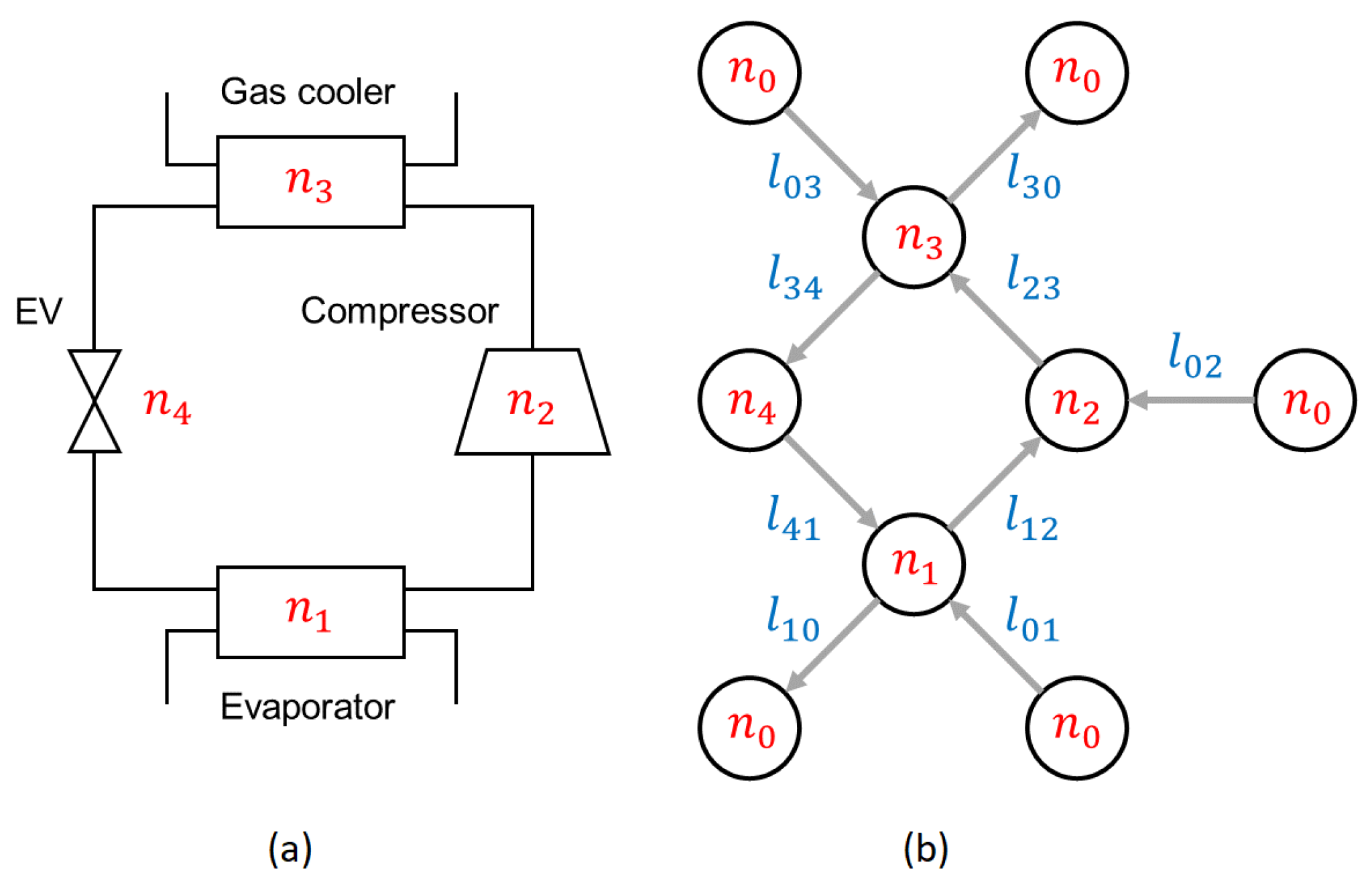
The way in which each component in the heat pump system is represented using control volume (CV) regions is discussed in this section. The specific methodology used to solve for the key driving parameters present in the derived component-specific conservation and characteristic equations is also discussed. The modeling discussion proceeds in the chronological order of evaporator first, compressor second, gas cooler third and concludes with the modeling of the electronic expansion valve component.

Appendix A.1. Evaporator

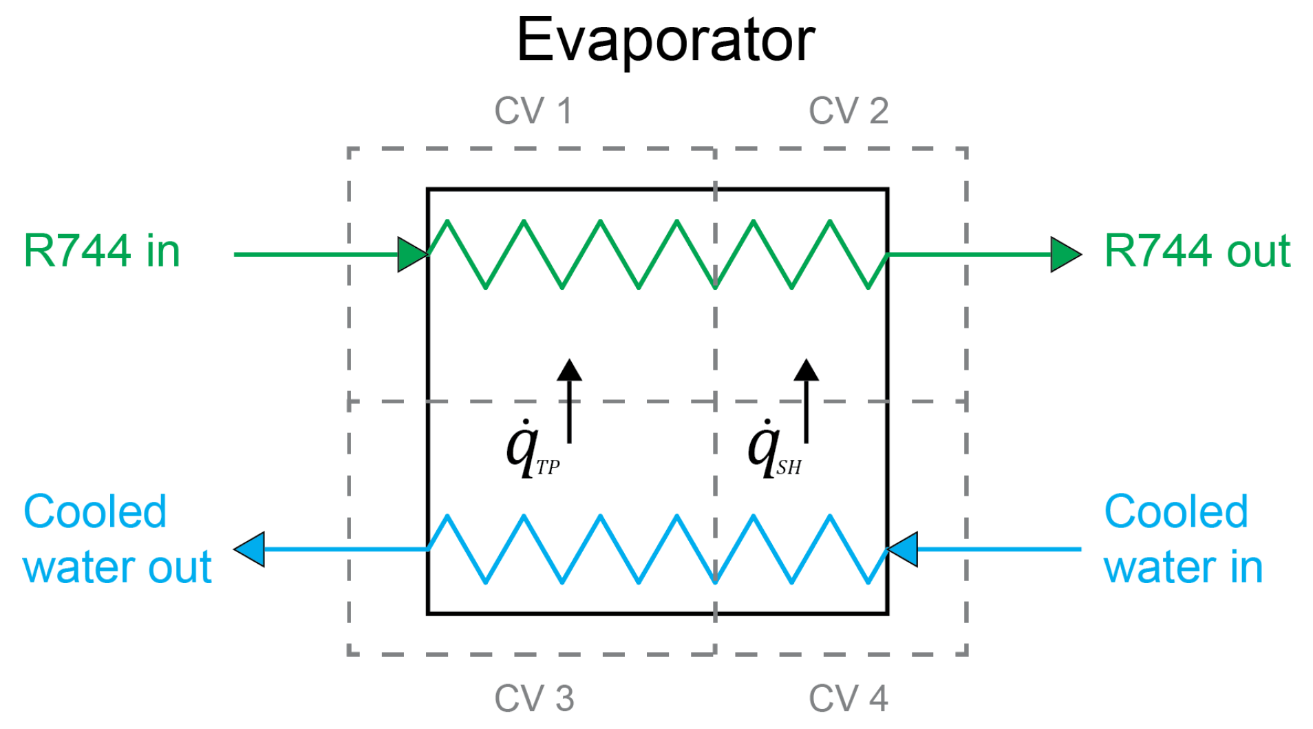
The evaporator component is divided into two CVs on the refrigerant side and two corresponding CVs on the cooled water side, as illustrated in Figure A1.
Figure A1. Evaporator component divided into four control volume regions.
Energies 13 01783 g0a1
It is assumed that the mass flow rate, temperature, and pressure are known at the inlet of the R744 side of the evaporator. The amount of superheating is also known at the outlet of the evaporator component and is controlled by the EV orifice opening percentage. It is also assumed that the water side of the evaporator, the volumetric flow rate delivered by the pump, the inlet temperature, and the pressure of the water are known. The conservation of mass balance for the R744 side of the evaporator is given by:
{ m ˙ i n | E } R 744 = { m ˙ o u t | E } R 744 .
The conservation of mass for the water side of the evaporator is described by:
{ ρ i n | E · q ˙ i n | E } w = { ρ o u t | E · q ˙ o u t | E } w .
The conservation of momentum for the R744 side of the evaporator is as follows:
{ P 0 i n | E } R 744 = { P 0 o u t | E } R 744 + Δ P 0 L | E .
The total pressure drop, Δ P 0 L | E , that the R744 undergoes along the length of the evaporator is the sum of the total pressure drop that occurs in the evaporator’s two-phase region and the total pressure drop that occurs in the preceding superheating region. The total pressure drop that the R744 undergoes in the two-phase region, Δ P 0 L | T P , is modeled using the Friedel method [41].
In the Friedel method the total lengthwise two-phase pressure drop, Δ P 0 L | T P , is a function of the pressure drop that would occur in the two-phase region if the whole pipe was filled with only a liquid, Δ P , multiplied by the squared two-phase Friedel multiplier, Φ f r t p . The superscript t p refers to a two-phase working fluid. The Friedel method is expressed mathematically as:
Δ P 0 L | T P = Δ P × Φ f r t p .
The R744 liquid-based pressure drop is expressed as:
Δ P = 4 f l L T P D H , R 744 m v e l t p 1 2 ρ b l c 1 c 2 ,
where f l is the liquid-based friction factor, L T P is the length of the two-phase region in the evaporator, D H , R 744 is hydraulic diameter of the homogeneous R744 flow, m v e l t p is the mass velocity of the two-phase R744 mixture, and ρ b l is the liquid-based bulk density in the two-phase region. The liquid-based friction factor is calculated by use of the Blasius correlation [41,42]:
f l = 0.079 R e b l 0.25 ,
where R e b l is the bulk dimensionless liquid-based Reynolds number in the two-phase region. The mass velocity of the R744 two-phase flow is simply the total R744 mass flow through the evaporator divided by the free flow area of the inner evaporator tube:
m v e l t p = m ˙ R 744 π 4 D i i 2 .
After the liquid-based pressure drop has been determined; the two-phase Friedel multiplier is required to calculate the total two-phase pressure drop with relation to the liquid-based pressure drop in the two-phase region. The Friedel multiplier is expressed as a function of five dimensionless parameters as:
ϕ f r t p = E + 3.24 ( F · H ) F r H 0.045 + W e l 0.035 .
The first dimensionless parameter is defined as:
E = ( 1 x b ) 2 + ( x b ) 2 ρ l f v ρ v f l ,
where x b is the bulk quality dryness fraction of the two-phase region and f v is the bulk vapor-based friction factor. The second dimensionless parameter is defined as:
F = x b 0.78 × ( 1 x b ) 0.224 .
The third dimensionless parameter is defined as:
H = ρ l ρ v 0.91 μ v μ l 0.19 1 μ v μ l 0.7
The homogeneous Froude number is defined as:
F r H = m v e l 2 g · D i i · ρ b H 2 ,
where g is the local gravitational acceleration at the physical location of the heat pump system and ρ b H is the bulk homogeneous density of the two-phase flow in the two-phase region. The liquid-based Weber number is defined as:
W e l = m v e l 2 · D i i σ b · ρ b H ,
where ρ b is the surface tension at the bulk conditions in the two-phase flow region.
The superheat region follows the two-phase region in the evaporator. The total pressure drop that occurs in the superheat region is expressed as:
Δ P 0 L | S H = f S H L S H D H , R 744 1 2 ρ b | S H C b | S H 2 c 1 c 2 .
The Darcy friction factor for the superheat region is determined using the built-in EES ® MoodyChart function as follows:
f S H = M o o d y C h a r t R e b | S H , e s s D H , R 744 .
The total pressure drop on the R744 side of the evaporator is then the sum of the total pressure in the two-phase region and the total pressure drop in the superheat region:
Δ P 0 L | E = Δ P 0 L | T P + Δ P 0 L | S H .
The length of the two-phase region added to the length of the superheating region must equate to the total length of the tube in the evaporator component:
L T P + L S H = L E .
The focus of the simulation is on the modeling of the refrigerant side of the heat pump system. The total pressure drop on the water side of the evaporator is assumed to be negligible. Under this assumption the conservation of momentum for the water side of the evaporator is simply:
{ P 0 i n | E } w = { P 0 o u t | E } w .
The conservation of energy for the R744 side of the evaporator is:
{ m ˙ i n h 0 | i n } R 744 + Q E = { m ˙ o u t h 0 | o u t } R 744 .
The total heat absorbed by the R744 during the evaporation process is equal to the total heat absorbed in the two-phase region and in the superheat region within the evaporator:
Q E = Q T P + Q S H .
The total enthalpy at the start of the superheat region can easily be calculated when the total pressure drop in the two-phase region is known. The total enthalpy at the start of the superheat region may thus be calculated in EES ® as follows:
{ h 0 | i n } S H = f P = { P 0 | i n } T P Δ P 0 L | T P , x = 1 .
Once the total enthalpy at the start of the superheat region is known, the heat transfer in the two-phase region can be calculated by performing an energy balance for CV 1 as in Figure A1. The result is:
Q T P = m ˙ R 744 { h 0 | i n } S H { h 0 | i n } T P .
Since the amount of superheat at the outlet of the evaporator component is controlled by the EEV operation, the heat transfer in the superheat region is calculated from the single-phase relation:
Q S H = m ˙ R 744 × C p b | S H × Δ T S H .
The heat absorbed by the R744 during the evaporation process is supplied from the cooled water stream. The conservation of energy for the water side of the evaporator is thus given by:
m ˙ i n h 0 | i n w = m ˙ o u t h 0 | o u t w + Q E .
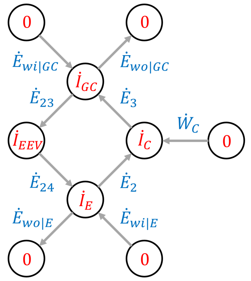
The exergy analysis of the evaporator is performed over the entire evaporator component. The exergy analysis thus considers all four CV regions that encapsulate the evaporator interactions simultaneously. The exergy balance over the entire evaporator is thus given by:
X ˙ i n R 744 + X ˙ i n w = X ˙ o u t R 744 + X ˙ o u t w + I ˙ E .

Appendix A.2. Compressor

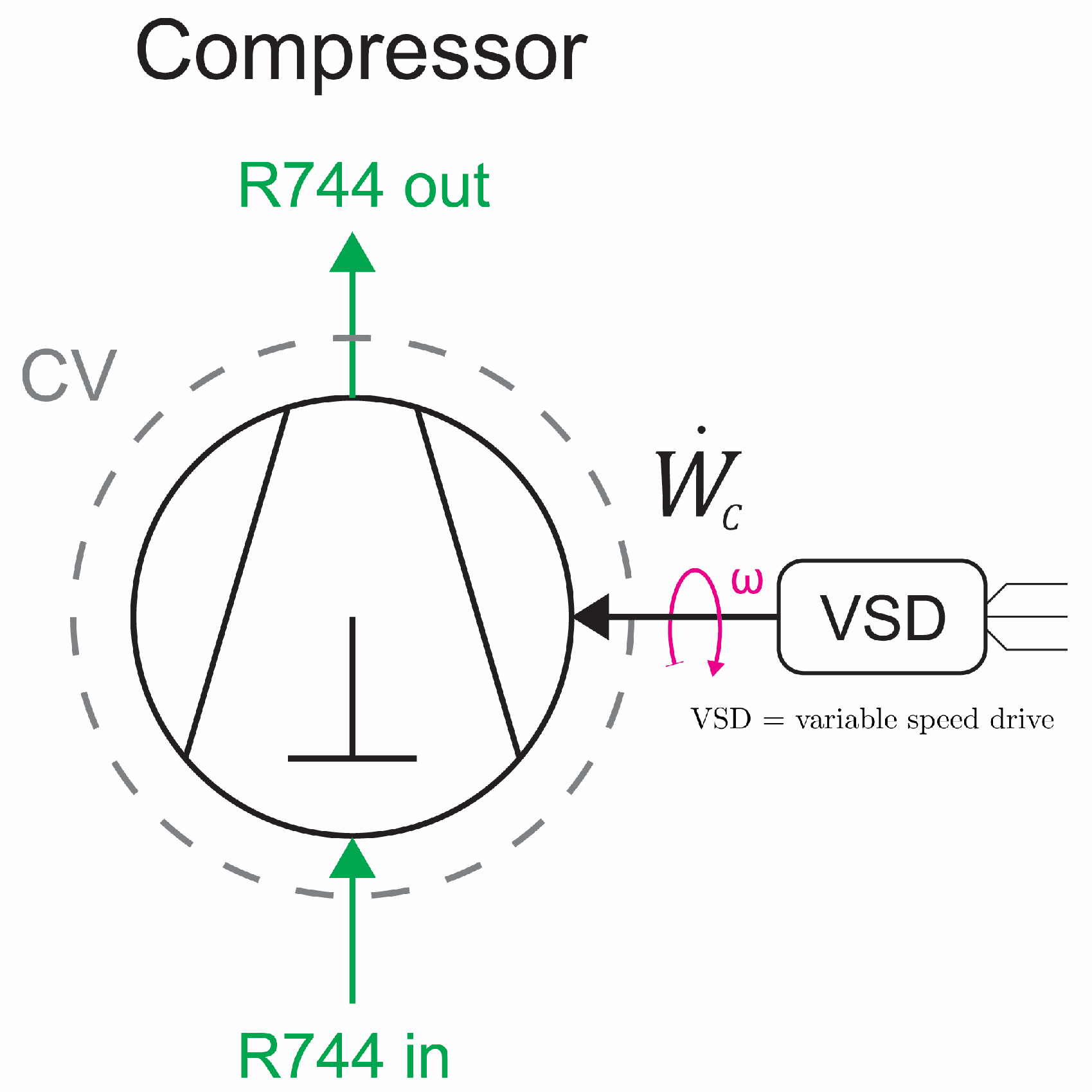
The compressor component is represented using one CV. The compressor component with its CV indicated as illustrated in Figure A2.
Figure A2. Compressor component with its CV.
Energies 13 01783 g0a2
The compressor only has carbon dioxide as its interacting fluid with the conservation of mass for the compressor component given by:
m ˙ i n | C R 744 = m ˙ o u t | C R 744 .
The discharge pressure of the R744 after compression is defined by the compressor’s ratio of pressure:
P 0 | o u t R 744 = r P × P 0 | i n R 744 .
The conservation of energy for the compressor is given by:
m ˙ i n h 0 | i n R 744 + W ˙ C = m ˙ o u t h 0 | o u t R 744 ,
where W ˙ C is the power absorbed by the compressor during the compression of the carbon dioxide gas. The compressor power drawn is the key parameter required to solve for the output flow energy delivered by the compressor. The compressor power drawn is calculated from the compressor’s isentropic efficiency:
W ˙ C = W ˙ i s e n η i s e n ,
where W ˙ i s e n is the power the compressor would draw in an ideal imaginary isentropic compression process between the same inlet and outlet thermo-physical conditions and η i s e n is the isentropic efficiency of the compressor with a value in the range of zero to one. The ratio of pressure across the compressor will be expressed as a function of the isentropic efficiency of the compressor at various operating conditions. 
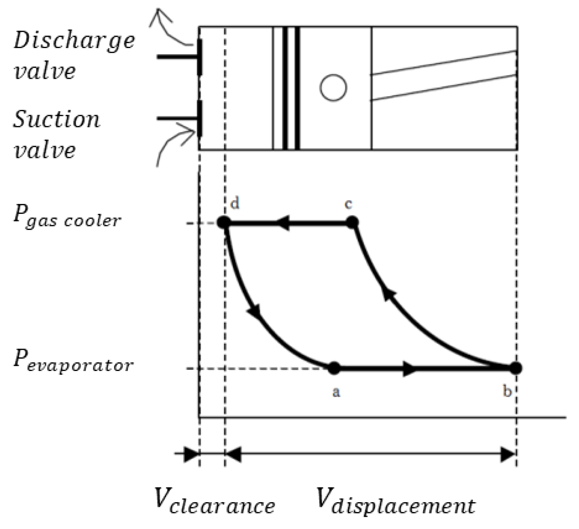
Figure A3 illustrates the pressure-volume behavior of the refrigerant through the compression process inside the compression chamber of a reciprocating compressor.
Four different stages are defined in the cyclic up-and-down movement performed by the compressor’s pistons. At point, a in Figure A3, the suction valve opens during the movement of the piston and low-pressure refrigerant flows into the compression chamber. The piston continues to move and draw in refrigerant until it reaches its bottom dead center (BDC) as indicated by point b in Figure A3. At point b the suction valve closes and the piston starts moving in the opposite direction, compressing the refrigerant. The compression action is illustrated in Figure A3 by the curved line that connects point b and c. At point c the refrigerant reaches a high enough pressure to open the compression chamber’s discharge valve. The refrigerant is pushed out of the compression chamber by the motion of the piston as it moves from point c to its top dead center (TDC) as indicated by point d. The discharge valve closes after the piston has reached point d. The pressure inside the compression chamber is lowered from point d to a as the piston moves from its TDC back towards its BDC. After the piston reaches point a, the process starts anew.
Figure A3. P-V behavior of the refrigerant inside a reciprocating compressor’s piston chamber.
Energies 13 01783 g0a3
The expression to determine the specific work required per piston to compress the refrigerant from the evaporating pressure to the gas cooler pressure is given by:
W c y l = k a v g k a v g 1 P b ν b r P k a v g 1 k a v g 1 1 c 2 ,
where k a v g is the average heat capacity ratio between the compressor’s discharge and suction side, v b is the specific volume of the refrigerant at point b in Figure A3, and r P is the pressure ratio over the compressor during steady-state operation. The total specific work required by the compressor during steady operation is then the specific work required per piston times the number of pistons that compress the refrigerant:
W s p e c = W c y l · # c y l ,
where # c y l is the number of compression cylinders that compress the refrigerant at any given instance during steady-state compressor operation.
The isentropic efficiency of the compressor may thus be simulated by taking the theoretical specific isentropic work required by the compressor at the same operating conditions and dividing it by the calculated actual specific work required by the compressor:
η s i m = W i s e n W s p e c .
The accuracy of (A32) can be improved by including two constants into the equation that were determined from test bench data. The improved equation for the isentropic efficiency of the compressor is given by:
η s i m = W i s e n a 1 · W s p e c b 1 ,
where a 1 = 1.629497 and b 1 = 0.869919 . The isentropic efficiency of the compressor is assumed to be known in this study and its value is used as an input parameter in the simulation of the heat pump system. This approach may be used to implicitly determine the ratio of pressure over the compressor when the isentropic efficiency of the compressor is known, as is evident from inspection of (A30).
The exergy balance for the compressor is given by:
X ˙ i n R 744 + W ˙ C = X ˙ o u t R 744 + I ˙ C .

Appendix A.3. Gas Cooler

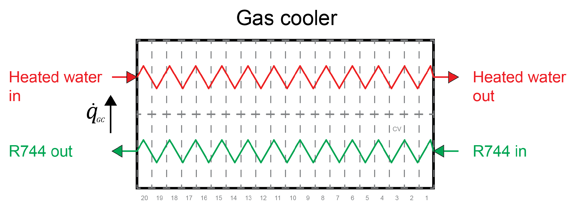
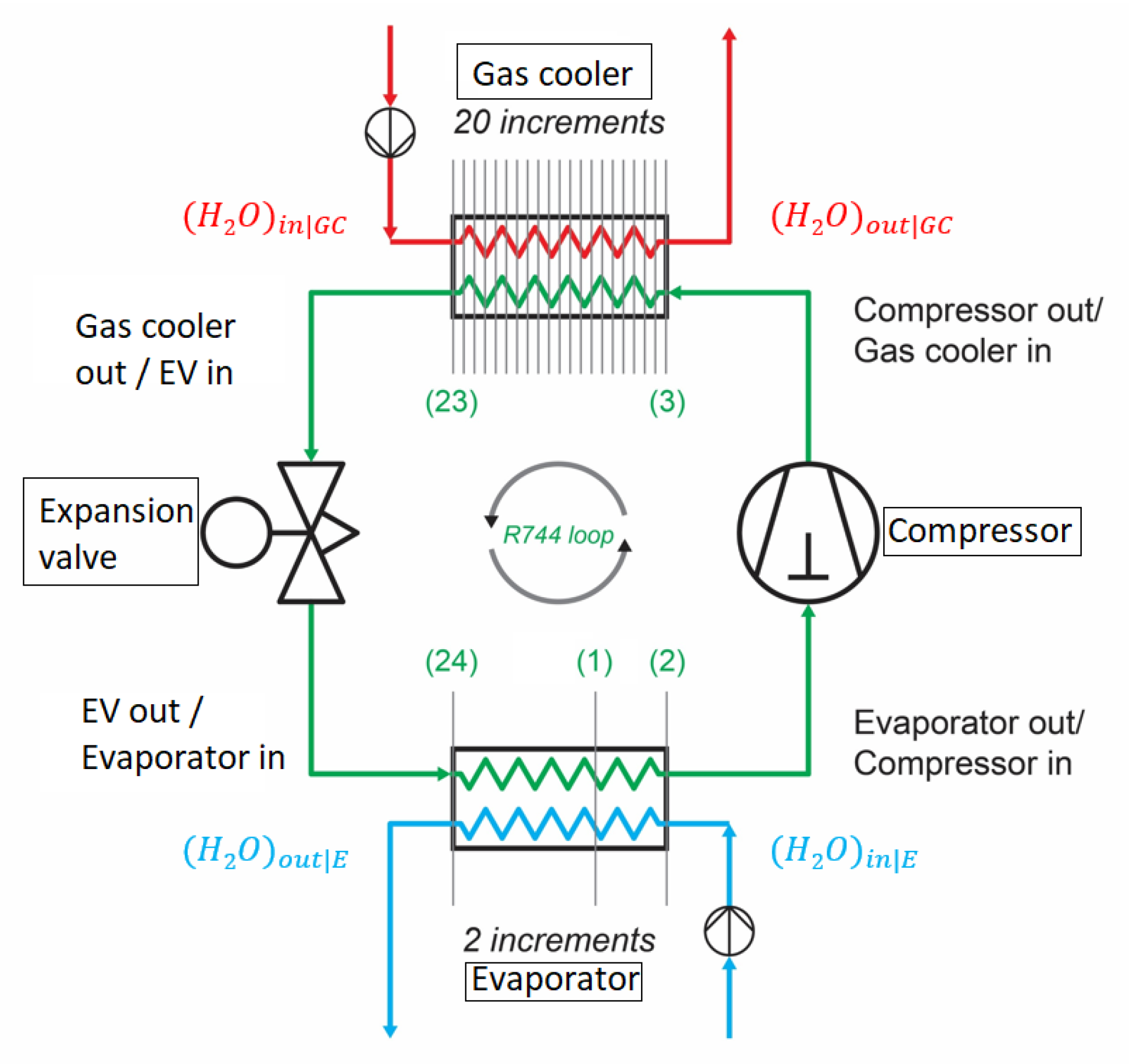
The gas cooler is divided into 20 control volumes on the refrigerant side and 20 corresponding control volumes on the heated water side. This was done to accurately calculate the heat transfer in the gas cooler component using the ε -
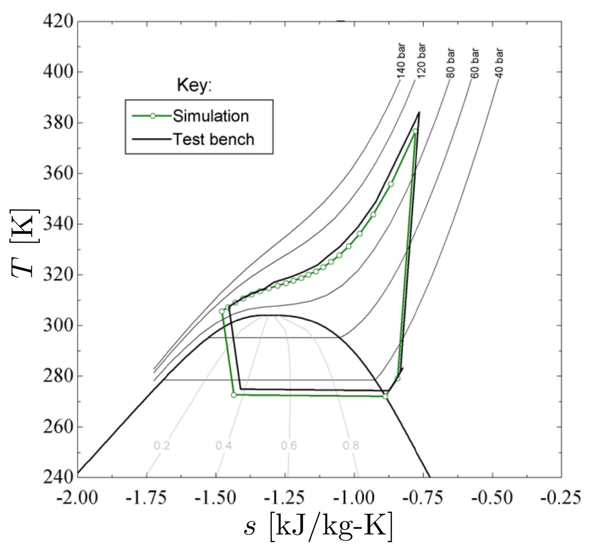
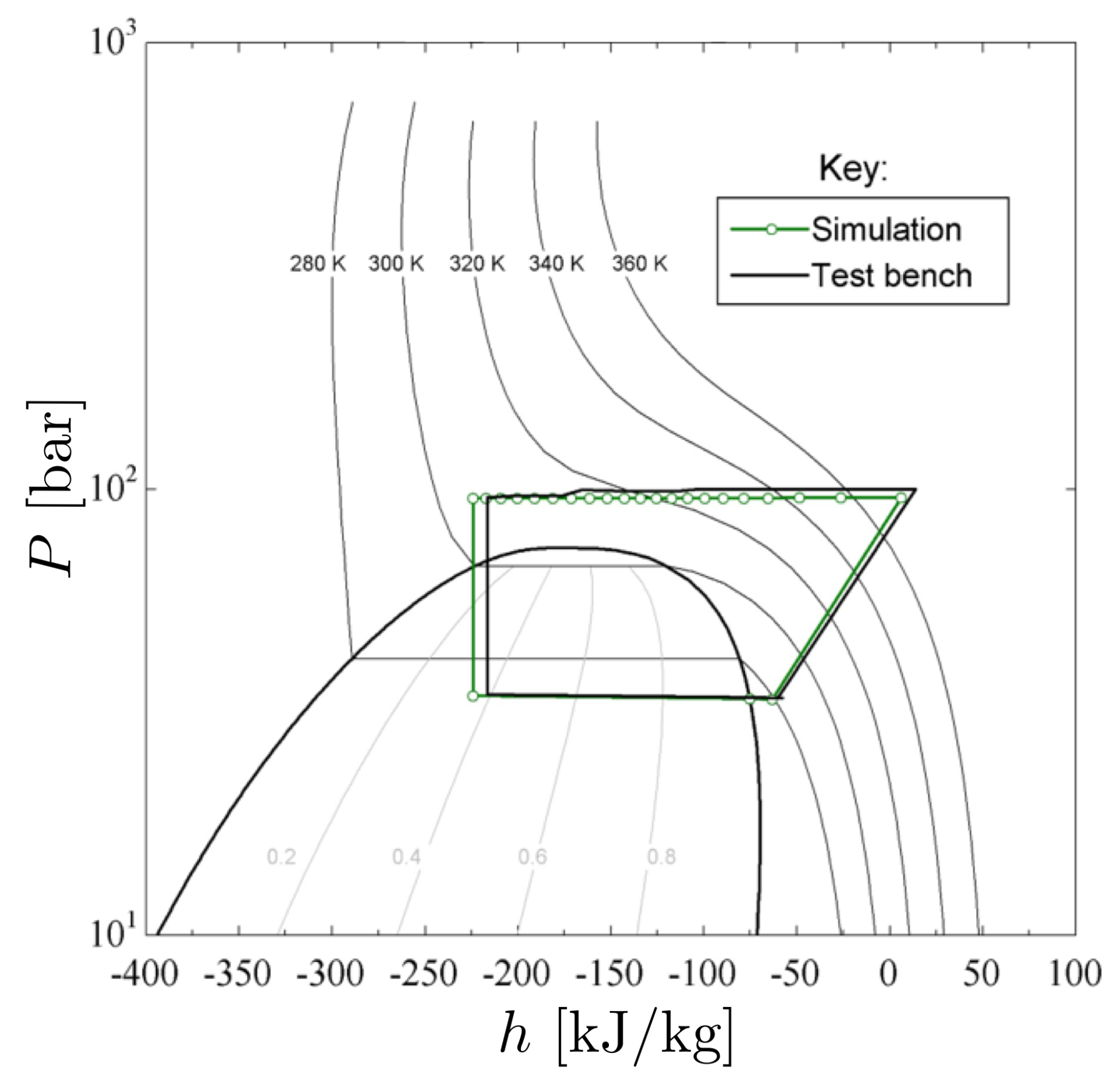
NTU method. The segmentation is also beneficial when plotting the supercritical heat rejection curve of the refrigerant on a T-s diagram. The gas cooler component with its control volume regions is illustrated in Figure A4.
Figure A4. Gas cooler component divided into control volume regions.
Energies 13 01783 g0a4
It is assumed that the mass flow rate, temperature, and pressure are known at the inlet of the R744 side of the gas cooler. It is also assumed that the volumetric flow rate, inlet temperature and pressure are known on the water side. The conservation of mass balance on the R744 side of the gas cooler is given by:
m ˙ i n | G C R 744 = m ˙ o u t | G C R 744 .
The conservation of mass balance on the water side of the gas cooler is:
ρ i n | G C q ˙ i n | G C w = ρ o u t | G C q ˙ o u t | G C w
The density of the water, ρ w , [kg/m 3 ] and q ˙ G C the volumetric flow rate of the heated water through the gas cooler has a unit [m 3 /s]. The conservation of momentum for the R744 side of the gas cooler is
P 0 i n | G C R 744 = P 0 o u t | G C R 744 + Δ P 0 L | G C ,
where Δ P 0 L | G C is the total pressure drop of the R744 along the length of the gas cooler. The total pressure drop is a function of flow channel friction, the total coil length, the hydraulic diameter, and the thermo-physical properties of R744 as it flows through the gas cooler. The total pressure drop on the R744 side of the gas cooler is equal to the sum of the pressure drop over each segment on the refrigerant side. The pressure drop per increment on the refrigerant side is given by:
Δ P 0 L | i n c = f W L i n c D H , R 744 1 2 ρ b g V b g 2 c 1 c 2 ,
where f W is the friction factor correlation by Wang et al. [43] for the prediction of supercritical carbon dioxide pressure drop in the turbulent flow regime, L i n c is the length of the increment, D H , R 744 is the hydraulic diameter, ρ b g is the bulk density per increment, and V b g is the bulk velocity per increment. The friction factor correlation by Wang et al. is given by:
1 s q r t f W = 2.34 · log e s s 1.72 D H , R 744 9.26 R e b g · log e s s 29.36 D H , R 744 0.95 + 18.35 R e b g 1.108 .
The parameter e s s is the surface roughness of the inner gas cooler tube material and R e b g is the dimensionless bulk Reynolds number of the R744 per increment. The correlation by Wang et al. has a valid Reynolds number range of: 3400 < R e b g < 2 × 10 6 . The pressure drop on the water side of the gas cooler is assumed to be negligible. Under this assumption the conservation of momentum equation for the entire water side of the gas cooler is given by:
P 0 i n | G C w = P 0 o u t | G C w .
The conservation of energy for the R744 side of the gas cooler is:
m ˙ i n h 0 | i n R 744 = Q G C + m ˙ o u t h 0 | o u t R 744 .
The energy extracted from the R744 side of the gas cooler during the cooling process is absorbed by the heated water side. The conservation of energy for the water side of the gas cooler is described by:
m ˙ i n h 0 | i n w + Q G C = m ˙ o u t h 0 | o u t w ,
where Q G C is the total heat transfer that takes place from the R744 to the water stream. The total heat transfer is the sum of the heat transfer per increment on the R744 side of the gas cooler. The heat transfer per increment will be solved by using the ε -NTU method. The heat transfer per increment is given by:
Q i n c = Q max | i n c × ε i n c ,
where Q m a x | i n c is the maximum theoretical heat transfer possible per increment and ε i n c is the effectiveness of the gas cooler in transferring heat per increment in the range of 0.1. The maximum heat transfer per increment is given by:
Q m a x | i n c = C m i n Δ T m a x | i n c ,
where C m i n is the minimum heat capacity rate between the two interacting fluid streams and Δ T m a x is the temperature difference between the R744 and water, at their respective inlets, per increment. The effectiveness per increment for a counter-flow tube-in-tube type of heat exchanger is defined by Bergman et al. [44] as:
ε i n c = 1 exp N T U 1 c r 1 c r · exp N T U 1 c r i n c ,
where NTU is the dimensionless number of transfer units per segment of the gas cooler and c r is the dimensionless capacity ratio of the interacting fluids. Equation (A45) is valid for all possible values of the capacity ratio that are smaller than one. The capacity ratio is expressed as the ratio of the minimum to maximum heat capacity rates of the interacting heat exchanger fluids per increment:
c r i n c = H C R m i n H C R m a x i n c = m ˙ c p b m i n m ˙ c p b m a x i n c ,
where c p b is the bulk specific heat capacity at constant pressure per increment for a given fluid stream. The number of transfer units per gas cooler increment is given by:
N T U i n c = U A s H C R m i n i n c ,
where U is the overall heat transfer coefficient per gas cooler increment and A s is the heat transfer surface area per increment. It is assumed that there is no possibility of fouling build-up on the R744 side of the gas cooler while it is possible for the water side to foul. Furthermore, it is also assumed that the gas cooler is well insulated on the outside of the outer tube such that there is no possibility of heat loss to the environment. Under these assumptions the product of the overall heat transfer coefficient with the heat transfer surface area per gas cooler increment may be expressed in terms of thermal resistance as [45]:
1 U A s i n c = 1 ( h c o n v A ) R 744 + ln D i o D i i 2 π k t u b e L i n c + F F i o A w + 1 ( h c o n v A ) w i n c .
The first term in (A48) is the total thermal resistance per gas cooler increment, the second term is the convection thermal resistance on the R744 side and the third term is the conduction thermal resistance per increment. The fourth term is the fouling resistance on the heated water side and the fifth term is the convection resistance of the heated water side on the gas cooler.
The Dittus-Boelter correlation [46] is used to solve for the convection coefficient, h c o n v , on both the R744 and the water side of the gas cooler. Although correlations exist that can predict the convection coefficient of supercritical R744 with higher accuracies such as those investigated by Venter [47], the study by van Eldik et al. [38] showed that the Dittus-Boelter correlation shows an excellent fit (for larger diameter tubes) with experimental data over a wider range of Reynolds number values. The study by [38] also concluded that the Dittus-Boelter correlation remains relatively stable when used to calculate convection coefficients based on thermo-physical conditions in the pseudo-critical region of carbon dioxide. The convection coefficient per gas cooler increment while implementing the Dittus-Boelter correlation is expressed as:
h c o n v i n c = C F 0.023 k b D H R e b 0.8 P r b n ,
where C F is a correlation factor specifically fitted to the specific test bench system to further increase the accuracy of the Dittus-Boelter correlation, k b is the bulk conduction heat transfer coefficient of the fluid, P r b is the bulk dimensionless Prandtl number of the fluid per gas cooler increment and n is a power set to 0.3 if the fluid considered is cooled or set to 0.4 if the fluid is heated. The CF factor for the experimental data used in this study is 2.294 [-]. The C F factor is included to make the prediction of heat transfer values associated with the test bench system as accurate as possible. The CF factor reported here is only valid for this study. The CF factor used here is an average of all the individual factors determined by setting the simulation results equal to the experimental results. The CF factor is thus a form of direct numerical fitting of the simulation to the test bench results. The exergy analysis of the gas cooler is done over the entire component. The exergy balance over the entire gas cooler is given:
X ˙ i n R 744 + X ˙ i n w = X ˙ o u t R 744 + X ˙ o u t w + I ˙ G C .

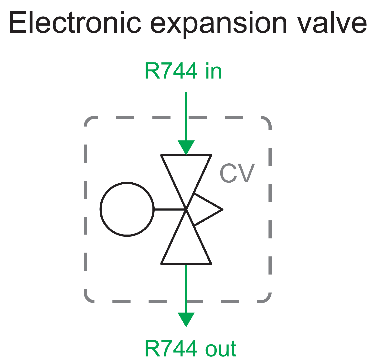
Appendix A.4. Expansion Valve

The EV component is represented with one CV. The EV component with its CV is illustrated in Figure A5.
Figure A5. EV component with its CV region.
Energies 13 01783 g0a5
The EV has only carbon dioxide as its interacting fluid. The conservation of mass for the R744 flowing through the EV component is given by:
m ˙ i n | E V R 744 = m ˙ o u t | E V R 744 .
The EV controls the mass flow rate of the refrigerant through the entire heat pump system. The BITZERTM Software v6.7.0 utility [48] may be used to find the recommended mass flow rate for the BITZERTM type 4JTC-15K (40P) compressor operating at specific working points. The amount of refrigerant that was loaded into the heat pump test bench was done by an operator. The mass flow rate of the refrigerant at various locations throughout the heat pump system may thus not match the mass flow rate recommended by the BITZER
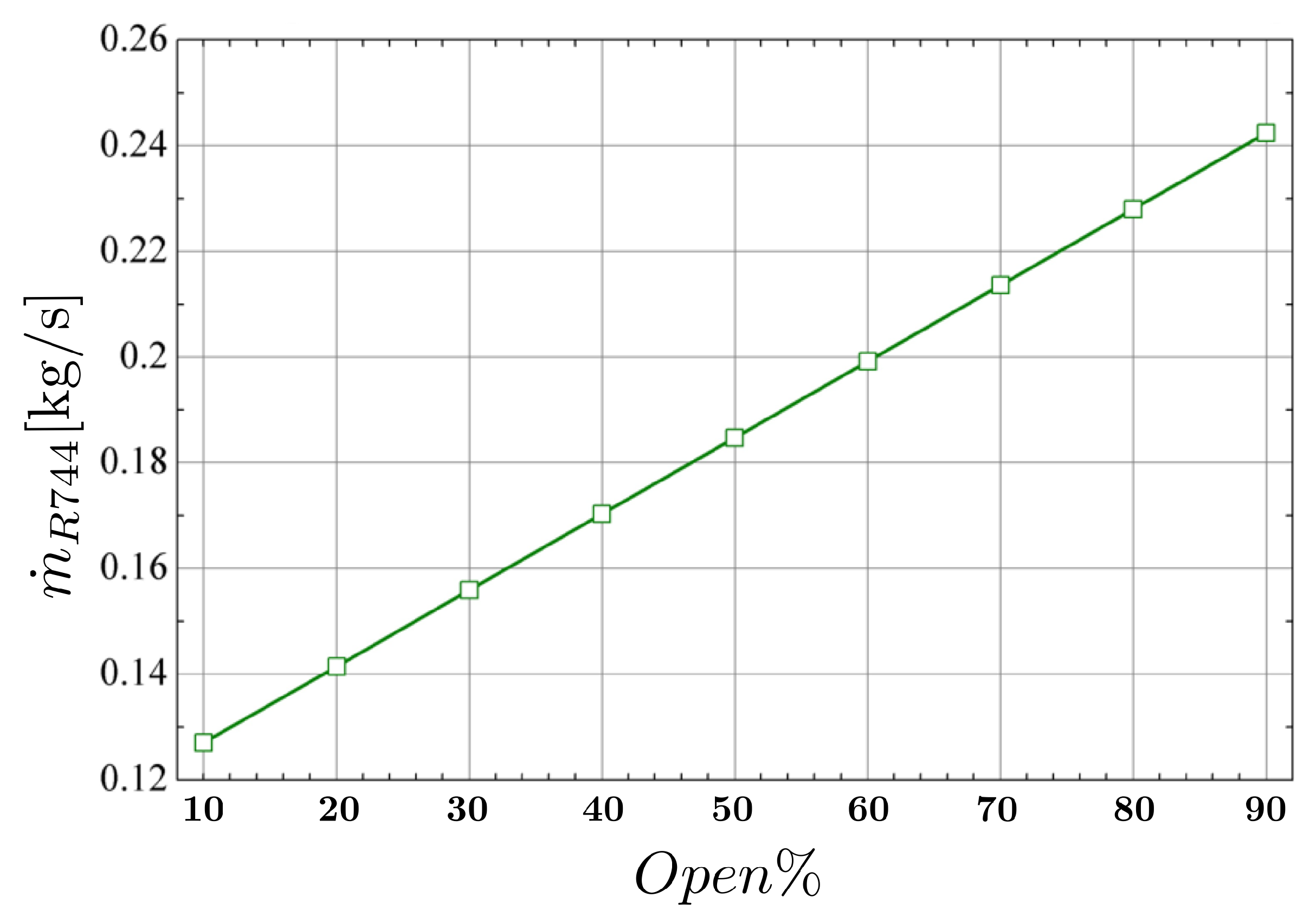
TM Software utility. A better approach is a linear regression fit of the refrigerant mass flow as a function of the EV orifice opening percentage for the actual test bench. The built-in EES® [23] linear regression utility was used to fit the mass flow rate of the refrigerant to the experimental data generated from the heat pump test bench. The fitted linear relation of mass flow as a function of the EV orifice opening is illustrated in Figure A6.
From Figure A6 it should be noted that a decrease in the flow restricting orifice opening area percentage leads to an increase in the mass flow rate of the refrigerant through the entire heat pump system. The specific linear equation that describes the relationship between the refrigerant mass flow rate and EV orifice opening of the line displayed in Figure A6 is:
m ˙ R 744 = 0.1442 100 O p e n % + 0.11262 .
Figure A6. Refrigerant mass flow rate as a function of EV opening.
Energies 13 01783 g0a6
The conservation of momentum for the R744 that undergoes throttling as it passes through the EV is given by:
P 0 i n | E E V R 744 = P 0 o u t | E E V R 744 + Δ P 0 L | E E V .
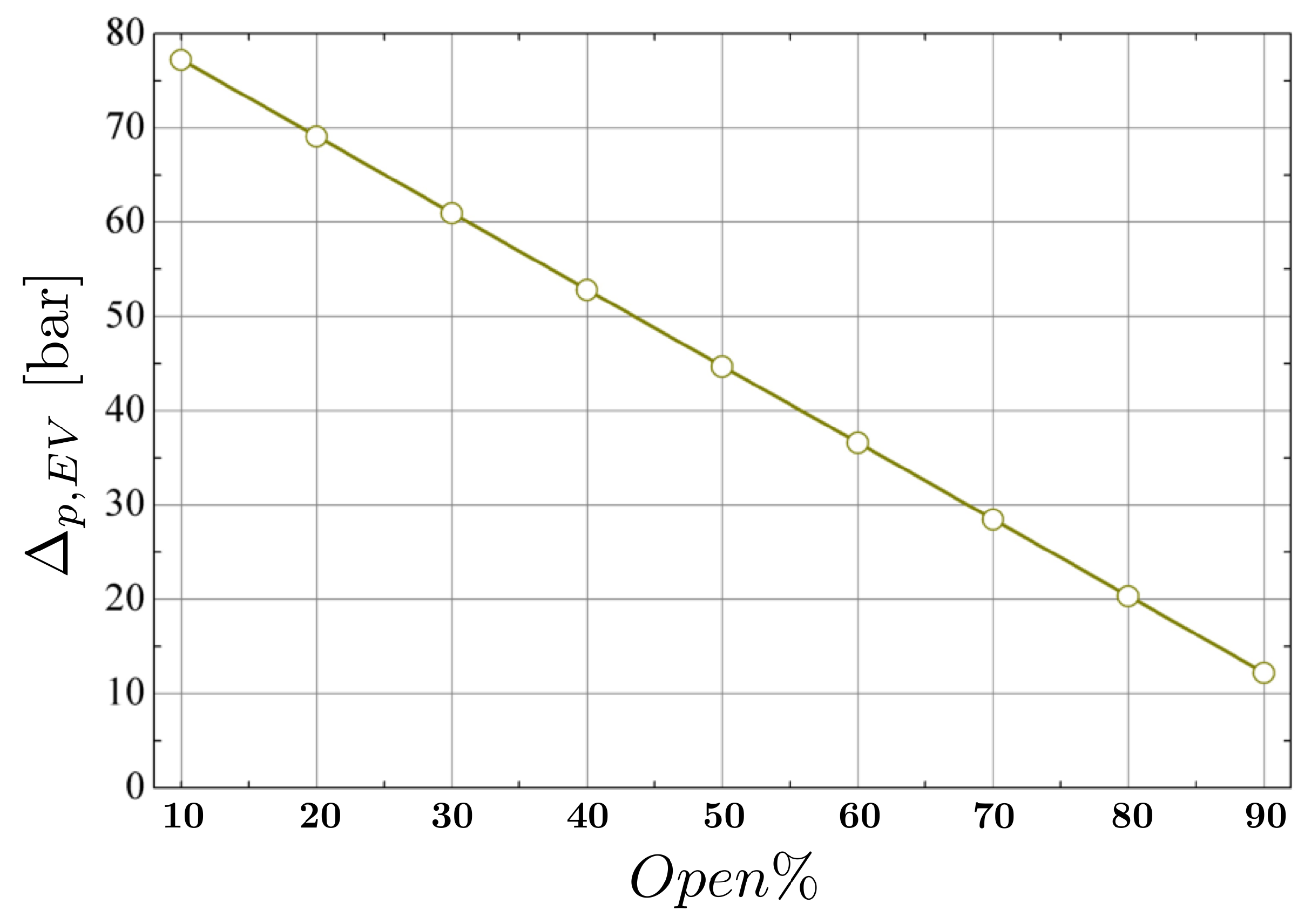
Since the physical dimensions of the internal EV mechanisms are not readily available, a new method is required to predict the total pressure drop over the EV component. The static pressure drop over the EV is modeled as an inverse linearly proportional function of the opening percentage of the expansion valve orifice area. The suggested inverse linearly proportional graph of the static pressure drop over the EV as a function of the opening percentage of the expansion valve orifice is illustrated in Figure A7.
Figure A7. Static pressure drop over EV vs EV orifice opening.
Energies 13 01783 g0a7
From Figure A7 it should be noted that the static pressure drop over the expansion valve orifice tends to zero as the valve orifice is increasingly opened. This trend is suited because when the EEV orifice is 100% open it will not offer any resistance to the flow of the refrigerant and the induced pressure drop on the refrigerant will thus be zero. The specific linear equation that describes the line displayed in Figure A7 is:
Δ p , E V = 81.30 100 O p e n % + 85.37 .
Once the static pressure drop over the EV is known, it can easily be converted to total pressure drop by adding the kinetic energy component of total pressure to the static pressure drop value. The throttling of the R744 through the EV is assumed to be an isenthalpic process. Under this assumption the conservation of energy for the EV is simply:
h 0 | i n R 744 = h 0 | o u t R 744 .
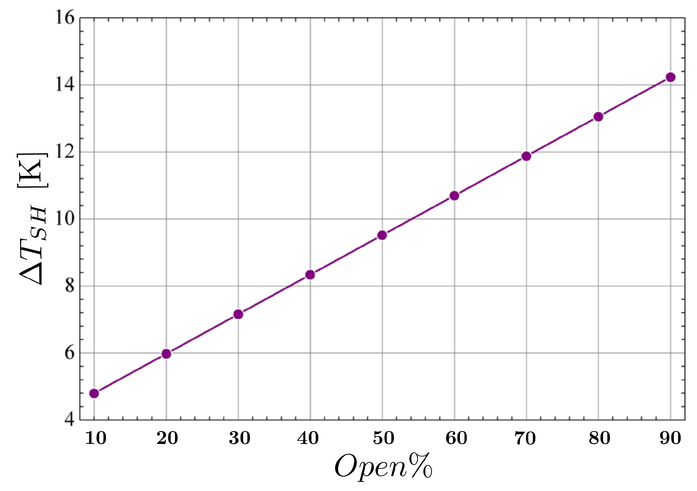
Another important cycle parameter controlled by the EV is the amount of superheating that takes place in the evaporator. A linear equation is also used to describe the amount of superheating as a function of the EV orifice opening. The linear relationship between the amount of evaporator superheating and the EV orifice opening is shown in Figure A8.
Figure A8. Amount of superheating in evaporator vs EV orifice opening.
Energies 13 01783 g0a8
The specific linear equation that describes the line displayed in Figure A8 is:
Δ T S H = 11.8 100 O p e n % + 3.62 .
The exergy balance over the EV is performed over the entire EV CV region. The exergy balance for the EV is given by:
X ˙ i n R 744 = X ˙ o u t R 744 + I ˙ E E V .

References

  1. Zogg, D. Fault Diagnosis for Heat Pump Systems; ETH Zurich: Zurich, Switzerland, 2002. [Google Scholar]
  2. Erb, M.; Hubacher, P.; Eicher, H.; Farner, M. Feldanalyse von WP-Anlagen; Technical Report; Bundesamt für Energie: Bern, Germany, 2000. [Google Scholar]
  3. Conant, A.; Moder, M.; Pira, J.; Proctor, P.; Gebbie, M. Comprehensive Diagnostic and Improvement Tools for HVAC-System Installations in Light Commercial Buildings. 2004. Available online: https://www.proctoreng.com/dnld/Comprehensive_Diagnostic_and_Improvement_Tools_000.pdf (accessed on 21 May 2019).
  4. Rossi, T.M. Unitary Air Conditioner Field Performance. In Proceedings of the International Refrigeration and Air Conditioning Conference at Purdue University, Purdue, IN, USA, 12–15 July 2004; pp. 1–9. [Google Scholar]
  5. Zhao, Y.; Li, T.; Zhang, X.; Zhang, C. Artificial intelligence-based fault detection and diagnosis methods for building energy systems: Advantages, challenges and the future. Renew. Sustain. Energy Rev. 2019, 109, 85–101. [Google Scholar] [CrossRef]
  6. Shi, Z.; O’Brien, W. Development and implementation of automated fault detection and diagnostics for building systems: A review. Autom. Constr. 2019, 104, 215–229. [Google Scholar] [CrossRef]
  7. Kim, W.; Katipamula, S. A review of fault detection and diagnostics methods for building systems. Sci. Technol. Built Environ. 2018, 24, 3–21. [Google Scholar] [CrossRef]
  8. Yoo, Y.J. Fault Detection Method Using Multi-mode Principal Component Analysis Based on Gaussian Mixture Model for Sewage Source Heat Pump System. Int. J. Control Autom. Syst. 2019, 17, 2125–2134. [Google Scholar] [CrossRef]
  9. Chen, Y.; Lan, L. A fault detection technique for air-source heat pump water chiller/heaters. Energy Build. 2009, 41, 881–887. [Google Scholar] [CrossRef]
  10. Kim, M.; Yoon, S.H.; Payne, W.V.; Domanski, P.A. Development of the reference model for a residential heat pump system for cooling mode fault detection and diagnosis. J. Mech. Sci. Technol. 2010, 24, 1481–1489. [Google Scholar] [CrossRef]
  11. Severson, K.; Chaiwatanodom, P.; Braatz, R.D. Perspectives on Process Monitoring of Industrial Systems. IFAC-PapersOnLine 2015, 48, 931–939. [Google Scholar] [CrossRef]
  12. Lemma, T.A. A Hybrid Approach for Power Plant Fault Diagnostics; Springer: Cham, Switzerland, 2018. [Google Scholar]
  13. Van Schoor, G.; Uren, K.R.; van Wyk, M.A.; van Vuuren, P.A.; du Rand, C.P. An energy perspective on modelling, supervision, and control of large-scale industrial systems: Survey and framework. IFAC Proc. Vol. 2014, 47, 6692–6703. [Google Scholar] [CrossRef] [Green Version]
  14. Marais, H.J.; van Schoor, G.; Uren, K.R. An Energy-based approach to condition monitoring of industrial processes. IFAC-PapersOnLine 2015, 48, 772–777. [Google Scholar] [CrossRef]
  15. Uren, K.R.; van Schoor, G. Energy-based visualisation of a counter-flow heat exchanger for the purpose of fault identification. IFAC-PapersOnLine 2016, 49, 19–24. [Google Scholar] [CrossRef]
  16. Marais, H.J.; van Schoor, G.; Uren, K.R. Energy-based Fault Detection for an Autothermal Reformer. IFAC-PapersOnLine 2016, 49, 353–358. [Google Scholar] [CrossRef]
  17. Van Graan, S.; van Schoor, G.; Uren, K. Graph matching as a means to energy-visualisation of a counter-flow heat exchanger for the purpose of fault diagnosis. IFAC-PapersOnLine 2017, 50, 2842–2847. [Google Scholar] [CrossRef]
  18. Uren, K.R.; van Schoor, G.; Auret, L. An energy-attributed graph approach for the purposes of FDI in a heated two-tank system. IFAC-PapersOnLine 2019, 52, 159–164. [Google Scholar] [CrossRef]
  19. Van Schoor, G.; Uren, K. A vision of energy-based visualisation of large scale industrial systems for the purposes of condition monitoring. In Proceedings of the 31st Conference on Condition Monitoring and Diagnostic Engineering Management, Sun City, South Africa, 2–5 July 2018. [Google Scholar]
  20. Marais, H.; van Schoor, G.; Uren, K.R. The merits of exergy-based fault detection in petrochemical processes. J. Process Control 2019, 74, 110–119. [Google Scholar] [CrossRef]
  21. Greyling, S.; Marais, H.; van Schoor, G.; Uren, K.R. Application of Exergy-Based Fault Detection in a Gas-To-Liquids Process Plant. Entropy 2019, 21, 565. [Google Scholar] [CrossRef] [Green Version]
  22. Borgnakke, C.; Sonntag, R. Fundamentals of Thermodynamics; Wiley: Hoboken, NI, USA, 2014. [Google Scholar]
  23. EES Software. 2019. Available online: http://www.fchart.com/ees/ (accessed on 4 April 2019).
  24. Çengel, Y.; Turner, R. Fundamentals of Thermal-Fluid Sciences; McGraw-Hill Series in Mechanical Engineering; McGraw-Hill Higher Education: New York, NY, USA, 2004. [Google Scholar]
  25. Kotas, T. The Exergy Method of Thermal Plant Analysis; Butterowrths: London, UK, 2013. [Google Scholar]
  26. Godsil, C.; Royle, G. Algebraic Graph Theory; Graduate Texts in Mathematics; Springer: New York, NY, USA, 2013. [Google Scholar]
  27. Sourabh, V.; Chowdary, C.R. Peer recommendation in dynamic attributed graphs. Expert Syst. Appl. 2019, 120, 335–345. [Google Scholar] [CrossRef]
  28. Dehmer, M.; Emmert-Streib, F.; Shi, Y. Quantitative Graph Theory: A new branch of graph theory and network science. Inf. Sci. 2017, 418–419, 575–580. [Google Scholar] [CrossRef] [Green Version]
  29. Rahman, M. Basic Graph Theory; Undergraduate Topics in Computer Science; Springer International Publishing: Cham, Switzerland, 2017. [Google Scholar]
  30. Balakrishnan, R.; Ranganathan, K. A Textbook of Graph Theory; Universitext; Springer: New York, NY, USA, 2012. [Google Scholar]
  31. De la Fuente, M. 5th EN/ICE Automation Seminar: Fault Detection Techniques in the Process Industry. 2015. Available online: https://indico.cern.ch/event/459867/attachments/1187105/1721587/FDI_CERN.pdf (accessed on 10 April 2019).
  32. Mishra, C.; Samantaray, A.; Chakraborty, G. Ball bearing defect models: A study of simulated and experimental fault signatures. J. Sound Vib. 2017, 400, 86–112. [Google Scholar] [CrossRef]
  33. Jouili, S.; Mili, I.; Tabbone, S. Attributed graph matching using local descriptions. In Proceedings of the 11th International Conference on Advanced Concepts for Intelligent Vision Systems, Bordeaux, France, 28 September–2 October 2009; pp. 89–99. [Google Scholar]
  34. Wilson, D.R.; Martinez, T.R. Improved heterogeneous distance functions. J. Artif. Intell. Res. 1997, 6, 1–34. [Google Scholar] [CrossRef]
  35. Lay, D.; Lay, S.; McDonald, J. Linear Algebra and Its Applications; Pearson: London, UK, 2016. [Google Scholar]
  36. Boahen, S.; Lee, K.H.; Choi, J.M. Refrigerant Charge Fault Detection and Diagnosis Algorithm for Water-to-Water Heat Pump Unit. Energies 2019, 12, 545. [Google Scholar] [CrossRef] [Green Version]
  37. Rogers, A.; Guo, F.; Rasmussen, B. A review of fault detection and diagnosis methods for residential air conditioning systems. Build. Environ. 2019, 161, 106236. [Google Scholar] [CrossRef]
  38. Van Eldik, M.; Harris, P.M.; Kaiser, W.H.; Rousseau, P.G. Theoretical And Experimental Analysis Of Supercritical Carbon Dioxide Cooling. In Proceedings of the 15th International Refrigeration and Air Conditioning Conference at Purdue University, Purdue, IN, USA, 14–17 July 2014. [Google Scholar]
  39. Cho, C.W.; Lee, H.S.; Won, J.P.; Lee, M.Y. Measurement and evaluation of heating performance of heat pump systems using wasted heat from electric devices for an electric bus. Energies 2012, 5, 658–669. [Google Scholar] [CrossRef] [Green Version]
  40. Zhang, Z.; Dong, X.; Ren, Z.; Lai, T.; Hou, Y. Influence of refrigerant charge amount and EEV opening on the performance of a transcritical CO2 heat pump water heater. Energies 2017, 10, 1521. [Google Scholar] [CrossRef] [Green Version]
  41. Thome, J.R. Chapter Enhanced heat transfer design methods for tubular heat exchangers. In Engineering Data Book III; PP Publico Publications: Essen, Germany, 2016; pp. 340–341. [Google Scholar]
  42. Blasius, H. Das Aehnlichkeitsgesetz bei Reibungsvorgängen in Flüssigkeiten. In Mitteilungen über Forschungsarbeiten auf dem Gebiete des Ingenieurwesens: Insbesondere aus den Laboratorien der Technischen Hochschulen; Springer: Berlin/Heidelberg, Germany, 1913; pp. 1–41. [Google Scholar] [CrossRef] [Green Version]
  43. Wang, Z.; Sun, B.; Wang, J.; Hou, L. Experimental study on the friction coefficient of supercritical carbon dioxide in pipes. Int. J. Greenh. Gas Control 2014, 25, 151–161. [Google Scholar] [CrossRef]
  44. Bergman, T.L.; Incropera, F.P.; DeWitt, D.P.; Lavine, A.S. Fundamentals of Heat and Mass Transfer, 7th ed.; John Wiley & Sons: Hoboken, NJ, USA, 2011. [Google Scholar]
  45. Cengel, Y. Heat and Mass Transfer: Fundamentals and Applications, 5th ed.; McGraw-Hill Higher Education: New York, NY, USA, 2015. [Google Scholar]
  46. Dittus, F.; Boelter, L. University of California publications on engineering. Univ. Calif. Publ. Eng. 1930, 2, 371. [Google Scholar]
  47. Venter, P.v.Z. A Supercritical R-744 Heat Transfer Simulation Implementing Various Nusselt Number Correlations. Master’s Thesis, North-West University, Potchefstroom, South Africa, 2010. [Google Scholar]
  48. BITZER Software 6.7.0 rev1921. 2018. Available online: https://www.bitzer.de/websoftware/ (accessed on 20 March 2018).
Figure 1. Illustration of the transcritical heat pump system with its cyclic points and components [22].
Energies 13 01783 g001
Figure 2. Transcritical heat pump refrigerant loop on a T-s diagram.
Energies 13 01783 g002
Figure 3. Heat pump test facility: (a) from front, (b) from back.
Energies 13 01783 g003
Figure 4. T-s diagram with overlaid experimental and simulated refrigerant cycle (30% EV orifice opening).
Energies 13 01783 g004
Figure 5. Log. P-h diagram with overlaid experimental and simulated refrigerant cycle (30% EV orifice opening).
Energies 13 01783 g005
Figure 6. An example illustration of a linear graph [30].
Energies 13 01783 g006
Figure 7. An attributed graph representation of the heat pump system: (a) schematic representation of the heat pump system, (b) graph representation.
Energies 13 01783 g007
Figure 8. Heat pump graph representation with assigned attribute symbols.
Energies 13 01783 g008
Figure 9. Flowchart of the procedure to determine the entries of the elements in the fault signatures.
Energies 13 01783 g009
Table 1. Heat pump system component list.
NumberDescriptionFunction
1Electrical distribution boardElectricity supply to components
2Danfoss™ PLCData acquisition from sensors
3Danfoss™ VSD interfaceFrequency control of compressor
4Gas coolerCooling of carbon dioxide gas/heating water
5EvaporatorEvaporation and superheating of
carbon dioxide gas/cooling water
6Danfoss™ motor-operatedInstigates phase change of carbon
expansion valvedioxide into a two-phase mixture
7BITZER™ semi-hermeticCirculates the carbon dioxide
reciprocating type compressorthrough the system
8Example temperature sensorMeasures temperature
9Example pressure sensorMeasures pressure
10Gas cooler water flow rate meterMeasures the volumetric flow rate of
water through the gas cooler
11Evaporator water flow rate meterMeasures the volumetric flow rate of
water through the evaporator
12Gas flow meterMeasures the mass flow rate of
carbon dioxide through the gas loop
13Evaporator centrifugal pumpCirculates the water to be cooled
through the evaporator
14Gas cooler centrifugal pumpCirculates the water to be heated
through the gas cooler
Table 2. System input parameters (30% EV orifice opening).
ParameterValueUnit
Compressor’s isentropic efficiency0.6527[-]
Gas cooler water inlet temperature299.45[K]
Gas cooler water volumetric flow rate16.26[L/min]
EV orifice opening30[%]
Evaporator water inlet temperature313.00[K]
Evaporator water volumetric flow rate16.00[L/min]
Table 3. Key cycle parameters at the 30% EV orifice opening cycle operating point.
ParameterTest Bench ValueSimulated ValuePercentage Deviation
m ˙ R 744 0.1556 [kg/s]0.1559 [kg/s]0.19
Δ T S H 7.20 [K]7.16 [K]0.56
Q ˙ S H 1.818 [kW]1.870 [kW]2.86
W ˙ C 11.50 [kW]10.834 [kW]5.79
Q ˙ G C 35.838 [kW]35.882 [kW]0.12
Q ˙ T P 22.520 [kW]23.183 [kW]2.94
Δ P E E V 61.1 [bar]60.98 [bar]0.20
Table 4. Deviation between simulated and test bench results for 40%, 50%, 60%, and 70% EV orifice openings.
% Deviation
40% EV Orifice50% EV Orifice60% EV Orifice70% EV Orifice
ParameterOpeningOpeningOpeningOpening
m ˙ R 744 0.70.871.631.34
Δ T S H 0.710.212.881.82
Q S H 5.4210.672264.7
W C 6.4510.714.6621.27
Q G C 0.180.2925.1260.13
Q T P 2.923.5655.48155.47
Δ P E E V 1.831.712.172.74
Table 5. Parameters assigned to the graph’s node and link attributes.
Assigned AttributeAttribute DescriptionAttribute SymbolUnit
n 0 Irreversible exergy loss of the reference node0[kW]
n 1 Irreversible exergy loss rate in the evaporator I ˙ E [kW]
n 2 Irreversible exergy loss rate in the compressor I ˙ C [kW]
n 3 Irreversible exergy loss rate in the gas cooler I ˙ G C [kW]
n 4 Irreversible exergy loss rate over the EV I ˙ E V [kW]
l 01 Energy flow rate of the water entering the evaporator E ˙ w i | E [kW]
l 02 The power consumed by the compressor W ˙ C [kW]
l 03 Energy flow rate of the water entering the gas cooler E ˙ w i | G C [kW]
l 10 Energy flow rate of the water leaving the evaporator E ˙ w o | E [kW]
l 12 Refrigerant’s flow energy at cycle point 2 E ˙ 2 [kW]
l 23 Refrigerant’s flow energy at cycle point 3 E ˙ 3 [kW]
l 30 Energy flow rate of the water leaving the gas cooler E ˙ w o | G C [kW]
l 34 Refrigerant’s flow energy at cycle point 23 E ˙ 23 [kW]
l 41 Refrigerant’s flow energy at cycle point 24 E ˙ 24 [kW]
Table 6. Percent deviation of the fluid leakage fault condition.
λ 1 5 377.949.5758.5021.40113.63
v 1 5 163.49267.4292.0095.75107.66
613.48102.603.46215.92241.40
1.2522.504441.1855.1982.54
12.50151.7399.00412.24132.11
119.273200.00154.7186.1483.89
Table 7. Difference in element values for the fluid leakage fault condition.
λ 1 5 7.43−0.150.73−0.19−6.41
v 1 5 1.300.590.050.25−0.53
0.550.630.00−1.06−1.04
0.00−0.080.760.40−0.35
0.05−1.010.400.61−0.611
0.23−0.16−1.25−0.320.35
Table 8. Fault signature for working fluid leakage.
λ 1 5 +1−1+1−1−1
v 1 5 +1+1+1+1−1
+1+10−1−1
0−1+1+1−1
+1−1+1+1−1
+1−1−1−1+1
Table 9. Fault signature for compressor failure.
λ 1 5 +1−1+1−1−1
v 1 5 +1−1−1−1−1
−1+1+10−1
−1+1−1+1−1
−1−1+1−1−1
−1+1−1−1+1
Table 10. Fault signature for gas cooler fouling.
λ 1 5 +1−1+1+1−1
v 1 5 +1+1+1+1−1
+1+1−1−1−1
0−1−1−1−1
+1−1+10−1
+1−1−1+1+1
Table 11. Degree of detectability.
Fault ConditionPlus SignsMinus Signs
Working fluid leakage1513
Compressor failure1019
Gas cooler fouling1414
Table 12. Isolability performance matrix.
F , leak F , fail F , foul
F , leak 02310
F , fail 23027
F , foul 10270

