Abstract
Next to empirical correlations for the specific range, fuel flow rate, and specific fuel consumption, a response surface model for estimates of the fuel consumption in early design stages is presented and validated. The response-surface’s coefficients are themselves predicted from empirical correlations based solely on the operating empty weight. The model and correlations are all derived from fuel consumption data of nine current civil turbo-propeller aircraft and are validated on a separate set. The model can accurately predict fuel weights of new designs for any combination of payload and range within the current range of efficiency of the propulsion. The accuracy of the model makes it suited for preliminary and conceptual design of near-in-kind turbo-propeller aircraft. The model can shorten the design cycle by delivering fast and accurate fuel weight estimates from the first design iteration once the operating empty weight is known. Since it is based solely on the operating empty weight and it is accurate, the model is a sound variant to the Breguet range equation in order to make accurate fuel weight estimates.
1. Introduction
The maximum payload of current turboprop-powered civil airliners and transports amounts to between 39% and 74% of the aircraft’s operating empty weight (OEW), while the maximum fuel weight varies between 30% and 47% OEW. Therefore, an accurate estimate at early design stages of the amount of fuel required to perform the missions according to the customers’ requirements—i.e., range and payload combinations—is essential to reduce the amount of iterative design work. The weight of fuel burned is also decisive in the assessment of the performance of the intended design and in benchmarking. Moreover, does the compromise between payload weight and quantity of fuel play a major role, together with structural constraints [1], in the definition of the operating boundaries of the payload-range diagram?
Several variants are available to make operating empty weight and fuel weight predictions that can be applied to diverse aircraft types: [2,3,4,5,6,7,8,9,10,11,12,13,14,15,16,17,18,19] to cite just a few. Either actual data are given about a few existing designs or the Breguet range equation [20] is invoked with the fuel fraction method to estimate the fuel burned in cruise conditions for similar designs. These spreadsheets rely on semi-empirical correlations for the approximation of the range parameter () [2,6,12,13,17], which translates the role of the propulsive (the propeller efficiency and the equivalent Specific Fuel Consumption ) and aerodynamic characteristics (the lift and drag coefficients, and respectively) onto the attainable distance. The range parameter is often, and rather by default, assumed to be constant along the flight due to a lack of reliable data at such early design stages. Without these parameters, the gross weight of an aircraft cannot be calculated, and without the gross weight, these parameters cannot be estimated. Therefore, the closure is brought with carefully-chosen estimates and a model, such as the Breguet range equation, is used before the next design iteration. However, the estimates of the propulsive and aerodynamic parameters as well as the weights at early design stages are difficult and lead to large discrepancies. Results differ by as much as 25% between each other [6,21]. More precise methods to estimate the parameters affecting the Breguet range equation can be found [7,22], but errors up to 10% are common [6,21].
First, a response surface model is derived and validated for civil turbo-prop aircraft to estimate, in early design stages, when detailed propulsive and aerodynamic parameters are lacking, the weight of fuel burned during any mission. The response surface coefficients are themselves deduced from an empirical correlation relying entirely on the Operating Empty Weight (OEW). This OEW,q-model is the core of the present paper. This data-driven extension of the model [23] to much lighter aircraft than the original database comes with different findings, since the distinct design requirements lead to fundamental structural differences and, thence, operating empty weights. Next, the present research paper investigates the dependency of the specific range on an aircraft’s gross weight, which decreases along the flight as fuel is burned. A model is also proposed for the fuel flow rate variation with the gross weight. We formulate in a constructive way alterations and revisions to the extensive literature body found mainly in textbooks, with the aim of refining the knowledge around turboprop-powered civil airliners.
2. Database and Methods
2.1. Data Set
The database consists of 15 turboprop-powered civil airliners in current flying inventories, and is randomly split into a training set and a testing set. The training set is a representative subset covering the OEW-range at hand; it comprises nine aircraft types from eight different manufacturers. The main data are read from the performance section of the flight manual. Assembled by the authors, it comprises: the specific range SR in km/1000 kg of fuel and the fuel flow rates FF in kg/hr, together with the corresponding true air speed and gross weight combination for relevant cruise altitudes. The maximum cruise speed for each gross weight is used since most samples do not distinguish explicitly for any other cruise speed in the flight manual. Data are read for all engines operating at nominal turbine-inlet temperature ranges in standard ISA wind-free conditions. For some types, the fuel requirements depending on distance are read. The testing set comprises six samples, including one variant of a training sample. These are chosen such that their operating empty weight is distributed over the entire range present in the training set. Typical differences are of the order of 2~3% between the Base of Aircraft Data (BADA) database [24]—a comprehensive performance database and model initiated by the European authorities for operations and research—and flight manuals when available.
The gathered specific ranges are illustrated in Figure 1 for the validation set while weight characteristics and limits are given in Table 1. Since all airliner samples weight less than 30,000 kgf, no category distinction is made based on weight as is necessary for heavier transports [23].
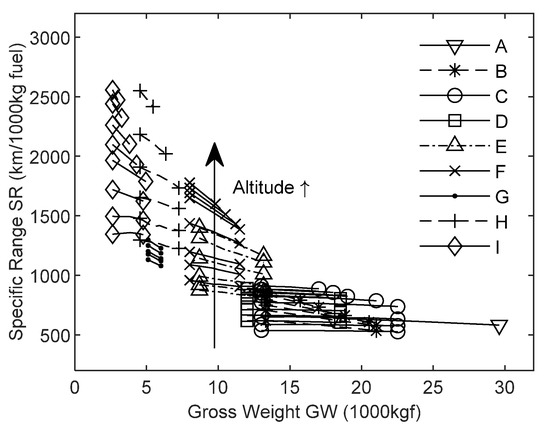
Figure 1.
Specific range data with altitude variation for the aircraft from the training set of Table 1.

Table 1.
Sets, samples, and aircraft weights.
2.2. Weights Breakdown and Weight of Fuel Burned
The total range Ra is divided into m steps (ΔRa = 1.852 km). The aircraft’s Gross Weight (GW) is assumed constant for the duration of one step and given by:
where OEW is the Operating Empty Weight. This weight includes the aircrew, all fluids necessary for operation, and the required operator items and equipment. In Equation (1), WP expresses the weight of the payload (including passengers), and WFi is the weight of usable fuel (by opposition to fuel trapped in the fuel system ducts, valves, and pumps), which is computed from the initial weight of usable fuel WF0 and the fuel burned during all preceding steps WFBi−1, so
The initial weight of usable fuel includes WFRes, the weight of fuel reserves. The fuel burned prior to reaching the cruise altitude (i.e., the sum of the start-up and maneuver fuel at the departure location, the take-off fuel, and the fuel to climb), is noted WFBS. Thus, the fuel burned during all preceding steps WFBi−1 is now given by
where WFBCj stands for the fuel consumed over the j-th range step in cruise conditions. It is calculated from the interpolated specific range SR(GW,Alt)-relationships (Figure 1):
For the preceding computations, the following hypotheses apply:
- The Weight of Fuel Reserves (WFRes) is taken as a fixed percentage of one of the aircraft’s representative masses, in the present case, the Maximum Take-Off Weight (MTOW). For civil airliners, a survey of the required reserves to satisfy the Airworthiness Authorities provisions (missed approach, hold, and diversion) among the training set led to a safe value of 3.5%. This value is less cautious than a flat 8% of the zero-fuel weight [7,25], but exceeds the 6% of the total fuel consumption taken as tolerance for reserves and trapped fuel [12].
- After a survey through the training set, the Weight of Fuel Burned at Start (WFBS) is estimated as 2% MTOW. This conservative value corresponds to the low-end of the 1.0% to 4.4% of the take-off gross weight found in [2,4,12,13,15,21].
- The gross weight is used for a linear interpolation of the specific range for different altitudes (6 samples), although better interpolation was obtained with a quadratic regression for 3 samples. In all cases, the goodness of fit R2 exceeded 0.99. The maximum relative errors computed after the interpolation process did not exceed 0.8%.
- Since the fuel that is required from the start of the descent to the arrival at the gate differs only by a small amount from the one that would be burned in cruise over the same distance, the missions end when flying atop the destination airfield, as in [17,25].
The step-wise computation of the total weight of fuel consumed for any range (Ra) and payload (WP) pair results in a matrix as illustrated in the top-right thumbnail in Figure 2. This matrix is then bracketed by the actual fuel and weight limitations to obtain the payload-range fuel-burned triplets shown in Figure 2. for an aircraft of the validation sample.
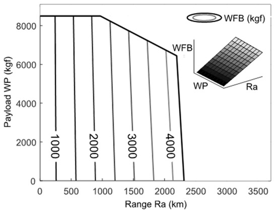
Figure 2.
Contours of the Weight of Fuel Burned (WFB) bracketed by the payload-range limitations for an aircraft from the training sample. The top-right thumbnail shows the unbracketed 3D fuel consumption surface.
2.3. Fuel Estimate Model Based on OEW
The Breguet range equation reads
after integration over the cruise segment. In Equation (5), the take-off weight TOW is given by TOW = OEW + WP + WFRes + WFB. Since the essence of the Breguet range equation is to model how fuel is consumed to fly a distance under the implications of the propulsion and aerodynamic parameters, and given that the gross weight has a significant impact onto this consumption, we proposed in [23] a knowledge-based response surface methodology involving solely the operating empty weight OEW. This polynomial response surface is now extended to lower OEW-values for civil turboprop-powered airliners. The response surface is based on the pair (Ra,WP) as independent variables
The p-coefficients are fitted to the actual data to yield the best R2-values. Given their potential influence on the end-result, we consider two hypotheses: cruise flight at constant altitude or cruise flight with stepwise increasing altitude. The constant altitude is taken as the maximum altitude at which the maximum gross weight can be sustained with a minimum rate of climb of 300 ft/min. For the changing altitude case, jumps vary between 20 hft to 50 hft depending on the aircraft type. In any case, the knowledge-based polynomial response surface comes with excellent correspondence with the original fuel consumption surface as the coefficients of determination (R2) are above 0.99.
As shown in Figure 3, the dominant terms of Equation (6) are the first order range term p10Ra and the independent term p00. As is apparent in Figure 4, the last is collocated with the weight of fuel burned at start (WFBS), as expected from the fixed percentage of the MTOW hypothesis.
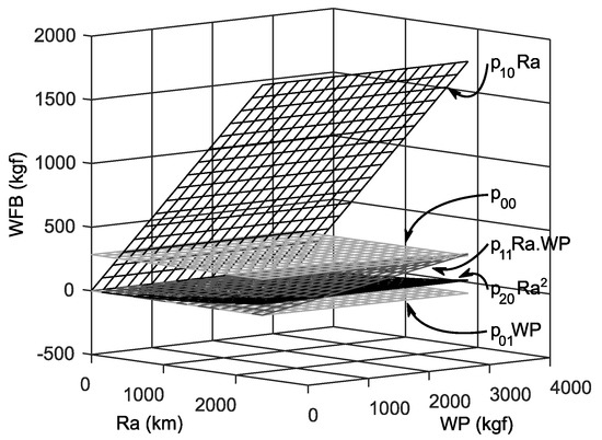
Figure 3.
Relative magnitude of the p-terms for an aircraft at constant altitude.
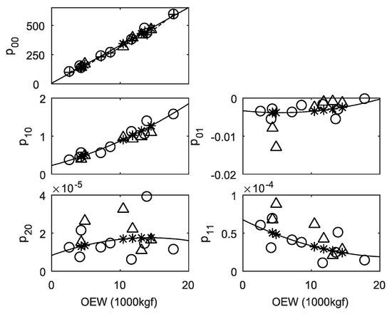
Figure 4.
p-Coefficients of the fuel consumption surface (WFB) fit for the maximum constant altitude case. ‘o’ training samples, ‘Δ’ validation samples, ‘*’ predicted value on the validation samples, on p00 ‘- - + - -’ Weight of Fuel Burned at Start WFBS = 2% of MTOW (Maximum Take-Off Weight).
In comparison with heavier military transports, the interaction term p11 and the range penalty term p20 have a more significant relative contribution but are only effective for long range and heavy missions. Since mission ranges do not exceed 2000–2500 km, the range penalty term p20 is not a significant contributor. That is another major difference with heavier transport aircraft. The payload represents an appreciable percentage of the operating empty weight, which typically does not exceed 39%–53% (see Table 1). These are comparatively lighter payloads than in the case of military transports. Consequently, the payload term p01 has only a very little influence.
Next, the model consists of expressing the response surface parameters (p-coefficients) in Equation (6) as:
The dependency on solely the operating empty weight is the key novel assumption. The underlying knowledgebase is that of similarity with the nearest in kind from an airframe and propulsion perspective. The strength behind the present method is that the operating empty weight is among the very first elements that are computed during the initial steps of the preliminary design process [4,12,13]. Equation (7) is shown in Figure 4 together with the original p-coefficients. The best fit for Equation (7) is detailed in Table 2. Excellent agreement is obtained on the dominant terms p00(OEW) and p10(OEW), as the respective coefficients of determination are above 0.99. For the independent term p00, the linear fit yields the percentage of the operating empty weight that closely matches the postulate on the weight of fuel burned at start WFBS (see Section 3). This suggests that this assumption could also be safely expressed in other terms as 3.2% of OEW. For p10(OEW), the agreement confirms the main assumption behind this method namely that given OEW and WP are present in the numerator and the denominator of the logarithm in Equation (5), then it is the fuel expressed as a percentage of OEW that is the leading term next to the range parameter. As the range parameter has little variation between near-in-kind designs and the consumed fuel depends directly on how much weight is carried, the OEW plays a preponderant role.
Table 2.
Response surface coefficients as a function of OEW (Operating Empty Weight):
Given their weak influence on Equation (6), the poor agreement on the other terms does not jeopardize the overall agreement of the model since the goodness of fit of the surface is modeled through Equations (6) and (7), and the original surface is above 0.93 for 11 samples and around 0.8 for the remaining 4.
The differences between preliminary design cycles with the Breguet range equation (Equation (5)) and the present OEW,q-model (Equations (6) and (7)) are summarized in Figure 5.
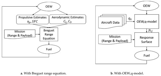
Figure 5.
Preliminary design cycles (a) with the Breguet range equation (Equation (5)) and (b) the OEW,q-model (Equations (6) and (7)).
3. Results, Validation of the OEW,q-Model, and Discussion
3.1. Instantaneous Fuel Consumption Figure of Merits
The database allows us to analyze common figures of merit such as Fuel Flow Rates, Specific Range, and Specific Fuel Consumption. When looking at the fuel flow rates FF (comprising all engines) in the maximum cruising constant altitude assumption shown in Figure 6, we establish a linear relationship
with a goodness of fit of 0.83, but the mean relative error obtained with this approach is of the order of 14%. This trend is higher than the trend established in [23] where the set consists primarily of larger, more powerful engines, which are known comparatively to consume less [5].
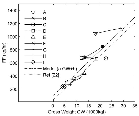
Figure 6.
Hourly fuel flow and gross weight dependence at constant altitude.
Based on the data from Figure 7, the specific range is expressed as a power-fit applied to the gross weight as given in Table 3 together with R2. The model is built either on the hypothesis of a constant altitude flight at the maximum cruise altitude (see Section 2.3), or for the minimum cruising altitude found in the flight manuals. The coefficients are given in Table 3 together with the R2-values. Given the goodness of fit, this model should be used with care since the mean relative error for both hypotheses is of the order of 10% with actual values ranging between 0.4% and 36.1%. The largest errors occur typically for aircraft lighter than 12,500 kgf. Next to confirming the trend set for the light military transport category in [23], the present data confirm the strong dependency of specific range to gross weight and altitude and, thereby, invalidate the assumption of a constant value.
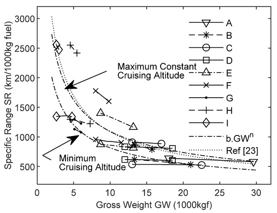
Figure 7.
Specific range variation with the gross weight for the maximum constant cruise altitude, and for the minimum cruise altitude. See Table 3 for model coefficients.
Table 3.
Specific range (km/1000kg fuel) power-fit to gross weight (kgf) at the maximum constant altitude, and at the minimum cruise altitude:
We also plotted the power Specific Fuel Consumption SFC depending on the gross weight in Figure 8, since this approach is often used in conjunction with the Breguet range equation. Reported values from the literature range from 0.23–0.37 kg/kW/hr as shown in Figure 8. Current data return a mean SFC of 0.362 kg/kW/hr and a median of 0.361 kg/kW/hr, which are close to the maximum bounds found in the literature [1,6,9,12,13,15,17,26]. Figure 8 indicates that for aircraft in the present weight range, the one standard deviation interval 0.3–0.42 kg/kW/hr is better suited. Although the samples in [23] all featured a strong dependence of the Specific Fuel Consumption upon the gross weight, some samples in Figure 8 do not. This confirms the reservations made in [21,22,23,27] about the widely accepted assumption consisting of using a constant Specific Fuel Consumption along the integration of the Breguet range equation.
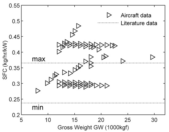
Figure 8.
Power Specific Fuel Consumption in cruise at maximum constant altitude.
3.2. WFB-Predictions and Validation of the OEW,q-Model
Once an operating empty weight is given, the OEW,q-model allows us to predict the response surface coefficients through Equation (7) and in Table 2. Then the weight of fuel burned can be computed for any mission. The accuracy of the model is shown in Figure 9 for an aircraft of the validation sample. For the overall training samples, the mean error on the prediction of the weight of fuel burned versus the actual weight of fuel consumed does not reach 2% of the operating empty weight. This error never exceeds 4% for the validation samples. The highest errors occur systematically for the region of the payload-range diagram that corresponds to the maximum fuel line (as in Figure 9). In comparison, the mean error when working with the Breguet range equation () on the validation set is of 3% OEW, but the maximum error reaches 10%. This behavior is shown in Figure 10 for the same sample as in Figure 8.
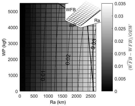
Figure 9.
Relative error on the fuel consumption between the model estimate and the actual value WFB in the maximum constant altitude assumption for a validation sample. The thumbnail shows the actual unbracketed WFB surface in grey tones and the estimate -surface in shade.
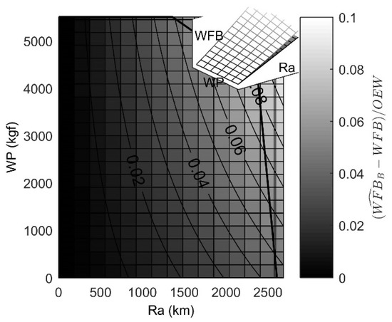
Figure 10.
Relative error on the fuel consumption between the estimate with the Breguet range equation (Equation (5)) on the same case as in Figure 9. The thumbnail shows the actual unbracketed WFB surface in gray tones and the Breguet estimate -surface in shade.
Next to the analysis of the individual p-coefficients in Section 2.3 and Figure 4, the accuracy shown in Figure 9 with the OEW,q-model confirms the correctness of the principal assumption behind the model, i.e., that the fuel consumed over a distance is mainly driven by the operating empty weight.
3.3. Influence of Altitude on the OEW,q-Model
The coefficients from Table 2 are also given for the stepwise increasing altitude hypothesis, in which the flight altitude is increased concurrently as the current gross weight decreases. By doing so, the range can be further maximized. As was the case with the military transports, the change of hypothesis has no significant impact on the accuracy of the model as is illustrated in Figure 11 for a sample from the validation set. The mean error on the predicted fuel consumed does not exceed 3% of the operating empty weight for the whole validation set. As shown on Figure 12, the model offers significantly better accuracy than the Breguet range equation when applied to stepwise increasing altitudes.
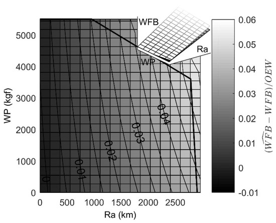
Figure 11.
Relative error on the fuel consumed (WFB) between the predicted value and the actual value for the increasing altitude case on a validation sample. The thumbnail shows the actual unbracketed fuel consumption matrix in gray tones and the predicted -matrix in shade.
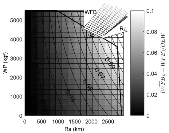
Figure 12.
Relative error on the fuel consumed (WFB) between the estimate with the Breguet range equation (Equation (5)) on the same case as in Figure 11. The thumbnail shows the actual unbracketed fuel consumption matrix in gray tones and the Breguet estimate -matrix in shade.
3.4. Influence of Temperature on the OEW,q-Model
Since increasing the exterior temperature is known to have a negative impact on the performance of the propulsion system, the influence of a +10° deviation from cruise ISA-conditions has been assessed. The fuel flow typically increases by +2% to +7% so that the specific range is decreased for identical cruise speeds. On top of that, weight or altitude limitations could raise from higher exterior temperature, though this is out of the scope of the present method.
4. Conclusions
It is shown that the response surface describing the weight of fuel burned for every possible payload-range combination is largely determined by the first order range term (p10 Ra) in Equation (6). A strong correlation has been found between the range term and the operating empty weight. In other words, while fuel is burned to displace an aircraft’s gross weight over a certain range, it is essentially the aircraft’s operating empty weight that determines the total fuel consumption, while the payload or the deadweight fuel carried over long flights play, herein, only a minor role. Long missions (i.e., above 2000 km) come with a fuel penalty for carrying deadweight fuel over the first legs. Therefore, the OEW,q-model is proposed to make an early and reliable estimate of the mission fuel weight any range and payload pairs. The rationale behind the OEW,q-model is that comparable aircraft designs can effectively be identified through their operating empty weight within the present range of efficiency of the propulsion. It is based on actual aircraft data.
The proposed OEW,q-model is applicable to turboprop-powered civil airliners and transports since aircraft developed for military duties were dealt with in [23]. Civil and military types differ strongly in the OEW-range that is considered. Although the methodology is identical, it is not straightforward to use the response surface coefficients found on one data set for the other given the marked differences in operating empty weight. These differences come from distinct operational requirements that led to separate design solutions in terms of structure and propulsion. Because of its accuracy, which is lower than 4% of the operating empty weight, and given its dependence solely on the operating empty weight to educe a response surface, the model is particularly suited for the conceptual or preliminary design stages, or for benchmarking. Because of its accuracy and the low number of input parameters (only the OEW is required next to the present coefficients), it outperforms models, such as the Breguet range equation, which are available in the wide body of literature dedicated to aircraft design.
Additionally, empirical correlations are also established for the fuel flow rate and the specific range as functions of an aircraft’s gross weight. Moreover, it is shown that the amount of fuel consumed from the engine start to the end of the climb can be safely expressed as 3.2% of OEW instead of a fixed percentage of the maximum take-off weight.
Author Contributions
Conceptualization, B.G.M. and A.H.; methodology, B.G.M. and A.H.; software, A.H.; validation, B.G.M. and A.H.; formal analysis, B.G.M. and A.H.; investigation, A.H.; resources, A.H.; data curation, A.H.; writing—original draft, B.G.M. All authors have read and agreed to the published version of the manuscript.
Funding
This research received no external funding.
Conflicts of Interest
The authors declare no conflict of interest.
Nomenclature
| a,b | Regression coefficients |
| Alt | Altitude |
| D | Drag (N) |
| FF | Fuel Flow rate (kg/hr) |
| g | Gravitational acceleration (m/s2) |
| GW | Gross Weight |
| L | Lift (N) |
| MTOW | Maximum Take-Off Weight (kgf) |
| n | Regression exponent |
| OEW | Operating Empty Weight (kgf) |
| p,q | Polynomial coefficients |
| Ra | Range (km) |
| SFC | Power specific fuel consumption (kg/kW/hr) |
| SR | Specific Range (km/1000kg of fuel) |
| TOW | Take-Off Weight (kgf) |
| WF | Weight of Fuel (kgf) |
| WFB | Weight of Fuel Burned (kgf) |
| WFBC | Weight of Fuel Burned for Cruise (kgf) |
| WFBS | Weight of Fuel Burned for Starting (kgf) |
| WFRes | Weight of Fuel Reserves (kgf) |
| ZFW | Zero Fuel Weight (kgf) |
| Propeller propulsive efficiency | |
| Predicted value | |
| Breguet estimate | |
| Note: Altitudes are expressed in hectofeet (hft) according to common aeronautical practice. | |
| Note: Kilogram-force units (kgf) are used for weights that are otherwise expressed in mass units in standard aeronautical practice. | |
References
- Babikian, R.; Lukachko, S.; Waitz, I. The historical fuel efficiency characteristics of regional aircraft from technological, operational, and cost perspectives. J. Air Transp. Manag. 2002, 8, 389–400. [Google Scholar] [CrossRef]
- Corke, T.C. Design of Aircraft; Prentice Hall: Upper Saddle River, NJ, USA, 2003. [Google Scholar]
- Filippone, A. Data and performances of selected aircraft and rotorcraft. Prog. Aerosp. Sci. 2000, 36, 629–654. [Google Scholar] [CrossRef]
- Howe, D. Aircraft Conceptual Design Synthesis; Professional Engineering Publishing: London, UK, 2000. [Google Scholar]
- Ibrahim, K. Selecting principal parameters of baseline design configuration for twin turboprop transport aircraft. In Proceedings of the 22nd Applied Aerodynamics Conference and Exhibit, Providence, RI, USA, 16–19 August 2004. Number AIAA 2004–5069. [Google Scholar] [CrossRef]
- Kundu, A.K. Aircraft Design; Cambridge University Press: Cambridge, UK, 2010. [Google Scholar]
- Lee, H.-T.; Chatterji, G.B. Closed-form takeoff weight estimation model for air transportation simulation. In Proceedings of the 10th AIAA Aviation Technology, Integration and Operations Conference, Ft. Worth, TX, USA, 13–15 September 2010; Volume 2. [Google Scholar] [CrossRef]
- Liem, R.P.; Mader, C.A.; Martins, J.R. Surrogate models and mixtures of experts in aerodynamic performance prediction for aircraft mission analysis. Aerosp. Sci. Technol. 2015, 43, 126–151. [Google Scholar] [CrossRef]
- Marinus, B.G.; Poppe, J. Data and design models for military turbo-propeller aircraft. Aerosp. Sci. Technol. 2015, 41, 63–80. [Google Scholar] [CrossRef]
- Nightingale, W.I.M. Aeroplane weight analysis. Aircr. Eng. Aerosp. Technol. 1945, 17, 250–253. [Google Scholar] [CrossRef]
- Obert, E.; Slingerland, R. Aerodynamic Design of Transport Aircraft; IOS Press BV: Amsterdam, The Netherlands, 2009. [Google Scholar]
- Raymer, D.P. Aircraft Design: A Conceptual Approach; AIAA: Reston, VA, USA, 2006. [Google Scholar] [CrossRef]
- Roskam, J. Part 1: Preliminary sizing of airplanes. In Airplane Design; DARcorporation: Lawrence, KS, USA, 2002; ISBN 9781884885556. [Google Scholar]
- Roskam, J.; Lan, C.-T.E. Airplane Aerodynamics and Performance; DARcorporation: Lawrence, KS, USA, 1997. [Google Scholar]
- Schaufele, R.D. The Elements of Aircraft Preliminary Design; Aries Publications: Santa Ana, CA, USA, 2000. [Google Scholar]
- Stinton, D. The Design of the Airplane; BSP Professional Books: Oxford, UK, 1983. [Google Scholar]
- Torenbeek, E. Synthesis of Subsonic Airplane Design; Delft University Press-Kluwer Academic Publishers: Delft, The Netherlands, 1982. [Google Scholar]
- Torenbeek, E. Prediction of wing group weight for preliminary design. Aircr. Eng. Aerosp. Technol. 1971, 43, 16–21. [Google Scholar] [CrossRef]
- Vouvakos, X.; Kallinderis, Y.; Menounou, P. Preliminary design correlations for twin civil turboprops and comparison with jet aircraft. Aircr. Eng. Aerosp. Technol. 2010, 82, 126–133. [Google Scholar] [CrossRef]
- Breguet, L. Calcul du poids de combustible consommé par un avion en vol ascendant. In Comptes Rendus Hebdomadaires des Séances de l’Académie des Sciences; Académie des Sciences: Paris, France, 1923; pp. 870–872. [Google Scholar]
- Randle, W.E.; Hall, C.A.; Vera-Morales, M. Improved range equation based on aircraft flight data. J. Aircr. 2011, 48, 1291–1298. [Google Scholar] [CrossRef]
- Torenbeek, E. Cruise performance and range prediction reconsidered. Prog. Aerosp. Sci. 1997, 33, 285–321. [Google Scholar] [CrossRef]
- Marinus, B.G.; Maison, J. Fuel weight estimates of military turbo-propeller transport aircraft. Aerosp. Sci. Technol. 2016, 55, 458–464. [Google Scholar] [CrossRef]
- BADA v3.13. Base of Aircraft Data, March 10 2017. Available online: www.eurocontrol.int/services/bada (accessed on 15 May 2017).
- Kroo, I. Aircraft Design: Synthesis and Analysis; Desktop Aeronautics, Inc.: Stanford, CA, USA, 2001. [Google Scholar]
- Fielding, J.P. Introduction to Aircraft Design; Cambridge University Press: Cambridge, UK, 1999. [Google Scholar] [CrossRef]
- Cavcar, A.; Cavcar, M. Approximate solutions of range for constant altitude-constant high subsonic speed flight of transport aircraft. Aerosp. Sci. Technol. 2004, 8, 557–567. [Google Scholar] [CrossRef]
© 2020 by the authors. Licensee MDPI, Basel, Switzerland. This article is an open access article distributed under the terms and conditions of the Creative Commons Attribution (CC BY) license (http://creativecommons.org/licenses/by/4.0/).