Impact Evaluation of Grid-Connected PV Systems on PQ Parameters by Comparative Analysis based on Inferential Statistics

Abstract

The intermittent injection of power and the nature of power electronic devices used for photovoltaic (PV) systems can affect the power quality (PQ) of the grid to which they are connected. This study proposes to quantify and evaluate the impact of PV injection on the PQ of a low-voltage (LV) network by applying a statistical analysis through hypothesis testing for the mean comparison of populations of parameters with and without a PV system. The effects of PV power injection and load demand at the point of common coupling on PQ are monitored. The methodology includes the selection and monitoring of PQ, the use of a matrix for classification of data with similar load and PV power injection conditions, and the application of the Wilcoxon rank sum test. This methodology was applied to evaluate the impact of a 9.8 kWp PV system on the PQ of an LV network.

1. Introduction

In 2018, the installed photovoltaic (PV) capacity reached 505 GW worldwide. The impact of PV systems in power systems can be positive or negative depending on their size and location, and features of the electrical network. Some positive impacts can be reduction of power loss, improvement of voltage profile, and intensive use of transmission lines [1,2,3,4,5,6]. However, the intermittent power injection and the operating characteristics of inverters used in PV systems may cause a negative impact on a network, such as protection coordination failures, high losses in conductors, voltage fluctuations, harmonic distortion, and grid-side disturbances [5,6,7,8].

In recent years, researchers have studied the impact of integrated PV systems by monitoring or modelling and the simulation of electrical behaviour at the point of common coupling (PCC). The majority of these studies analyse power quality (PQ) parameters such as Vrms, power factor (PF), total harmonic distortion of current/voltage (THDI/THDV), individual harmonic distortion of current/voltage (IHDI/IHDV), short-term/long-term perceptibility (Pst/Plt), and voltage imbalance (V₂/V₁).

Table 1. Studies related to impact of photovoltaic (PV) systems on power quality (PQ) parameters.

Reference	Duration	Parameters	Simulation	Measurement
[9] (2012)	-	THDI, THDV, IHDV, IHDI	√	√
[10] (2013)	-	PF, Vrms, IHDI, THDI	√	-
[11] (2013)	2 years	THDI, IHDI, PST, Voltage variations	√	-
[12] (2013)	1 day	THDI, IHDI	√	√
[13] (2015)	1 week	THDI, THDV, PF	√	√
[14] (2016)	2 years	THDV, THDI, IHDV, IHDI	-	√
[15] (2016)	-	IHDV, IHDI, THDV, THDI	√	-
[16] (2016)	3 months	Vrms, THDV	-	√
[17] (2017)	2 days	THDI, THDV, Vrms	-	√
[18] (2018)	1 week	THDI, IHDV	-	√
[19] (2018)	-	THDV, THDI, IHDV, IHDI	-	√
[20] (2018)	7 months	PST, PLT, THDV, THDI, PF, V2/V1	-	√
[21] (2019)	7 weeks	THDI, THDV, IHDI, IHDV, pf, Vrms, Pst, Plt	-	√

lists some of these studies; several of them include THD/IHD analysis through on-site measurements during several time periods.

PV system integration in low-voltage (LV) and medium-voltage (MV) networks can increase the Vrms and decrease the THDV at the PCC [9,10,11,16,17,18,19,21]; this effect seems to be more noticeable for higher PV power injections.

Urbanetz et al. [9] studied the impact of a 12 kWp PV plant in an urban environment and found a slight reduction in THDV from 1.98% to 1.83% at the PPC; likewise, they observed increases in the effective voltage according to the connected load and the distance between the PCC and the electrical substation.

Pinto et al. [16] presented results of a PQ analysis for a PV system connected to an LV rural network; the voltage at the PCC increased and remained very close to the allowable limit. Similarly, Grycan et al. [18] reported that an increase in the PV power injection from a solar farm caused an increase in Vrms at the PCC and a decrease in voltage distortion.

Moreover, some research has shown that the THDI and IHDI are significant for a low PV power injection but decrease with a higher PV power injection [10,11,12,13,14,15,17,18,19,20]. Nemes et al. [14] studied the effect of a 3 kWp PV system in an LV network from the comparison of PQ parameters of a grid using the limits of the IEEE 519, IEC 61000, and EN 50160 standards. Ortega et al. [11] monitored and evaluated PQ parameters in an 800 kWp plant and showed that an injection of PV power higher than 90% of the installed capacity reduced the THDV and a low PV power injection caused distortions and current imbalance exceeding the allowable limits.

Leite et al. [19] presented an experimental analysis of the distortion of current and voltage before and after the installation of a 3.38 kWp PV system in an LV network based on the IEEE 519 standard. Similarly, Granja et al. [20] conducted a PQ analysis at the PCC between a 7.8 kWp PV system and an LV network. The results showed that the PV system had no negative impact on either the steady-state voltage or the power factor, and no overvoltages occurred. Furthermore, no undervoltages or violations for THDV were observed; however, the total demand distortion (TDD) maximum values were above the established limit with PV power injection.

These studies can be tackled by different approaches. Some authors compared specific PQ parameters with limits or ranges established by standards [10,11,14,18]; other authors classified the data and compared them according to PV injection levels [13,19]; and some other authors compared the parameters for scenarios with and without injection to find the average, maximum, or minimum values [9,15,16,17,20].

Based on a review of studies, the study of the impact of PV power injection has been approached mainly through on-site measurements by applying a comparative deterministic analysis of PQ parameters; so, performing studies that consider PQ parameters as random variables and introduce statistical analysis of data can strengthen the quality of findings.

Therefore, this study present a methodology based on a statistical comparative analysis of the variation of thirteen PQ parameters in a LV network. The measurements of the selected twelve single-phase PQ parameters (Vrms, TDD, THDV, THDI, IHDV₃, IHDV₅, IHDV₇, IHDI₃, IHDI₅, IHDI₇, power factor, and Pst) and one three-phase PQ parameter (V₂/V₁).

It is considered that the impact of PV power injection on PQ depends on both the injected PV power and the load demand at the PCC. Thus, a scenario matrix was created that grouped data into scenarios according to load and PV power injection ranges. Likewise, the collected data during periods without a PV system were grouped in scenarios according only to load range.

Subsequently, the amount of data and average values were determined per scenario (sample population). Then, a statistical analysis was applied through hypothesis testing for mean comparison of populations of parameters with and without PV systems to determine whether the PV system impacts on PQ parameters at the PCC. The compared populations were scenarios with and without PV injection within the same load range. The variations of the PQ parameters were analysed through the non-parametric Wilcoxon rank sum test because the data in the scenarios were not normally distributed.

The methodology was used to analyse the effect of the power injection of a 9.8 kWp PV system in a LV electrical network at a university building in Bucaramanga, Colombia.

2. Methodology

The proposed methodology by authors [20] consists of five steps: description of the PV system; selection of the PQ parameters; description of the monitoring system; classification of the data; and comparison of the means between two sample populations, the first with PV power injection and the second without PV power injection, using an inferential statistics test. Figure 1 shows a schematic diagram of the methodology.

2.1. Case Study

The PV system shown in Figure 2 was installed at the Edificio de Ingenieria Electrica (EIE) of the Universidad Industrial de Santander (UIS). This university is located at 960 masl, 7.13° North and 73.13° West in Bucaramanga, Colombia. The average ambient temperature is 24 °C during the day, and 27 °C between 6 a.m. and 6 p.m. (daylight hours). The average solar irradiance is 4.9 kWh/m²/day, which varies between 2.0 kWh/m²/day and 7.6 kWh/m²/day. The wind speed in the UIS campus varies between 1.0 and 1.5 m/s [22].

This PV system has a capacity of 9.8 kW and is formed by 37 PV panels (255–270 W) and 37 Enphase M250 microinverters. Each transformerless microinverter manages one PV panel and injects the generated power to network through two-phase connection. These microinverters are connected in Δ connection to a distribution board on the fourth floor of the building.

2.2. Selection of Power Quality (PQ) Parameters and Evaluation Criteria

In total, thirteen parameters were studied. Twelve of them were applied per phase: Vrms, Pst, TDD THDV, THDI, IHDI (3rd, 5th, and 9th), IHDV (3rd, 5th, and 7th), and power factor; while the voltage imbalance was analysed as a three-phase parameter.

Table 2. Reference values for PQ parameters.

PQ Parameter	Reference Value
Vrms	0.90 ≤ Vnompu ≤ 1.10
Pst	≤ 1.0
THDV	≤ 8%
IHDV (3rd, 5th, and 7th)	≤ 5%
THDI	-
IHDI (3rd, 5th, and 7th)	Table 2 IEEE Standard 519 of 2014
TDD
Power factor	≥ 0.9
V2/V1	0.5–2.0%

shows the ranges of variation and limits of the selected parameters, which were obtained from revision of the standards IEC 61000-4-30, IEC 61000-4-15, IEEE 1159: 2009, and IEEE 519: 2014, and the Colombian PQ framework formed by CREG resolutions (070 of 1998, 024 of 2005, 016 of 2007, and 065 of 2012).

According to the requirements for studies of PQ of IEC 61000-4-30, IEEE 519, Annex B of IEC 61000-4-30, and Colombian regulations, the measuring equipment selected is Class A (PQube3 Analyzer and Acuvim IIR) with 10-min data aggregation intervals during time interval measurement, which must be at least a week.

2.3. Equipment

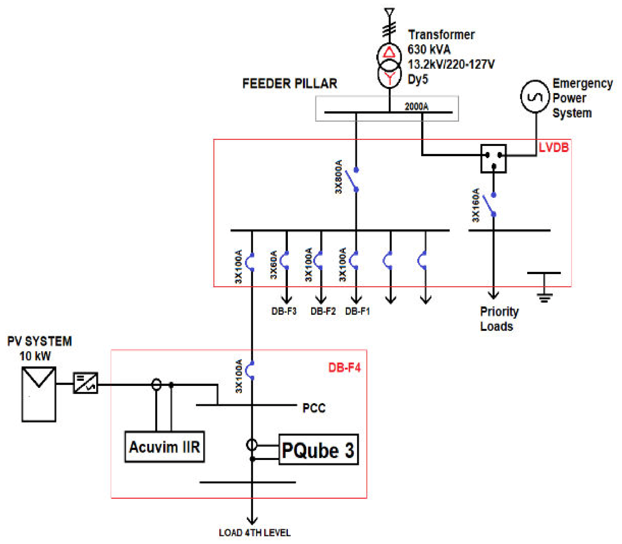
Figure 3 shows the single-line diagram of the electrical network of the EIE building, which allows to see the location of the PCC, connection of the PV system, and the two Class 0.2 smart meters. A PQube 3 analyser was used to monitor the power supply connection at the fourth floor; this meter was configured with a sampling frequency of 30.72 kHz (512 samples per cycle). An Acuvim IIR analyser was used to monitor the PV power injection at the PCC and recorded the effective voltage and current, active power, reactive power, apparent power, THDV, THDI, IHDV, IHDI, and voltage imbalance.

2.4. Data Classification into Scenario Matrix

The behaviour of parameters at the PCC may depending on the PV power and the power demand; therefore, it is necessary to establish a strategy, like a matrix, to classify the data into scenarios according to the ranges of these two variables. Thus, a scenario matrix is a tool to analyse data obtained for different instants with similar PV power and power demand conditions. In a manner slightly similar to this proposal, some studies evaluate the indicators, taking into account the level of PV injection [13,19]; other studies compare of parameters during PV injection with standards [10,11,14,18] or compared average, maximum, or minimum values of indices for two conditions: with and without PV injection [9,15,16,17,20]. The scenario matrix was created as follows:

(1)

Define the base values of PV power and load power considering the maximum values recorded for these two variables by phase.

(2)

Determine the number of intervals of PV power (m) and the load power (n) in order to group the logged data for each phase. Each cell of the matrix (PV power interval i, load power interval j) corresponds to a scenario. Initially, m = 10 and n = 10, so the matrix allowed the classification of data into 100 scenarios or vectors when PV power was injected. In this study, the group of data for n = 1 was divided in two intervals because of amount of data; therefore, n = 11 and the total scenarios or vectors is 110.

(3)

Create $Nk$ mxn matrices, where $Nk=3·N{k}_{1\phi }+N{k}_{3\phi }$, $N{k}_{1\phi }$ is the number of single-phase PQ parameters to be analysed (12 per phase), and $N{k}_{3\phi }$ is the number of three-phase PQ parameters (V₂/V₁). In total, this study analysed 37 matrices.

(4)

Aggregate an external column to the matrix for classifying data obtained for without PV power injection condition. Due to this column is formed by n scenarios, the size of the matrix is 11 x 11.

(5)

Record the data and classify them into the matrix corresponding to each parameter. The total number of vectors or scenarios (NV) was equal to n(m + 1)Nk; that is, 4.356 single-phase vectors and 121 three-phase vectors, in total 4.477 scenarios.

Figure 4 shows the scenario matrix. The power demand and PV injection intervals are located on the left and top, respectively. The cyan values correspond to the interval bounds in kVA for Phase A.

From the maximum load (2.18 kVA) and maximum PV power (3.07 kVA) in Phase A, the base values of load (2.2 kVA) and PV power (3.1 kVA) were selected. Then, 10 PV power injection intervals to classify data were determined: 0–0.31, 0.31–0.62, 0.62–0.93, 0.93–1.24, 1.24–1.55, 1.55–1.86, 1.86-2.17, 2.17–2.48, 2.48–2.79, and 2.79–3.10 in kVA. Eleven load intervals were defined as 0–0.055, 0.055–0.22, 0.22–0.44, 0.44–0.66, 0.66–0.88, 0.88–1.10, 1.10–1.32, 1.32–1.54, 1.54–1.76, 1.76–1.98, and 1.98–2.20 in kVA.

2.5. Inferential Statistical Test

Hypothesis testing is a tool to determine if the means of two sample populations are equals. In this study, the means of the two scenarios were compared, with PV injection (${\overline{x}}_{PVSOn\left(i,j\right)}$) and without PV injection (${\overline{x}}_{PVSOff\left(i\right)}$), for intervals $i$ and $j$. The statement of this comparison were proposed:

$$H_0:{\overline{x}}_{PVSOn\left(i,j\right)}={\overline{x}}_{PVSOff\left(i\right)}$$

(1)

$$H_1:{\overline{x}}_{PVSOn\left(i,j\right)}\ne {\overline{x}}_{PVSOff\left(i\right)},$$

(2)

where H₀ and H₁ are the null and alternative hypothesis, respectively. This test was a two-tailed test with a typical α confidence interval of α = 0.05.

H₀ acceptance occurred when the P value of the test was greater than α; otherwise H₀ was rejected. The acceptance of H₀ means there was no statistical difference between the two means; therefore, it was assumed that the PV power injection did not affect the parameter. However, the rejection of $H_0$ indicates the PV power injection affected the parameter.

In order to define the type of test (parametric or non-parametric) that must be used, a normality test was applied to data from each scenario, like the Kolgomorov–Smirnov (K–S) test with a confidence level of 95%. The results showed insufficient evidence to accept the assumption of normality of data from every scenario, which is in line with results obtained by Sancho et al. [23], who applied the K–S test on the data relating to THDV and other harmonics and concluded that data sets of the harmonics studied are normally distributed. For this reason, the non-parametric Wilcoxon rank sum test was chosen to allow the analysis of two independent sample populations of sizes n₁ and n₂ [24].

3. Analysis of Results

The monitoring time was approximately seven weeks, 32 days with PV power injection, and 14 days without PV power. Because of the PV system injected power only during sun-hour time, data were taken between 6:10 a.m. and 6:00 p.m. of each day. The measurement effectiveness was of 99.064% (3281 measurements) with respect to the potential monitoring (3312 measurements); this means the lost records of data during the download were 0.936% (31 measurements). Therefore, each scenario matrix allowed classifying 3281 data in 121 intervals for each parameter.

3.1. Point of Common Coupling (PCC) Characterization

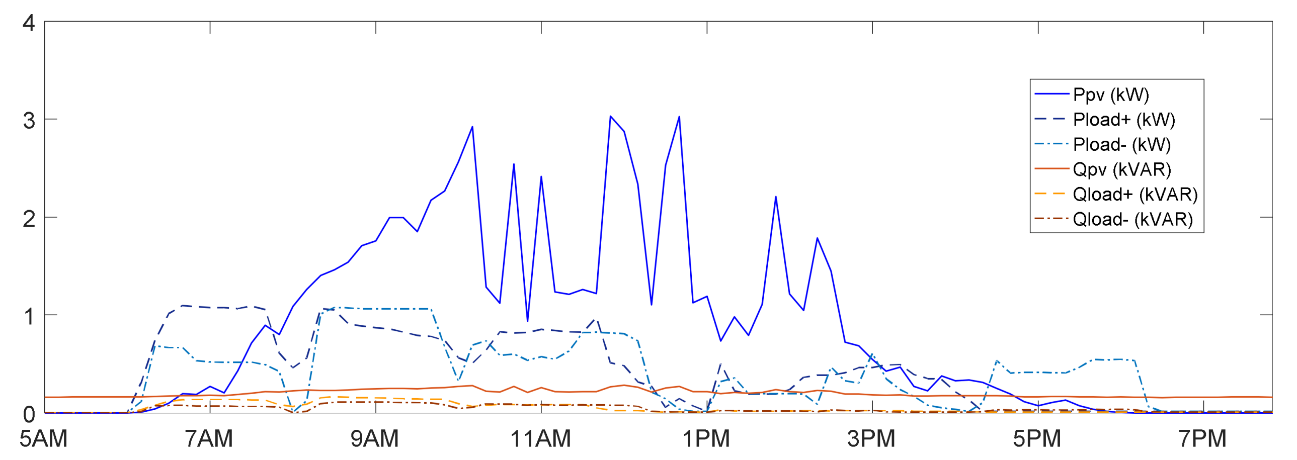
As expected, the behaviour of power injected by the PV system at the PCC were similar for three phases. The active power described the high variation of the solar irradiance and reached maximum values of 3 kW per phase; while the reactive power varied slightly and its value remained near 180 VAR per phase for all time. Significant differences between the curves of active and reactive power for the days with injection (P_load+ and Q_load+) and without injection (P_load- and Q_load-) are shown in Figure 5, Figure 6 and Figure 7.

Figure 8 shows that the Vrms and THDV at the PCC during a week for each phase; both decreased between 7:00 a.m. and 4:00 p.m. from Monday to Saturday. The THDV reached its highest value (4%) on Sunday because of the low load. These behaviours can be seen by comparing Figure 8 and Figure 9, where the latter corresponds to the apparent power demand in kVA.

Figure 10 shows the TDD variation during the periods with the highest power consumption; however, not all the peaks of this indicator coincided with those of the power peaks.

3.2. Probability of Occurrence of Each Scenario

A scenario matrix allows knowing the frequency of occurrence of each scenario, which helps to determine the intensity of the possible affectation of a particular scenario. In addition, it shows the average value of each parameter for each scenario. The creation of the matrix for Phase A is described next.

A measurement corresponds to a dataset that was logged at the same instant or lapse (by phase) and is associated with a scenario. Each scenario was defined by the apparent load power and the apparent power from the PV system during that lapse. The simultaneous measurements for the three phases may not correspond to the same scenario because most of the loads in the building were single-phase loads.

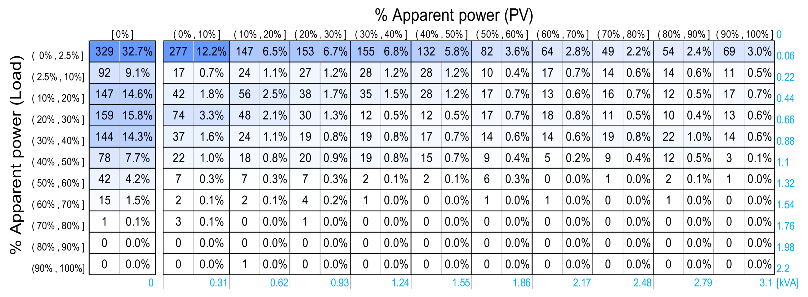
In total, 3281 measurements were taken, each one with 37 data, 12 data per phase, and one three-phase data. Each data was a PQ parameter and was classified into the matrix for that parameter. Each matrix allowed the classification of 2274 data with PV injection in the $PVS On\left(i,j\right)$ scenarios and 1007 data without PV injection in the $PVS Off\left(i\right)$ scenarios. Figure 11, Figure 12 and Figure 13 show the frequency matrix of each scenario for each phase.

The frequency matrix shows that the $PVS Off\left(4\right)$ scenario with a load range of (30%–40%] had probabilities of occurrence of 14.3% (144 data), 10.1% (102 data), and 7.0% (70 data) for phases A, B, and C, respectively. The $PVS On\left(I=5,j\right)$ scenarios had probabilities of occurrence of 8.6% (Phase A), 5.5% (Phase B), and 3.5% (Phase C).

Table 3. Probability of occurrence of scenarios with load ranges of 0%–30% and 30%–100%.

	Load	Phase A	Phase B	Phase C
PVS On	(0%–30%]	82.8%	88.8%	85.9%
	(30%–100%]	17.2%	11.2%	14.1%
PVS Off	(0%–30%]	72.2%	82.0%	78.9%
	(30%–100%]	27.8%	18.0%	21.1%

shows that the PVS On and PVS Off scenarios in the 0%–30% range had an approximately 70-90% probability of occurrence for each phase.

Table 4. Scenarios of greater probability for each phase.

Phase	Without PV Injection				With PV Injection
	Scenario	Load	PO		Scenario	Load	PV Injection	PO
A	I = 1	(0–2.5%] 0–0.06 kVA	32.7%		I = 1; j = 1	(0–2.5%] 0–0.06 kVA	(0–10%] 0–0.31 kVA	12.2%
	i = 4	(20–30%] 0.440–66 kVA	15.8%		i = 1; j = 4	(0–2.5%] 0–0.06 kVA	(30–40%] 0.93–1.24 kVA	6.8%
	i = 3	(10–20%] 0.22–0.44 kVA	14.6%		i = 1; j = 3	(0–2.5%] 0–0.06 kVA	(20–30%] 0.62–0.93 kVA	6.7%
B	i = 2	(2.5–10%] 0.05–0.18 kVA	61.4%		i = 2; j = 1	(2.5–10%] 0.05–0.18 kVA	(0–10%] 0–0.31kVA	16.9%
	i = 4	(20–30%] 0.36–0.54 kVA	12.1%		i = 2; j = 4	(2.5–10%] 0.05–0.18 kVA	(30–40%] 0.93–1.24 kVA	9.6%
	i = 5	(30–40%] 0.54–0.72 kVA	10.1%		i = 2; j = 3	(2.5–10%] 0.54–0.72 kVA	(20–30%] 0.62–0.93 kVA	9.2%
C	i = 1	(0–2.5%] 0–0.04 kVA	44.7%		i = 1; j = 1	(0–2.5%] 0–0.04 kVA	(0–10%] 0–0.31 kVA	13.4%
	i = 4	(20–30%] 0.32–0.48 kVA	14.3%		i = 1; j = 2	(0–2.5%] 0–0.04 kVA	(10–20%] 0.31–0.62 kVA	7.4%
	i = 2	(2.5–10%] 0.04–0.16 kVA	13.9%		i = 1; j = 4	(0–2.5%] 0–0.04 kVA	(30–40%] 0.93–1.24 kVA	7.1%

presents the three scenarios with the highest occurrences by phase, which occurs for low load and low PV injection conditions.

3.3. Wilcoxon Rank Sum Test

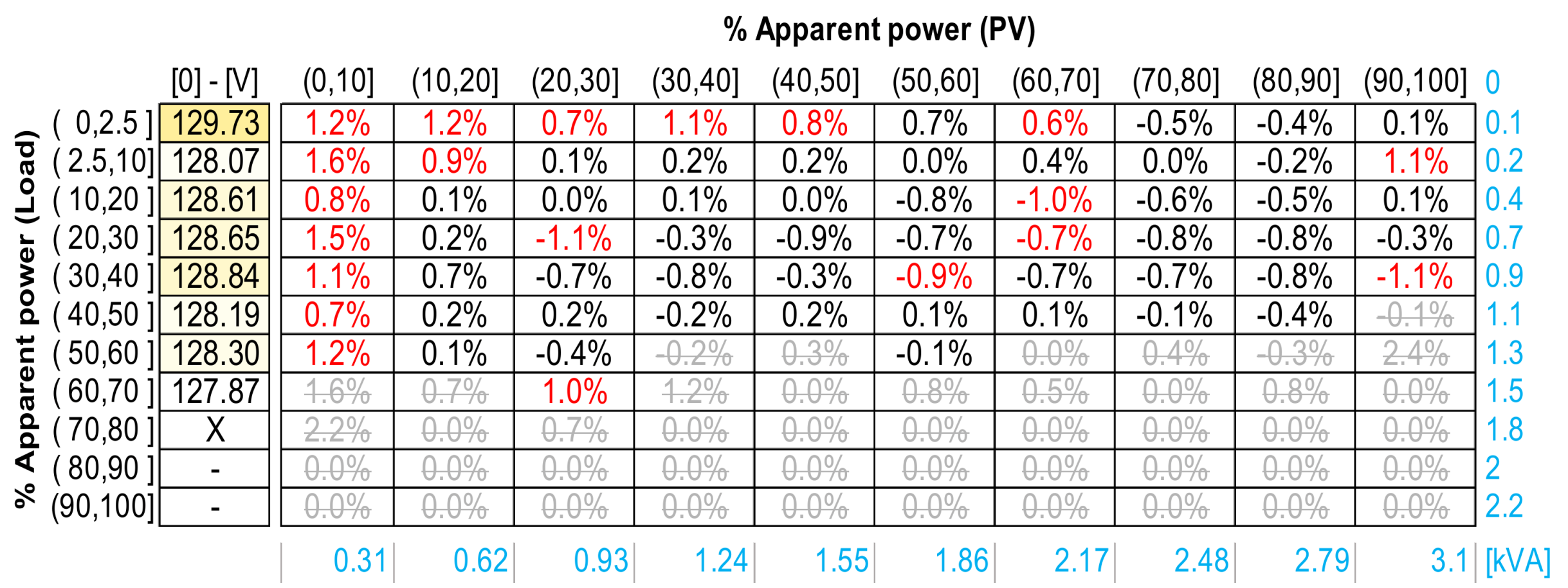
Figure 14, Figure 15 and Figure 16 show the average value of Vrms for each scenario considered for three phases. The first column corresponds to the values of Vrms without PV injection. Columns 2–11 show the values of Vrms for scenarios with PV power injection. The Vrms increased in almost all PV injection scenarios with loads between 0% and 2.5%, which partially coincides with the findings of Urbanetz et al. [15] who found that the effective voltage increased with high PV injection and a low load.

For example, the sampling population of V_{rms_A} for the $PVS Off(i=6)$ or (40, 50%) apparent power scenario had 78 data and a Vrms of 128.19 V, while the sample population of ${\mathrm{V}}_{\mathrm{rms}\_\mathrm{A}}$ for the $PVS On\left(6,3\right)$ scenario had 20 data and a Vrms of 128.49 V, which corresponds to an increase of 0.2%. However, the P-value was 0.296 and was obtained by applying the Wilcoxon rank sum test through the ‘ranksum’ function of MATLAB. As the P-value was greater than the 5% significance level, the null hypothesis was accepted. Therefore, there was no evidence to indicate a PV system impact on V_{rms_A}. Figure 17 shows the scenario matrix that relates the percentages of relative variation between a scenario with PV power injection (Columns 2–11) and a scenario without PV power injection for a range i.

The acceptance or rejection of the H₀ in each $PVS On\left(i,j\right)$ scenario is denoted in Figure 17 by coloured text: black, red, and grey to denote the acceptance of H₀, non-acceptance of H₀, and no application of the test because of an insufficient amount of data, respectively. In addition, a positive value apparently means that the parameter increased because of the PV injection, a negative may indicate that the parameter decreased because of the PV injection, an X value means there were less than four measurements for the scenario without PV injection, and the symbol ‘-‘ implies there were no measurements for the scenario without PV injection. The test was applied only when both injection scenarios with and without PV had sufficient data.

Table 5. Values of Vrms and results of the hypothesis testing for scenarios of greater probability for each phase.

Phase	Scenario	Load		PV Injection		${\mathit{V}}_{\mathit{r}\mathit{m}\mathit{s}\_\mathit{P}\mathit{V}\mathit{S} \mathit{O}\mathit{f}\mathit{f}\left(\mathit{i}\right)}$	${\mathit{V}}_{\mathit{r}\mathit{m}\mathit{s}\_\mathit{P}\mathit{V}\mathit{S} \mathit{O}\mathit{n}\left(\mathit{i},\mathit{j}\right)}$	Variation	H0
A	I = 1; j = 1	(0–2.5%] 0–0.06 kVA		(0–10%] 0–0.31 kVA		129.09	131.22	1.2%	Rejected
	I = 1; j = 4	(0–2.5%] 0–0.06 kVA		(30–40%] 0.93–1.24 kVA			131.17	1.1%	Rejected
	I = 1; j = 3	(0–2.5%] 0–0.06 kVA		(20–30%] 0.62–0.93 kVA			131.18	0.7%	Rejected
B	I = 2; j = 1	(2.5–10%] 0.05–0.18 kVA		(0–10%] 0–0.31kVA		129.53	131.56	1.78%	Rejected
	I = 2; j = 4	(2.5–10%] 0.05–0.18 kVA		(30–40%] 0.93–1.24 kVA			130.37	0.77%	Rejected
	I = 2; j = 3	(2.5–10%] 0.54–0.72 kVA		(20–30%] 0.62–0.93 kVA			130.29	0.66%	Rejected
C	I = 1; j = 1	(0–2.5%] 0–0.04 kVA		(0–10%] 0–0.31 kVA		129.73	131.40	1.53%	Rejected
	I = 1; j = 2	(0–2.5%] 0–0.04 kVA		(10–20%] 0.31–0.62 kVA			131.07	1.30%	Rejected
	I = 1; j = 4	(0–2.5%] 0–0.04 kVA		(30–40%] 0.93–1.24 kVA			130.89	0.77%	Rejected

relates the results of the hypothesis testing for the three most likely scenarios. The rejection of H₀ means that PV injection affect the profile average voltage. The Vrms increased for the entire PV injection range, although these variations was only between 0.66% and 1.78% and the parameter remained within the limits of the regulations. Such an increase at the PCC was also described by Urbanetz et al. [9], Farhoodnea et al. [10], Ahmed et al. [17], and Grycan et al. [18]. Nevertheless, results also indicate that PV injection only affect 33%, 45%, and 27% of the scenarios of phases A, B, and C.

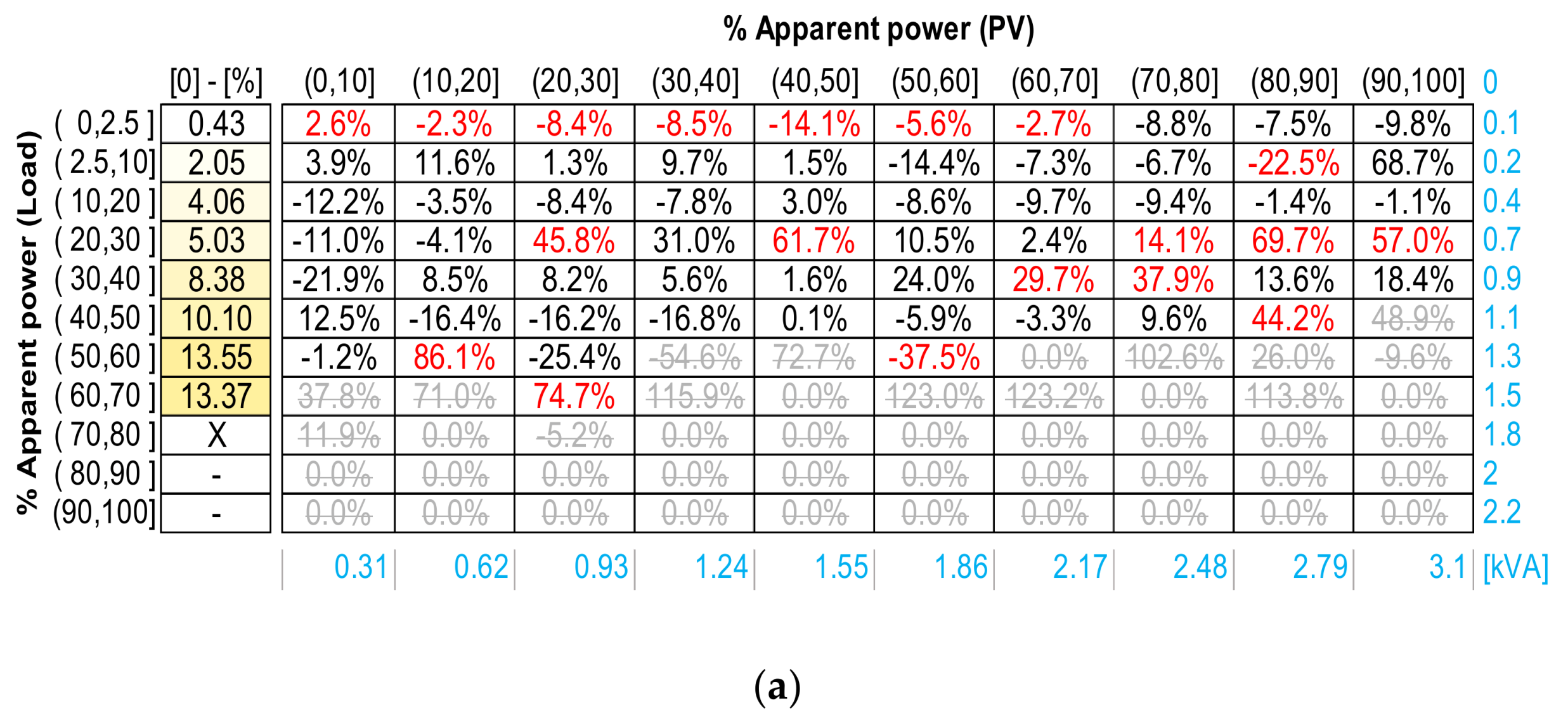
The TDD behaviour was proportional to the size of the connected load. Figure 18 shows that low load, as 0%–2.5%, can affect several scenarios by the PV injection in Phase A; however, these variations were insignificant because of the low value of this parameter without PV injection (0.43%). The highest affectation of TDD reached values of 70%–86%; these results are similar to those of Etier et al. [15] and Grycan et al. [18] who reported a greater variation of TDD as the PV power increased.

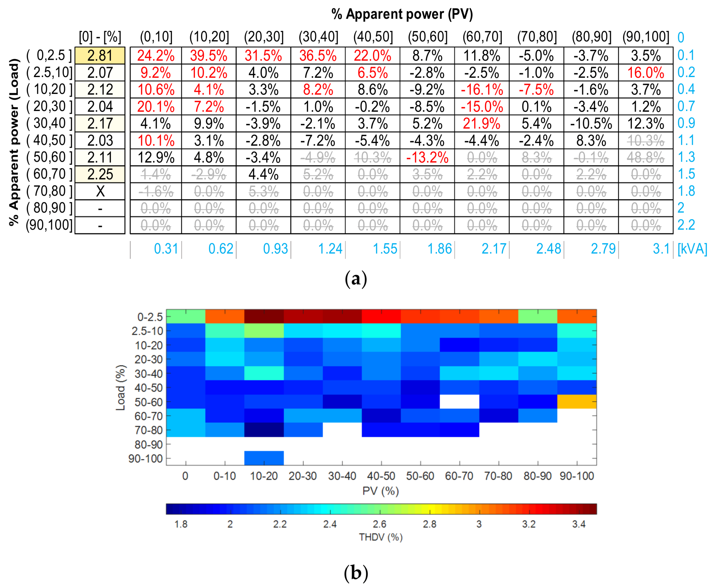
As shown in Figure 19, the THDV reached values up to 2.81% ($THD{V}_{PVS Off\left(1\right)}$) and 3.92% ($THD{V}_{PVS On\left(1,2\right)}$) for without and with PV injection for Phase A, both with lowest load power interval (0–2.5%). That means that low-load and low-PV injection conditions had a significant influence on the THDV, which indicates that THDV decreased as the PV injection increased and agreed with the results of Niitso et al. [13], Ahmed et al. [17], and Grycan et al. [18]. However, THDV values were always lower than the 8% limit (Table 2).

The total THDI reached values up to 185.74% ($THD{V}_{PVS Off\left(1\right)}$) and 191.1% ($THD{V}_{PVS On\left(1,2\right)}$) for without and with PV injection for Phase A, as shown in Figure 20, for lowest load power interval (0-2.5%). In general, the average THDI values with and without injection were 46.84% and 38.86%, 46.79% and 49.99%, and 40.51% and 35.54%, for phases A, B, and C, respectively. There was no evidence of a decrease in this parameter with an increase in the PV injection as observed by Nemes et al. [20] and Leite et al. [19].

The third and fifth harmonic voltage distortions did not exceed the 5% allowed limit. These parameters showed a random behaviour, but there was insufficient evidence to show that they decreased when the PV power injection increased, as Ahmed et al. [17] and Grycan et al. [18] found. The behaviour of VH5 is shown in Figure 21.

As expected, the IHDIs were proportional to the load demand. The scenarios with low loads seemed to be the most affected by the PV power injection; however, different levels of PV injection affected the random-load scenarios in each phase. The behaviour of IH3 is shown in Figure 22.

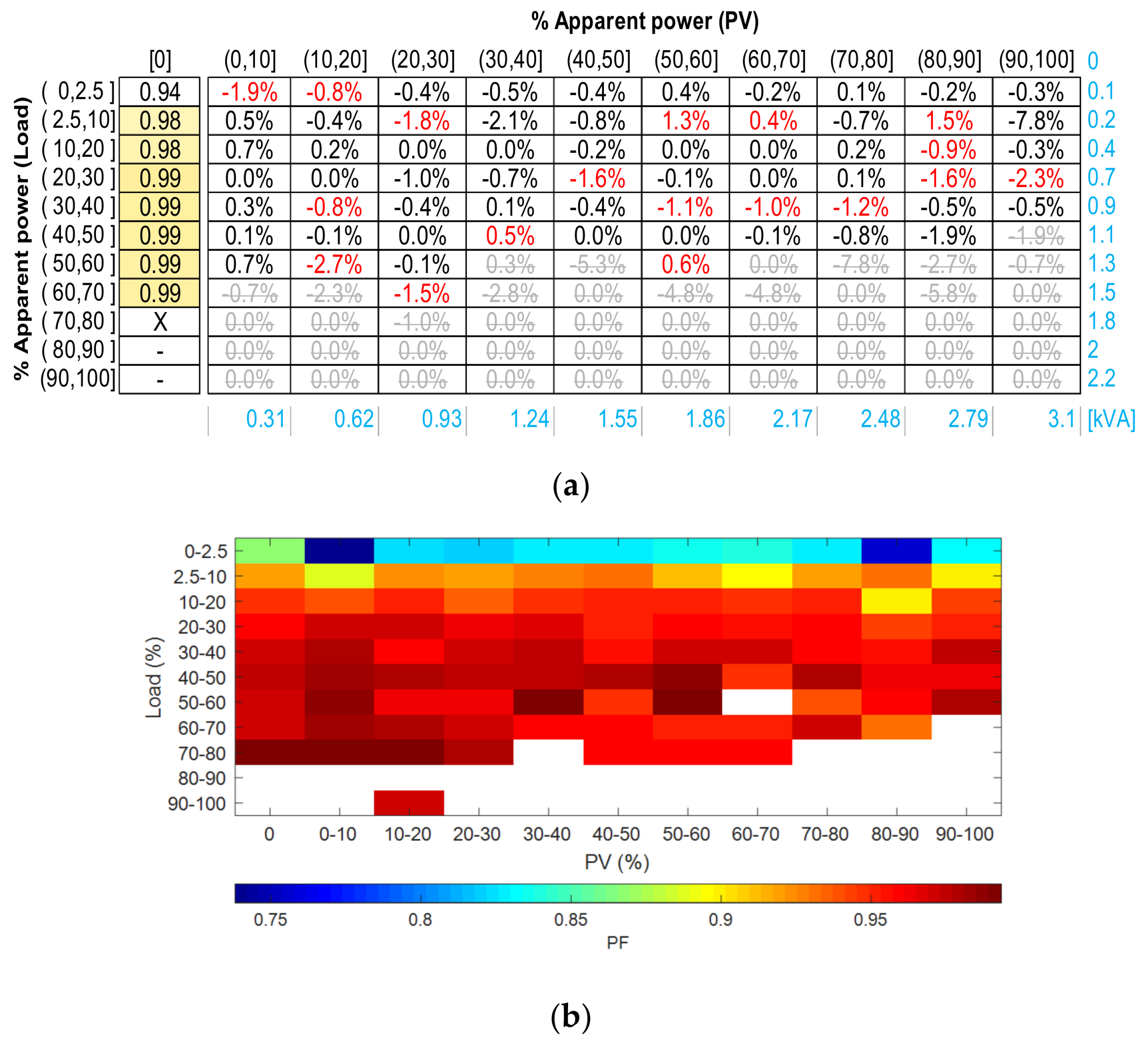
Figure 23 shows the slight impact of the PV system on the power factor where the maximum variation was 7.8%. The results showed random behaviour for several scenarios.

Figure 24 shows the impact of PV power injection on Pst. It appreciates that maximum variation is −23.4%, −35.6%. Most of scenarios with load intervals of 0%–2.5% and 30%–40% were affected by PV injection in Phase A.

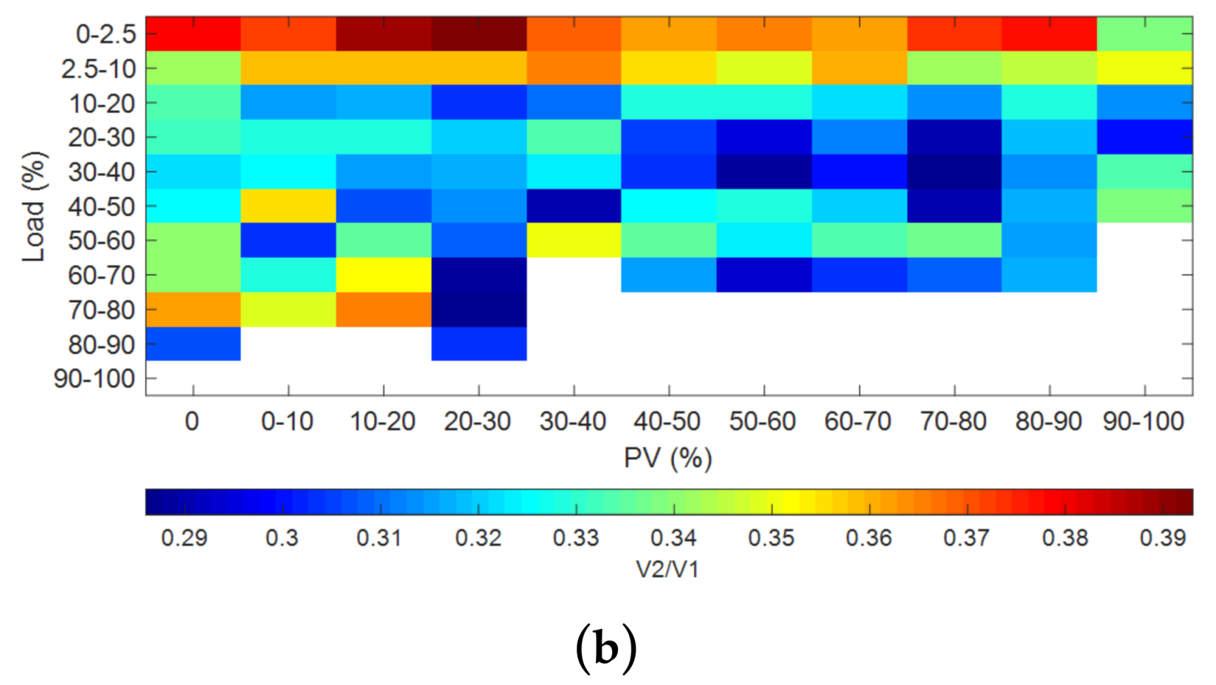
The voltage imbalance was analysed as a three-phase parameter; therefore, the values of apparent power in the scenario matrix were modified. Figure 25 shows that many scenarios were affected by loads between 2.5% and 30% with a PV injection between 0% and 70%. In addition, the scenario load presented the highest variation of imbalanced values, but it did not exceed 0.4%. In general, the voltage imbalance values were low and the variations with PV injection were insignificant.

Finally, it is possible to calculate the scale of the affectation caused by PV injection from percentage of affected scenarios, such as shown in Figure 26, which is mostly between 20% and 40%. The most affected parameters were VH3 with 51.56% of affected scenarios in Phase A, THDI with 51.47%, and IH3 with 48.53% in Phase C.

4. Conclusions

This study presents a methodology to quantify and evaluate the impact of PV integration on PQ, which applies the classification of data obtained through measurement using scenario matrices created by intervals of load power and PV injection. The study of the affectation of PV power injection is based on the application of hypothesis testing to compare two population means of the same parameter, one with PV injection and the other without PV injection, considering the same load power interval.

The application of the Kolgomorov–Smirnov (K–S) test, with a confidence level of 95%, showed insufficient evidence to accept the assumption of normality of the populations of the PQ parameters analysed. Therefore, the non-parametric Wilcoxon rank sum test was chosen to carry out the analysis of two independent sample populations.

Results obtained by the Wilcoxon rank sum test indicate that PV injection affects between 20-40% of scenarios of the PQ parameters analysed. Specifically, PV injection can cause an average variation on Vrms (+ 1.0%), TDD (- 4.2%), THDV (+ 32.4%), and VH5 (+ 16.5%), with a confidence level of 95%, for the load interval of 0–2.5% and PV injection intervals of 0–40%.

This study represents a step towards a better understanding of the affectation caused by PV power injection on power quality of the electrical networks. The insights developed will facilitate the positive integration of PV systems to LV networks. In addition, it is important to deepen the study of the application of normality tests and hypothesis testing for data obtained through measurements, the interaction between inverters and nonlinear loads, and the simultaneously affectation of PQ parameters on PCC and other nodes from networks.