Development and Assessment of an Integrated 1D-3D CFD Codes Coupling Methodology for Diesel Engine Combustion Simulation and Optimization

Abstract

In this paper, an integrated and automated methodology for the coupling between 1D- and 3D-CFD simulation codes is presented, which has been developed to support the design and calibration of new diesel engines. The aim of the proposed methodology is to couple 1D engine models, which may be available in the early stage engine development phases, with 3D predictive combustion simulations, in order to obtain reliable estimates of engine performance and emissions for newly designed automotive diesel engines. The coupling procedure features simulations performed in 1D-CFD by means of GT-SUITE and in 3D-CFD by means of Converge, executed within a specifically designed calculation methodology. An assessment of the coupling procedure has been performed by comparing its results with experimental data acquired on an automotive diesel engine, considering different working points, including both part load and full load conditions. Different multiple injection schedules have been evaluated for part-load operation, including pre and post injections. The proposed methodology, featuring detailed 3D chemistry modeling, was proven to be capable assessing pollutant formation properly, specifically to estimate NOx concentrations. Soot formation trends were also well-matched for most of the explored working points. The proposed procedure can therefore be considered as a suitable methodology to support the design and calibration of new diesel engines, due to its ability to provide reliable engine performance and emissions estimations from the early stage of a new engine development.

1. Introduction

Diesel engine performance and emissions are strongly dependent on the fuel spray injection, in-cylinder mixture formation, and combustion processes. The highly demanding legislative and environmental targets mandatorily require a clear understanding of the interaction between the fuel spray, the in-cylinder swirling flow field, and the piston bowl, to characterize the combustion efficiency and the pollutant formation phenomena correctly. Therefore, reliable Computational Fluid Dynamics (CFD) simulations are of paramount importance to integrate experimental studies for an efficient optimization and design of new Diesel combustion systems. Furthermore, with the exponential increase of the computational power of Central Processing Units (CPUs), extremely detailed physical and chemical models can be run with an acceptable computational time, becoming fundamental in the first stages of the design and development phase. On one hand, properly calibrated 1D-CFD models can be considered as adequate to reproduce the engine behavior accurately with a minimum computational effort. However, the development of new engine designs can condition the engine behavior significantly (e.g., a new piston bowl shape affects combustion) and requires a new calibration with experimental data in order to guarantee a satisfactory level of accuracy. On the other hand, the use of a 3D-CFD numerical model with its strong predictive capability can be helpful in simulating new engine designs to avoid an expensive and time-consuming experimental campaign. It is worth pointing out that a 0D/1D multizone combustion model could provide satisfying results with the aim to optimize the fuel injection strategy, as Piano et al. show in [1]. In their study, a detailed 1D model of the fuel injector coupled with a 1D model of the engine is employed to minimize Brake Specific Fuel Consumption (BSFC) and Combustion Noise (CN) without exceeding the Brake Specific NOx (BSNOx) baseline value. However, 3D-CFD detailed combustion analysis becomes essential when a substantial reshaping of the combustion chamber is introduced or when the post injection potential in soot emissions reduction is evaluated [2]. In addition, the two different numerical approaches could be considered complementary; in fact, co-simulations exploit the strongest points of both approaches, minimizing their drawbacks. For example, in engine simulation, an interesting option could be the development of a 1D/3D-CFD coupled methodology: 3D approach to simulate the complex components and flow processes in the combustion chamber, and 1D approach to solve the intake and exhaust systems gas flow. Following this procedure the possibility to integrate fast running 3D-CFD simulations into a 1D model is proposed in some commercial codes, where the two simulations run in parallel exchanging flow information (i.e., fluid pressure, velocity, temperature, and composition) at every timestep at specified boundaries. This approach is quite common and straightforward and could be pursued for detailed modeling of components (e.g., manifolds, compressors, turbines, valves, etc.), where the flow contains significant 3D effects, or 3D flow results are of specific interest. Several authors have chosen this option to optimize the geometry of complex engine components such as intake manifolds [3,4,5] or innovative cooling systems [6]. The purpose of this study is to propose an alternative possibility of 1D/3D coupling: 3D-CFD simulations are implemented to perform a detailed combustion analysis, using the 1D models to provide time-varying boundary conditions (BCs), a reliable injection rate profile, and to estimate brake specific quantities and other global engine parameters. To obtain high-fidelity results from a 3D-CFD in-cylinder simulation, it is necessary to impose realistic pressure and temperature traces at the intake and exhaust ports, as well as the initial thermodynamic conditions and species mass fractions inside the cylinder region. The integration of a 1D complete engine model to generate boundary and initial conditions is a well-established procedure, adopted for different applications ranging from dual fuel combustion analysis [7,8], to the combustion characterization in a two-stroke opposed piston engine [9], to the detection of knock tendency in spark ignition engines [10,11], as well as to the study of alternative combustion modes in Diesel engines [12]. However, while 1D-CFD codes could be implemented to support several types of analysis as intake/exhaust system optimization, turbo matching or global engine performance assessment, they are characterized by a limited predictive capability as far as the combustion process is concerned, especially in case of complex injection schedules (e.g., multiple injections, post injection for soot oxidation). Differently, a stand-alone 3D-CFD simulation could be suitable for detailed combustion analysis, but it is generally limited to the description of in-cylinder phenomena. The aim of the present work is therefore the development of an integrated and automated procedure able to achieve a realistic Diesel engine combustion simulation, as suitable support to predict engine performance parameters and emissions estimations in the early-stage design phase of a new engine, when no experimental data are available. Pursuing this target, the coupling of 1D models with the 3D-CFD simulation is fundamental to provide reliable and accurate combustion data to the “global” 1D-CFD model and not only to characterize the 3D simulation with proper BCs.

In the first part of the present work, the simulation methodology is described in detail, dwelling on the different setups, the CFD models chosen and the coupling technique between the 1D and the 3D setups. The essential elements of the described approach are a reliable spray calibration methodology and a combustion model coupled with a detailed chemistry scheme, to correctly characterize the emissions formation phenomena. A reliable spray modeling is fundamental to predict the fuel spray formation process and how it affects the combustion processes and should be accurately validated, as can be seen in other researches [13,14]. Moreover, one of the main novelties integrated into the simulation setup is the presence of a detailed 1D model of the injector, extensively described in [15,16], to provide a realistic injection rate also in presence of complex injection schedule, which is one of the fundamental inputs of a reliable 3D-CFD analysis. The 1D environment is also employed as a primary workflow for the whole engine design to obtain realistic time-dependent BCs. Finally, the presence of a 3D-CFD results post-processing is integrated, not only to guarantee consistency with respect to experimental data in terms of in-cylinder pressure and heat release rate comparison, but also to evaluate global engine parameters such as brake specific quantities, even in the preliminary engine design phase. All the steps of the numerical analysis are connected in an automated procedure thanks to the use of in-house developed Linux scripts, which allows exchanging data between the 1D-CFD software and the 3D-CFD one.

The entire setup is validated against experimental data on three working points of the engine map representatives of a typical type approval driving cycle, also considering complex injection strategies with pilot and post injections. The possibility to investigate the mixing improvement, combustion, and pollutant emissions formation when using different injection strategies becomes very attractive using 3D-CFD [17,18], and an example of this type of optimization is illustrated in the second part of the work. At one working point, a further assessment is carried out, varying the post injection strategy in order to minimize the soot emissions, being an interesting application of the present methodology. Other future applications can be the capability to study the influence of different fuel injection system designs on the spray targeting, as Leach et al. have done in [19] or an appropriate description of the combustion process involving complex piston bowl geometries [20,21]. Indeed, since the in-cylinder air and fuel motion control the combustion process, affecting the NOx and soot formation, the present multidimensional model could be a powerful tool to support the development phase of new piston bowl shapes improving air and fuel mixing to achieve a better spatial distribution of the fuel, also for complex, multi-pulse injection schedules [1], which are nowadays of paramount importance to achieve the ultra-low engine-out emissions levels necessary to fulfill the legislation limits.

2. Methodology

The engine selected for this study is a 4-cylinder Diesel turbocharged engine for light-duty applications, featuring a common rail injection system and a high-pressure Exhaust Gas Recirculation (EGR) loop.

Table 1. Main design characteristics of the test engine.

Cylinders	4
Bore × Stroke	79.7 mm × 80.1 mm
Displacement	1.6 L
Compression ratio	16:1
Turbocharger	Single-Stage with Variable Geometry Turbine (VGT)
Fuel injection system	Common rail Max Rail Pressure 2000 bar
Rated power and torque	100 kW @ 4000 rpm 320 Nm @ 2000 rpm

provides more information about the engine.

The test engine features a re-entrant type of bowl design, shown in Figure 1 and it is equipped with an 8-holes solenoid injector.

In order to validate the simulation setup, three different engine working points were explored, two of which at part load and one corresponding to the rated power, as depicted in Figure 2 on the engine operating map and listed in

Table 2. Selected engine WPs.

Speed (rpm)	BMEP (bar)
1500	5.0
2000	8.0
4000	18.5

. The two part load points can be considered as representatives of operating conditions during the execution of type approval driving cycles, where the choice of the third working point was made to test the reliability of the numerical model also in high speed-high load conditions.

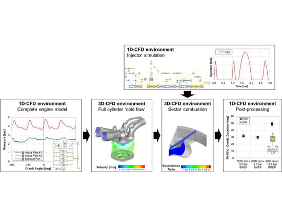
In the definition of a proper simulation setup for a compression ignition engine, the two fundamental needs are a well-calibrated spray modeling and an accurate combustion modeling. An automated coupling of 1D and 3D models was developed to address these requirements, and the adopted methodology is summarized in the block diagram of Figure 3. The 1D model of the entire engine runs separately respect to the two steps of the 3D simulations, to properly characterize the in-cylinder multidimensional simulation with suitable time dependent BCs in terms of pressure, temperature and species concentration. The entire engine cycle is simulated by means of a 1D complete engine model; in this work, a commercially available software GT-SUITE was selected and the validation results have been already presented in [22,23]. Results from this preliminary phase are used to initialize the first step of the 3D numerical analysis: a so-called full cylinder “cold flow” simulation. A cold flow analysis starts during the exhaust stroke up to the intake valve closure (IVC) to capture the thermodynamic conditions and the charge motion during the gas exchange process. Then, the combustion process is simulated considering only one sector of the cylinder centered on a single spray axis of the injector. The injector rate comes from a 1D injector model, extensively calibrated and validated in [15,16], in which the only input is the control current signal, in terms of Energizing Times (ET) and Dwell Times (DT). Finally, the results from the 3D combustion simulation are post-processed by means of a 1D post-process tool available in GT-SUITE environment, the Cylinder Pressure Only Analysis (CPOA). The CPOA is a stand-alone calculation starting only from the measured cylinder pressure, the engine geometry and basic operating cycle average results (such as volumetric efficiency and fuel injected mass). The boundary conditions needed from the CPOA and the pressure trace along the cycle are taken from the results of the 3D sector simulation. In this way, the simulated in-cylinder pressure is analyzed using the same solution methodology as the initial 1D engine model, ensuring perfect consistency between the 3D and the 1D approach. Moreover, the final output of the present methodology is the description of the engine performance in terms of global engine combustion parameters and emissions estimations. All the interconnections between the 1D engine model, the injector model, and the 3D two-stages simulation are performed automatically using in-house developed Linux scripts. The presence of automated interconnections between the different models allows the opportunity to implement the present methodology iteratively in a two-way coupling procedure: at the end of the first 3D-CFD simulation the obtained combustion data should be provided again to the 1D-CFD detailed engine model, setting up a new computational loop since the chosen convergence criteria would be satisfied. Even if in the present paper the iterative procedure is not proposed, it could be considered for future works.

2.1. D-CFD Simulation Setup

The complete engine model used in the first phase of 1D simulations is a detailed model of the entire engine, including all the subsystems as the turbocharger, the EGR circuit, all the pipes and volumes from the intake to the exhaust system. In this way, the model is able to reproduce the engine’s behavior accurately in all the different working points. The outputs obtained from the 1D model are imposed as boundary conditions in the 3D-CFD simulations. In detail, the temperature and pressure gas traces as a function of the crank angle and the value of the species mass fractions will be imposed at the intake and exhaust ports at the start of the subsequent 3D-CFD simulation, as well as the initial thermodynamics conditions and species mass fractions in the different regions in which the 3D cylinder model is divided. Finally, the results of the 3D sector combustion simulation are post-processed in a 1D model, to ensure consistency between the experimental data and the outcomes of the 3D-CFD simulation.

2.2. D-CFD Injector Simulation

An accurate and realistic injection profile is a fundamental input of the combustion 3D-CFD simulation. In this case, only a limited set of injection rates was available and to extend the availability of the model, there was the necessity to build a reliable injection rate profiles library. Therefore, a detailed 1D model of the solenoid injector was built in GT-SUITE [15,16]. The present injector model is able to calculate the injection rate starting from the Electronic Control Unit (ECU) parameters in terms of ET, DT and Rail Pressure.

2.3. D-CFD Simulation Setup

The 3D-CFD simulations are carried out using a commercially available software CONVERGE CFD, in two different steps. At first, a full cylinder cold flow simulation starts during the exhaust stroke until the IVC, to model the gas exchange process. This stage of the model aims to evaluate the thermodynamic conditions inside the cylinder, the gas exchange process, and the charge motion up to the end of the compression stroke, accounting for the interaction of the moving geometry with the fluid dynamics. As mentioned, the full cylinder simulation is automatically initialized using as time-varying boundary conditions the 1D-CFD complete engine model results. Then the 3D solution in terms of temperature, pressure, species concentration, and velocity field is mapped in all the cells of the domain at the IVC and imposed to a sector mesh to start the combustion simulation. The combustion simulation is performed only on a portion of the cylinder, on a sector of 45 degrees considering the presence of an 8-holes injector, as can be seen in Figure 4.

Simulating the combustion process only on a reduced volume of the entire cylinder geometry allows reducing the computational time significantly. This well-established simulation technique assumes that the swirl motion has a predominant effect, and therefore, the combustion process can be assumed as axial-symmetric [24]. A flat profile of the piston head is chosen hypothesizing that the presence of the valve seats does not affect the main outcomes of the combustion process considerably, as demonstrated by Bergin et al. in [25]. Since different sectors can give different results due to non-uniform charge distribution, the proper choice of the portion of the cylinder to be considered in the combustion simulation is performed comparing the results of different sector simulations with a combustion simulation carried out on the entire full cylinder geometry.

The base grid dimension in all the simulations is fixed at 0.5 mm, reaching the minimum size of 0.25 mm due to the two grid refinement techniques available in the 3D-CFD environment. Thanks to the high refinement of the base grid, a fixed embedding of the first level is considered adequate and is placed near the nozzle to depict the spray phenomena correctly. Apart from the near-nozzle region, it is quite challenging to choose a priori where a refinement of the grid is necessary. In this case, the Adaptive Mesh refinement (AMR) method is applied in all the sector volume, where high velocity and temperature gradients grow up and the grid is scaled according to the same abovementioned rules of the fixed embedding, as reported in [26].

As far as turbulence is concerned, the Reynolds-averaged Navier–Stokes (RANS) based Re-Normalization Group (RNG) k-ε model [27] is adopted. Considering the spray model, the atomization and the breakup of the droplets are calculated by means of calibrated Kelvin Helmholtz and Rayleigh Taylor (KH-RT) model [28]. The “blob” injection method of Reitz and Diwakar is used [28], in which parcels of liquid with a characteristic size equal to the effective nozzle diameter are injected into the computational domain. The O’Rourke model is chosen to simulate the turbulent dispersion of the spray parcels, distributing the parcels evenly throughout the cone of the injector [26]. The No Time Counter method (NTC) [29] is used as a collision model with the addition of a collision mesh and the dynamic droplet drag [30] to account for the possibility of variations in the drop shape. As far as the spray-wall interaction is concerned, the O’Rourke wall film model is adopted. Finally, the fuel evaporation is described by means of the Frossling evaporation model [31], which converts the evaporated liquid fuel mass into the specified source species. The validation of the spray model was done considering the breakup constants of the KH-RT model, the discharge coefficient and the spray angle values as calibration parameters, in comparison with penetration curves experimental data coming from constant volume vessel tests performed at the University of Perugia [32,33]. These data were available only for a reference injection, whose characteristics are shown in

Table 3. Main characteristics of the reference injection data.

Ref. Case–8-Holes	Solenoid Common Rail Injector
Vessel Pressure (bar)	11.28
Vessel Temperature (°C)	20
Rail Pressure (bar)	400
Energizing Time P2 (ms) ET-P2	0.215
Dwell Time P2 (ms) DT-P2	0.81
Energizing Time P1 (ms) ET-P1	0.21
Dwell Time P1 (ms) DT-P1	0.41
Energizing Time Main (ms) ET-Main	0.32

(see also Figure 5 for a sketch of the mentioned injection schedule).

Figure 5, top, shows the experimental injector current and injection rate profile used for the spray model calibration; the injection schedule presents two pilot injections and one main injection. To calibrate the breakup model, the constant volume vessel was reproduced in the 3D-CFD software and the injection rate was simulated by means of the 1D injector model. Figure 5, bottom, displays the results in terms of spray penetration of the three injections, comparing the numerical results with the experiments. A good agreement was found for the two pilot injections, while some differences can be seen in the case of the main injection. In this case, the discrepancies between the experimental and the simulated results could be addressed to the momentum transfer from the liquid jet to the air, and the corresponding possible local variations in the air density inside the test vessel in case of large injection pulses. For the purpose of this study, these results were considered acceptable according to the size of the baseline bowl (bowl radius approximately equal to 25 mm) and to the limited liquid spray penetration in real engine operating conditions. Further investigations could be carried out to more clearly understand the root causes of these discrepancies.

Concerning the combustion model, the SAGE detailed chemistry solver is implemented with the Skeletal Zeuch mechanism, the reduced version of the complete Zeuch mechanism, enhanced by the inclusion of soot reactions from Mauss’s work [34]. It features 121 species, including Poly-cyclic Aromatic Hydrocarbons (PAHs); therefore, it is possible to use the Particulate Mimic (PM) model [35], based on the method of moments, to predict the cell-averaged soot mass and number density. Since B10 fuel (10% biodiesel and 90% petrodiesel blend) was used for the experimental activity, in the numerical analysis the properties of the fuel are set equal to the ones of B10, as reported in

Table 4. Main characteristics of the B10 Diesel blend [36].

Characteristic	Method	Value
Density (at 15°)	EN ISO 3675	0.833 (kg/dm3)
Cetane Number	EN ISO 5165	54.2
Sulphur content	EN ISO 20,846	6.3 (mg/kg)
Lower heating value	ASTM D 240	42.32 (MJ/kg)
Higher heating value	ASTM D 240	45.20 (MJ/kg)
Stoichiometric air/fuel ratio	-	14.45

.

3. Results and Discussion

The discussed methodology was validated on three working points (see Figure 2 and Table 2) in terms of in-cylinder pressure and heat release rate, in comparison with the available experimental results. Firstly, the validation of the sector mesh simulation approach is presented in Figure 6, where the in-cylinder pressure obtained in the case of a full cylinder combustion simulation is compared with the results of the selected sector combustion analysis for the 4000 rpm, 18.5 bar of Brake Mean Effective Pressure (BMEP) WP. The comparison can be considered as acceptable since the sector simulation is able to reproduce correctly the entire combustion process allowing a noticeable advantage in terms of computational time saving, as highlighted in Figure 7.

Regarding the validation of the coupled 1D/3D approach, Figure 8 displays the comparison of experiments and numerical results for the working point 1500 rpm × 5.0 bar BMEP, where the injection profile from the 1D detailed injector model is highlighted in black dashed line. A good agreement is obtained, both in terms of in-cylinder pressure and heat release rate. The combustion timing is correctly captured by the numerical model for pilots, main and post injections.

The in-cylinder pressure and heat release rate compared with the experimental data are shown in Figure 9 for the second WP (2000 rpm × 8.0 bar BMEP). The combustion duration and the ignition delay are both correctly captured by the numerical simulation.

The capability of capturing the combustion process accurately is also confirmed in the last test engine working point, 4000 rpm × 18.5 bar BMEP, as shown in Figure 10, which features one pilot and main injection with high rail pressure, generally showing an excellent agreement between experiments and modeling results.

The excellent predictive capabilities of the proposed methodology could also be highlighted in Figure 11, in which the comparison between experiments and simulation results of the main combustion parameters is depicted. More specifically, the 3D-CFD sector simulation is able to predict Peak Pressure, Crank Angle (CA) at Peak Pressure, 10%–90% Combustion Duration and MFB50% with a high accuracy level. To further quantify the level of reliability of the simulation results,

Table 5. Absolute errors of the simulation results with respect to the experimental data for the main combustion parameters presented in Figure 11.

Engine WP	Peak Pressure	CA @ Peak Pressure	MFB 50%	10–90% Comb Duration
-	Error (bar)	Error (deg)	Error (deg)	Error (deg)
1500 rpm × 5.0 bar BMEP	+1.20	+0.11	−0.68	+1.29
2000 rpm × 8.0 bar BMEP	+2.08	−0.12	−0.62	−0.99
4000 rpm × 18.5 bar BMEP	−1.97	+0.30	+0.25	−2.28

shows the absolute error of the combustion parameters presented in Figure 11, with respect to the experimental data. For example, in terms of Peak Pressure, the error remains lower than +/−2 bar and can be considered as acceptable, as well as for the other combustion parameters.

Regarding the results in terms of pollutant emissions, Figure 12 shows normalized NOx emissions simulation results in comparison with experimental data. A very good agreement is noticeable in terms of trend across the three tested WPs. Concerning the soot values, Figure 13 presents normalized soot emissions comparing the experimental data with both empirical (Hiroyasu [37], blue bar) and detailed soot (PM, red bar) models. It can be highlighted that the empirical Hiroyasu model leads to a lower accuracy in soot prediction with respect to the detailed PM model. In fact, it is not able to capture the trend across the three WPs in terms of soot emissions, with a not negligible overestimation of the soot produced at the WP 1500 rpm × 5.0 bar BMEP. On the contrary, the PM model, supported by the detailed chemistry solver, depicts correctly the experimental trend. For these reasons, the detailed PM model was considered for the numerical soot prediction.

Thanks to the above described satisfactory validation of the proposed methodology, it can be considered as a valuable tool to scrutinize and optimize different combustion chamber and injector nozzle designs, also for complex multiple injection strategies.

As a possible example of application of the proposed methodology, the effect of different injection parameters on post injection efficacy in terms of soot reduction has been investigated and reported in this work. Four different injection schedules have been analyzed on a single working point (1500 rpm × 5.0 bar BMEP) varying either the timing or the post injected quantity, as shown in Figure 14. The Start of Injection (SOI) of the main and of the two pilot injections is kept constant. Moreover, the amount of fuel injected in the main injection is adjusted so to keep the engine BMEP at a constant level; this means that, at constant rail pressure, the main injection duration is reduced once the post injected quantity is increased, causing a longer post event. The injector detailed model is used to obtain the different injection profiles. As shown in Figure 14, the different injection schedules tested include a sweep of DT (600, 1000, 1400 μs) and a sweep of ET (170 and 210 μs).

The in-cylinder pressure and the simulated heat release rate are shown in Figure 15 considering the DT sweep. The predictivity of the numerical model can be considered as acceptable, although the model seems to slightly underestimate the heat release of the main injection for all the three cases, while slightly overestimating the heat release of the post injection for the post injections with higher DTs (case c and d). Moreover, the model seems to be unable to correctly predict the heat release of the post injection with the shorter DT (case a), suggesting that the effects of pulse to pulse interactions in terms of air and fuel mixing are not fully captured.

In Figure 16, the results obtained with a constant DT (600 μs) and different ETs of the post injection (case a vs. case b) are presented. Although the same discrepancies previously highlighted between the experimental and simulated heat release rate of the post injection could be pointed out, the overall evolution of the combustion process seems to be reasonably captured by the model, and further analysis, which will be described in the following paragraphs, will confirm its predicting capabilities.

The soot emissions results for the four post injection strategies analyzed are shown in Figure 17. Although the discrepancy between experimental and simulation results is quite evident in absolute terms, the simulation is capable to correctly capture the main trends among the different post injection strategies, highlighting that:

• the shorter post injection event is more effective in terms of soot emission reduction (soot emissions of case a are less than a half of soot emissions of case b);
• the influence of the post injection timing is definitely less important than the effect of the post injection quantity (soot emissions of case a, c and d, corresponding to different DTs, are comparable to each other, while are all significantly lower than soot emissions of case b, corresponding to a higher post injection quantity).

In order to more clearly understand the phenomenon, two different post injection schedules were selected and analyzed, with constant Dwell Time (DT = 600 µs) and different Energizing Times of the post injection event (ET = 170 and 210 µs, respectively), corresponding to case (a) and case (b) of the test matrix of Figure 14. The numerical results related to the injection rate (top), the heat release rate (center) and the time-varying total soot mass (bottom) of the chosen injection schedules are shown in Figure 18.

Firstly, it can be highlighted that the two curves of the total soot mass start to diverge during the post injection event, and the case with the higher post injected quantity (case b) presents the lower peak of total soot mass, probably due to the shorter main injection event. At the same time, the oxidation process appears to be more effective and faster for the case with the lower post injected quantity (case a). More in detail, the mechanisms of soot formation and oxidation have been investigated at four different crank angle degrees highlighted in Figure 18, analyzing the contour plots of the temperature, of the Turbulent Kinetic Energy (TKE), and of the soot mass distribution as reported in Figure 19, Figure 20, Figure 21 and Figure 22, respectively. The selected plane of the combustion chamber where the contour plots are presented is placed on the spray axis, corresponding to the middle of the sector geometry used to perform the 3D combustion simulation, as shown in Figure 19.

• At θ₁ = 10 deg aTDCf –2 deg CA after the start of the post injection events
  As shown in Figure 18, during the post injection events the soot mass curves of the two different injection schedules start to diverge, with a higher soot production in the case with shorter post injection (case a), which corresponds to a longer main injection. However, at this stage of the combustion process, the two cases are still showing almost identical soot masses, as confirmed by the contour plots of Figure 22, which do not yet show significant differences, although a higher temperature distribution in the spray area for case a) can be noticed in Figure 20, due to the more prolonged main injection (and, of course, combustion) event.
• At θ₂=15 deg aTDCf–3 deg CA after the end of the 210 µs post injection
  At this stage, looking at Figure 22, it is evident that the post injection with a shorter duration (case a) presents a higher production of soot within the bowl, while it shows a lower quantity of soot around the bowl rim. From the analysis of Figure 20 and Figure 21, it is quite evident that case b), due to the longer post injection, shows higher temperatures and higher turbulence intensities in the fuel spray jet and in the bowl rim regions, thus leading to a higher soot mass concentration in these regions. Nevertheless, the total quantity of soot at this CA remains higher for case a), being the soot production within the bowl clearly predominant.
• At θ₃=30 deg aTDCf–18 deg CA after the end of the 210 µs post injection
  Going ahead in the combustion process, the soot concentration for case (b) is significantly higher than for case (a) as shown in Figure 18, suggesting a faster and more effective oxidation process for case (a) (shorter post injection). This phenomenon is confirmed by the contour plots of Figure 22, where the amount of soot mass within the bowl is clearly lower for case (a) respect to case (b). The faster and more effective oxidation of the soot for case (a) can be attributed to a more intense mixing within the bowl, as shown by the higher TKE values in this region in Figure 21, and is further confirmed by the temperature contour plot of Figure 20, which displays a wider area of high temperatures.
• At θ₄=50 deg aTDCf–38 deg CA after the end of the 210 µs post injection
  Finally, when the final stage of the combustion is reached, the soot mass quantity for case (b) (longer post injection) remains higher, because the oxidation process in this case is less effective, as confirmed by the soot mass distributions of Figure 22, where a higher quantity of soot is evident in the upper part of the combustion chamber.

In conclusion, the detailed description of the in-cylinder phenomena, which can be provided by the 3D-CFD numerical simulation, appears to be a powerful tool for a thorough analysis and diagnosis of the combustion process also in case of new combustion chamber designs or in presence of complex injection schedules, which could affect the combustion and emissions formation phenomena significantly.

4. Conclusions

In this paper, an integrated methodology for the coupling between 1D- and 3D-CFD simulation codes has been presented. The proposed methodology aims to support the design and calibration of new diesel engines, coupling 1D engine models, usually available in the early stage engine development phases, with 3D detailed and predictive combustion simulations, respectively built in the commercially available software, GT-SUITE and CONVERGE CFD.

An assessment of the developed procedure has been performed by comparing its results with experimental data acquired on an automotive diesel engine, considering different working points, including both part load, and full load conditions. Besides, different multiple injection schedules have been evaluated for part-load operation, including pre- and post-injections and the proposed methodology has been proven to be capable of predicting the combustion and emissions formation processes for both NOx and soot emissions with satisfactory accuracy, also thanks to the integration of a detailed soot model.

The proposed procedure can, therefore, be considered as a suitable methodology to support the design and calibration of new diesel engines, thanks to its capability to provide reliable engine performance and emissions estimations from the early stage of new engine development.