Article

Optimization Model for Biogas Power Plant Feedstock Mixture Considering Feedstock and Transportation Costs Using a Differential Evolution Algorithm

1
Department of Computer Science and Information Technology, Faculty of Electrical Engineering, Josip Juraj Strossmayer University of Osijek, 31000 Osijek, Croatia
2
Enconsys d.o.o., 31000 Osijek, Croatia
3
Faculty of Economic Science, Institute of Regional and Agricultural Economics, Kaposvár University, H7400 Kaposvar, Hungary
*
Author to whom correspondence should be addressed.
Energies 2020, 13(7), 1610; https://doi.org/10.3390/en13071610
Submission received: 25 February 2020 / Revised: 29 March 2020 / Accepted: 30 March 2020 / Published: 1 April 2020
(This article belongs to the Section L: Energy Sources)

Abstract

:
In this paper, an optimization model for biogas power plant feedstock mixture with respect to feedstock and transportation costs using a differential evolution algorithm (DEA) is presented. A mathematical model and an optimization problem are presented. The proposed model introduces an optimal mixture of different feedstock combinations in a biogas power plant and informs about the maximal transportation distance for each feedstock before being unprofitable. In the case study, the proposed model is applied to five most commonly used feedstock in biogas power plants in Croatia and Hungary. The research is performed for a situation when the biogas power plant is not owned by the farm owner but by a third party. An optimization procedure is performed for each scenario with a cost of methane production that does not exceed 0.75 EUR/m3 in 1 MWe biogas power plant. The results show the needed yearly amounts and the maximum transportation distance of each feedstock.

Graphical Abstract

1. Introduction

Today’s world’s development is mostly based on fossil fuels. Due to the negative impact of fossil fuels on the environment and their limited reserves, the last decades have seen the use of renewable energy sources increase. According to References [1,2], installed capacity of renewable energy source (RES) for electricity generation has been increasing every year. In 2004, the total installed capacity of RES for electricity generation was 85 GW (or 800 GW when considering large hydro power plants), while it was 1081 GW by the end of 2017 (or 2195 GW when considering large hydro power plants). In 2016, the share of RES in the electric energy consumption was 24.5% [3], compared to 26.5% in 2017 [2].
For electricity generation (excluding large hydro power plants), the installed capacity of bio-power, geothermal, solar photo-voltaic (PV), concentrating solar thermal power (CSP), wind power and ocean energy capacity in 2017 was 122 GW, 12.8 GW, 402 GW, 4.9 GW, 539 GW and 0.5 GW, respectively [2]. From the previously mentioned RES technologies, geothermal and bio-power technologies have the highest capacity factors, as opposed to solar PV which has the lowest. Pursuant to Reference [4], the global weighted average capacity factors (CFs) for different renewable sources was constantly rising from 2010 to 2017, which indicates an increase in the yearly electricity generation per installed capacity.
This paper will focus on the biogas power plant based on anaerobic digestion. According to Reference [5], the total biogas power plant production was 62,704.00 GWh. Similarly, they [5] had the total annual energy generation of 181,565.00 GWh (electricity and thermal energy). Numerous biogas power plants in the European Union (EU) use agricultural feedstock. The European Biogas Association report for 2017 [5] gives an insight in used amounts of different feedstock combinations used in biogas power plants in the EU in 2016. Scarlat et al. [6] provide an overview of the RES policy, bioenergy and biogas markets, biogas production trends and biogas production in the EU. They [6] show that in 2015 in the EU, biogas delivered 127 TJ of heat and 61 TWh of electricity, which is about 50% of the total biogas consumption in Europe destined to heat generation.
If compared to other RES technologies such as PV systems, wind power plants or hydro power plants, which have variable (stochastic) electricity generation, biogas power plants’ electricity generation can be controlled and optimized. Biogas power plants can help in better integration of other RES technologies into the power system. According to Reference [7], flexible power provision from biogas power plants can significantly contribute to energy systems with high shares of renewables. In this paper, eight different indicators are defined to shape “flexibility” and perform a downstream investigation of eight research projects focusing on flexible energy provision of biogas plants. A new model of demand-driven supply by biogas power plants, which can offer a solution for more efficient integration of fluctuating supply of wind and solar energy, is presented in Reference [8]. The problem of operational planning of a biogas combing heat and power plant under the conditions of limited biofuel resources is analyzed in Reference [9]. Furthermore, biogas power plants can help improve the power quality in power grids with a high share of PV systems, such as that presented in Reference [10].
The recent increase of investments in biogas power plants in the EU is inspired by European and national policies. One of the goals of European climate and energy strategies is to increase the share of RES [11,12]. National policies of different EU countries have different ways to support investments in biogas power plants as well as other RES technologies such as subsidies, feed-in tariffs, feed-in premiums, etc. Several researches were conducted to analyze the investments in biogas power. Menind and Olt [13] analyzed the investment in biogas power plants, asking five questions on the market energy price, existing supports for RES and investment risks before investing in biogas power plants. One of these questions is related to a buying energy price, which in this research is considered as one of the constraint data. Salerno et al., in Reference [14], presented a financial and economic evaluation of small biogas power plants focusing on the comparison of several incentive systems used over time. Their conclusions (based on the Italian case study) show that despite the obvious recent price reductions, investments in small biogas power plants (e.g., 250 kW, 300 kW) can still be attractive. An economic analysis for centralized and decentralized biogas power plants in order to find the optimal electric capacity is presented in Reference [15]. The Brazilian case study results demonstrate that biogas power plants with electric capacity of over 1 MW perform better than smaller plants. Additionally, it shows that in small-scale biogas power plants (<1 MW), the costs related to the transport of the feedstock on distances below 30 km do not significantly impact the economic analysis. A comprehensive analysis of the cultivation, harvesting and transportation impact on the feedstock price is presented in Reference [16]. An example of calculating the biomass potential for energy generation is presented in Reference [17].
Geographical information systems (GIS) can be very useful to determine the optimal allocations of biogas power plants as well as to assess the biomass potential on specific regions. In Reference [18], the analysis of the spatial distribution and available amounts of biomass feedstock for biogas generation are presented. GIS is used to find the optimal site locations, size and power of the biogas power plants in the southern regions of Finland, where the objective function is a minimum transport distance using local roadmaps. GIS, with the combination of the Analytical Hierarchy Process (AHP) and Fuzzy Weighted Overlap Dominance (FWOD) procedure, is used to identify the most suitable locations for building future biogas power plants, taking into account the most relevant criteria for the social, economic and political dimensions, as presented in Reference [19]. The assessment of the spatial availability of locally available feedstock for the biogas generation in Assam, India, using GIS is presented in Reference [20]. In the same paper, GIS is used to optimize a design of a biomass collection and transportation network. GIS, as a supporting tool for planning future biogas plants, is also used in References [21,22,23]. Valenti et al. [23] used the GIS-based model to calculate the spatial index of the feedstock mixture availability, and the presented results could help local decision makers to show the suitable areas for the installation of new biogas power plants. In Reference [22], a three-step approach that uses data collection, GIS-based analysis and technical and economic assessment was used to analyze and design the biogas power generation system. It can be applied to other regions.
As previously mentioned, most of the biogas power plants in the EU are based on agricultural feedstock and anaerobic digestion technology. The feedstock can originate from the direct neighborhood of the farm or it can be collected in different locations at some distance from it. Consequently, one of the challenges is to find an optimal mix of the feedstock as well as the feasible transportation distance to the biogas power plant. Prior to the collection feedstock process, it is important to test feedstock mixture with different ratios of available feedstock in order to get optimal mixtures with the highest biogas contribution, as presented by Valenti et al. in Reference [24]. Testing of different feedstock mixtures can contribute to more flexible solutions for the biogas generation in accordance with seasonal availability of different feedstocks [24]. However, the needed volume of bio-methane determined by the plant power (size) should be taken into account in this case.
Wolf et al. [25] used artificial intelligence methods to optimize a feedstock mix. Recently, different metaheuristic (nature-inspired) global optimization techniques such as Genetic Algorithm (GA) and Particle Swarm Optimization (PSO) have been used to perform optimization regarding the biogas plant operation. They used GA and PSO methods to optimize the feedstock mix in order to have a stable and efficient biogas production. Celli et al. [26] propose the usage of the GA method to find optimal biomass power plants’ distribution. This model is integrated in a Geographical Information System (GIS) in order to achieve better performance. A bio-economic model for the optimization of agricultural biogas supply chains using artichoke byproducts in existing plants is developed in Reference [27]. The model uses a linear programming approach with two objective functions (net present value and land use from energy crops). Mixed integer linear programming (MILP) was used in Reference [28]. The MILP-based model is used to determine the optimal location of potential biogas power plants as well as the optimal location of potential biomass storage sites, where the objective function is maximization of the profit. Modeling of the supply chain network in Reference [28] takes the set of biomass sites with the available amount of biomass, the set of candidate sites for supplying biomass to biogas power plants and candidate sites for biomass storage with defined maximum storage capacity into consideration. Mixed-integer programming is proposed in Reference [29] in order to find an optimal location of the hubs for the collection of feedstock to minimize operation costs of supply chains. However, due to the complexity of the constrained objective function involving mixed-integer variables, optimal solutions cannot be readily obtained. For this reason, an optimal solution is finally found using a GA in Reference [29]. The GA is also used to optimize biogas power plant power generation [30] and feedstock mix [31]. The research presented in Reference [32] describes the method which enables the assessment of possible scenarios regarding the supply of biogas power plants with feedstock, pursuant to stakeholders’ preferences. MILP is used for modeling possible scenarios with the lowest costs and shortest distances in the supply network, while Analytical Hierarchical Process (AHP) is used for the assessment of the different scenarios. For the assessment of the different scenarios using AHP, the following criteria are used: global cost, total traveled distance, emission of CO2 and technical feasibility of each scenario’s implementation. Here, the distances of feedstock are defined as input data for different scenarios and given in three values: 7.5, 15 and 22.5 km.
Following previous literature, there are many optimization models for a biogas power plant. However, these models do not provide estimates of the possible feedstock transportation distance to the biogas power plant nor do they propose the possible feedstock prices necessary to achieve the desired cost of biogas production. A situation in which the power plant owner produces the raw material himself is usually considered in the current literature. In comparison to such situation, the presented research describes the optimization procedure for the scenario in which the power plant is owned by a third party and the power plant owner has to purchase the feedstock on the market. The research is inspired by the real situation. Therefore, this paper aims to solve this problem. The challenge is to find the maximum transportation distances to the reactor as well as the necessary yearly amounts (masses) of the different types of feedstock in order to produce biogas at a specific cost while considering the nominal power of the biogas power plant. This paper contributes to the existing literature by developing an optimization model for biogas power plant feedstock mixture considering feedstock and transportation costs using a differential evolution algorithm. The proposed model is applied in a case study that takes into account the five most commonly used feedstock destined to biogas power plants in Croatia and Hungary [33].
The rest of the paper is structured as follows: the second section presents the model description including the mathematical model description and optimization problem definition. In the third section, the model is applied on the case study, while the fourth section concludes the findings.

2. Model Description

The proposed model is described in this chapter and illustrated in Figure 1. One of the goals of this model is to find the maximum distance to the reactor for each feedstock (for defined conditions) in order to produce methane at a defined cost and to find the optimal amounts of each one of them. In order to find optimum transportation distances and feedstock amounts, a differential evolution algorithm method is used.
The presented model considers a situation in which a biogas plant is owned by a third party [20].

2.1. Mathematical Modeling

This subsection introduces a mathematical description of the problem. The biogas power plant can collect different quantities of the feedstock from various locations. The total mass of the feedstock fed into the biogas reactor is calculated as follows:
m tfs = i = 1 n m i
where:
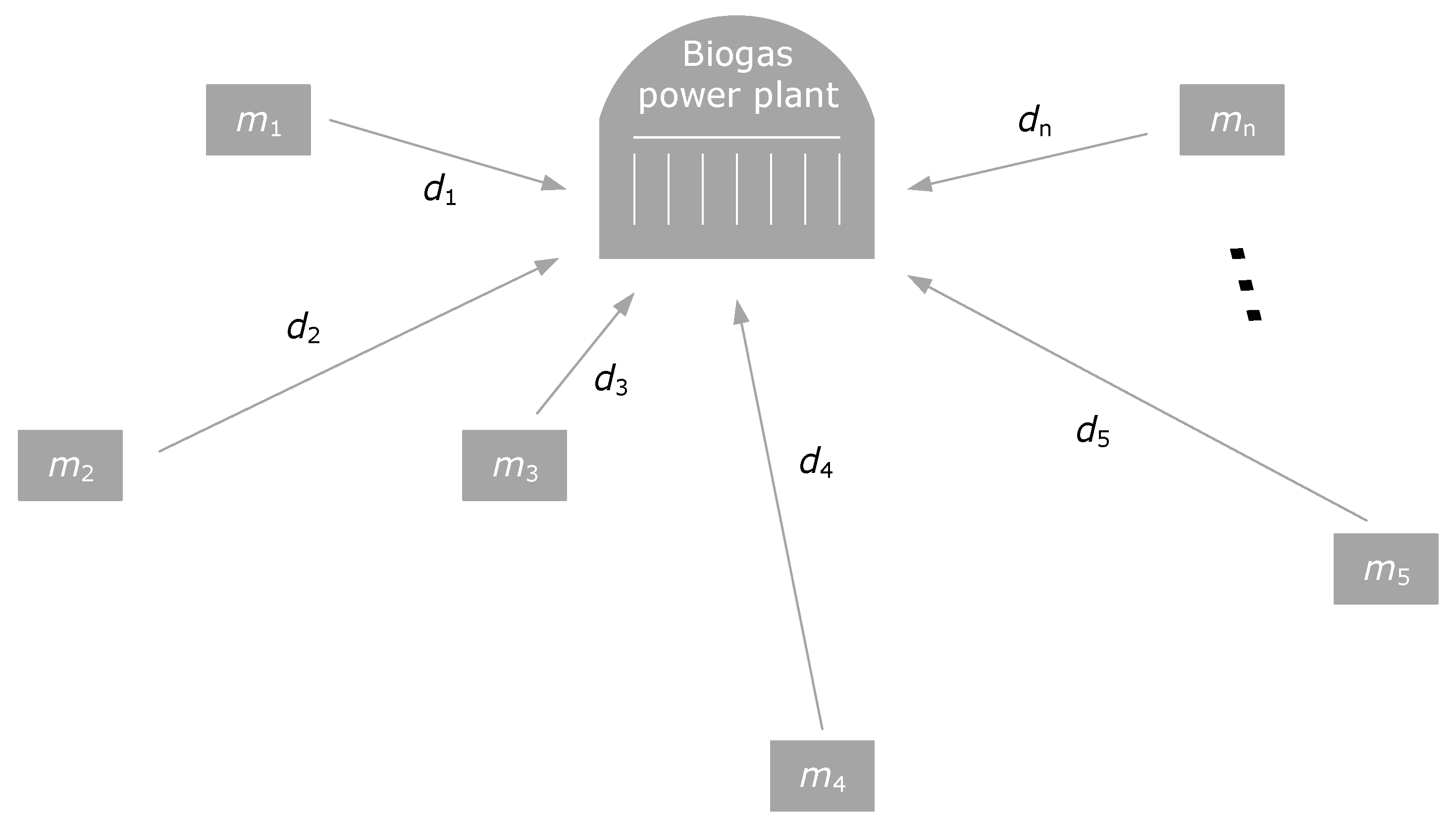
  • mtfs—total mass of the feedstock (t),
  • mi—mass of the i-th feedstock (t),
  • n—number of different feedstocks.
Since the total mass of the material consists of different density feedstock, the total volume of the feedstock must be calculated first. The following Equation can be used:
V tfs = i = 1 n m i ρ i
where:
  • Vtfs—total volume of the feedstock (m3),
  • ρi—density of the i-th feedstock (t/m3).
For the total amount of the feedstock, which contains different feedstocks, the total expected produced volume of methane is calculated as follows:
V methane = i = 1 n m i v i x i
where:
  • Vmethane—total volume of methane (Nm3),
  • vi—biogas yield of the i-th feedstock (m3/t of input),
  • xi—share of methane in 1 m3 of biogas expressed as a dimensionless relative number corresponding to the given percentage value.
The production cost of 1 m3 of methane is calculated as follows:
c methane = i = 1 n ( c i m i + c ti V i d i ) V methane
where:
  • cmethane—cost of 1 m3 of methane (EUR/m3),
  • ci—cost of the i-th feedstock (EUR/t),
  • cti—cost of the transport of the i-th feedstock (EUR/m3, km),
  • Vi—volume of the i-th feedstock (m3),
  • di—distance of the i-th feedstock for transportation (km).

2.2. Optimization Problem Definition and Objective Functions

The main goal of the presented problem is to find the feedstock’s maximal transportation distance for which the lowest possible methane production cost is achieved. The reciprocal values of the feedstock distances and the production cost of methane are used to aggregate the objective function of the minimization problem, such as:
OFv 1 ( d v ) = c methane c methane ,   max + i = 1 n d i , max d i
where dv is a vector of problem decision variables, cmethane,max is the upper limit of the methane production cost and di,max is the upper limit for transportation distance.
The additional optimizations are done by using objective functions that consider only distance or production costs:
OFv 2 ( d v ) = i = 1 n d i , max d i
OFv 3 ( d v ) = c methane
The decision variables of the optimization problem are masses and distances of the feedstocks, described as:
d v = [ m 1 m n d 1 d n ]
The general notation of the optimization problem is:
OFv i ( d v ) min ,   subject   to   constraints

2.3. Optimization Problem Constraints

The defined optimization problem has several practical constraints, as given below. Hydraulic Retention Time (HRT) is a constraint determined by a biological process in the digester of the biogas plant [34]. HRT impacts hydrogen and methane production and represents fermentation time in days [35]. HRT is calculated as the ratio of the reactor volume and the daily input volume of the feedstock [34]:
H R T = V reactor V input , d
Upon obtainment of the yearly amount of the necessary feedstock, the daily volume fed into the reactor is calculated by:
V input , d = V year 365
The constraint on HRT is defined as an inequality, such as:
H R T s , lower H R T s H R T s , upper
where HRTds. lower and HRTds. upper are the lower and upper limits for HRT (usually 50–60 days) and HRTs is the HRT value for a possible solution to the problem. This constraint ensures that the reactor is not emptied during the year, as it must remain full throughout the entire period.
The next constraint relates to the allowed dry matter content of the plant’s reactor. This constraint is important due to mixing and pumping problems. The author of Reference [36] points out that there is an upper limit for dry matter after mixing and pumping issues occur. In case of a high amount of the dry matter, energy demand for mixing and pumping (parasitic energy) will be increased [37]. Since the feedstocks need to be mixed continuously, during the biogas production process, the possible dry matter content is limited and must not exceed given values (depends on the mixing/pumping technology used). The dry matter content is calculated using Equation (13):
y = i = 1 n m i y i m tfs
where:
  • y—content of the dry matter expressed as a dimensionless relative number,
  • yi—content of the dry matter of the i-th feedstock, expressed as a dimensionless relative number corresponding to the given percentage value.
The dry matter content of the feedstock, calculated in the optimization procedure, is tested not to exceed the maximum allowed dry matter content depending on the mixing/pumping system used:
y y m a x
If the dry matter content of the feedstock mix exceeds this condition, water can be added for dilution. This constraint can be described with the following expression:
0.8 ( 1 y ) = 1 i = 1 n m i y i m tfs + m H 2 O
However, this water will use part of the reactor volume and the relation of the reactor volume to the total feedstock volume can be expressed as follows:
V reactor = V tfs + V H 2 O
where:
  • Vreactor—available volume of the reactor (m3),
  • VH2O—volume of water needed to achieve the maximum allowed content of the dry matter (m3).
The dry matter limit depends on the mixing/pumping system used, usually up to 15% [37,38] but according to the mixing/pumping system producers, the upper limit range is 10–45% considering the substrate type [39,40].
The availability (over a year) of different feedstock combinations is also considered in the form of an inequality constraint of the optimization problem:
M i M i , max
Furthermore, the maximal transportation distances of the feedstock are considered with the following constraint:
d i d i , max
The constraint that ensures that the plant produces its nominal power over the year depends on the required amount of methane produced per year. The calculated volumes of the produced methane have to be equal to the required methane volume, which represents the equality constraints. If the equality constraint is not satisfied, the penalization of the objective function is done for a very narrow range (to ensure practically the same amounts of methane) around the required methane volume for numerical reasons, in order to ensure convergence of the optimization procedure:
V methane = V methane , req OFv i = OFv i + | V methane V methane , req |   if   0.999 V methane , req V methane 1.001 V methane , req
The required methane volume per year is calculated based on the planned yearly electric energy production, as follows:
W Y = P n C F h Y
where:
  • WY—electric energy per year (kWh),
  • Pn—nominal plant power (electrical) (kW),
  • CF—capacity factor,
  • hY—planned number of working hours per year (h).
The primary energy is calculated as:
E p = W Y η
where:
  • η—efficiency of biogas power plant.
The required methane volume per year is:
V methane , req = E p H u
where:
  • Hu—heat value of methane (kWh/m3).
Moreover, the upper limit of the methane production cost is defined as a constraint of the problem. It must also ensure that the methane cost remains under a certain limit:
c methane c methane , max
The amount of cow manure in the total feedstock mix is expressed in Equation (24). This constraint is adapted to every specific feedstock:
r min m cm m tfs m r max

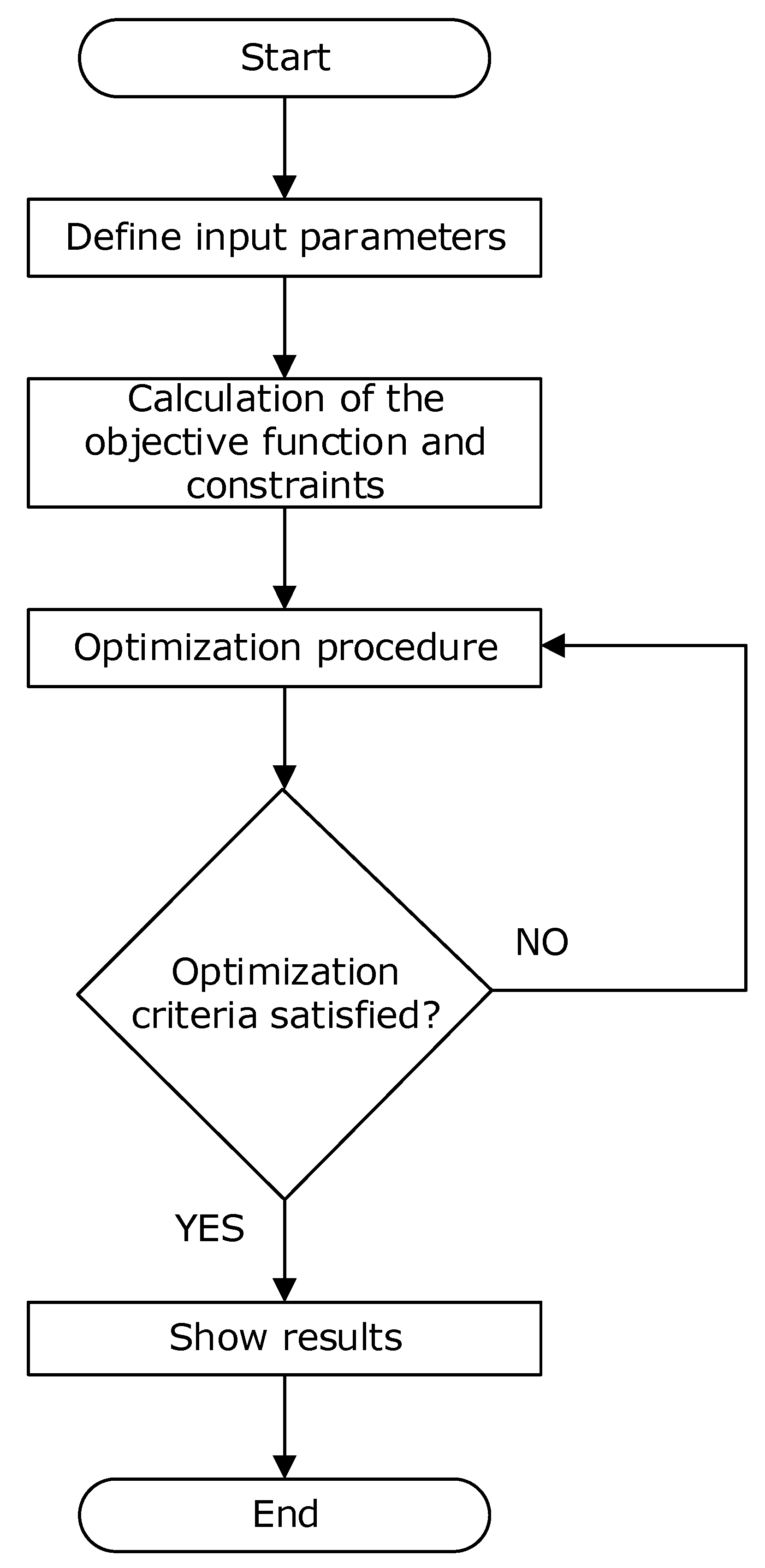
2.4. Optimization Method

A Differential Evolution Algorithm (DEA) is used to solve the optimization problem (Equation (12)) for the above-mentioned objectives (Equations (8)–(10)) and considering constraints (Equations (13)–(19), (23) and (24)). The existing DEA tool presented in the open-source scipy Python package (by SciPy.org) is used for this purpose. DEA has genetic operators (crossover, mutation and selection) similar to other types of evolutionary algorithms (EAs). The main difference with respect to other EAs is in a mutation operator, which is a difference between two possible solutions in DEA. The details about DEA can be found in Reference [41]. In Figure 2, a flowchart of the proposed optimization procedure is presented.

3. Results of the Case Study

In this case study, the application of the proposed model is presented. The model is used to find optimal transportation distances and different feedstock masses in order to produce biogas for the defined cost for a 1 MW biogas power plant. A mixture of the following five different feedstocks are considered for the biogas production: cow’s manure, cow’s slurry, pig’s slurry, millet silage and corn silage. These feedstocks are typically used in biogas power plants in Croatia and Hungary [5,33,34,42,43,44,45]. The constraint values used in the case study are given in Table 1. Table 2 and Table 3 list the input data for the case study’s proposed model. Different amounts of the dry and organic matters in some feedstock, as can be seen in the literature [43,46,47,48,49,50,51,52], are given. As it is pointed out in Reference [52], these data are usually: “…general, for exact values an individual substrate analysis has to be undertaken”. That being said, the data used in Table 2 are from Reference [53] (for millet silage, from Reference [51]) and are used here as an example to present the application of the proposed procedure. Normally, the proposed procedure can be used for any specific data depending on the given case. The feedstock price is subject to change [54] depending on the area market conditions and it can be defined during the contracting phase [53]. The price range can be pretty wide, e.g., 3.73–39.37 €/t for manure [53]. The feedstock prices given in Table 3 (column 5) are obtained from the plant owner in Croatia based on the local prices the owner used to pay for the feedstock. The similar prices for manure and silage in Hungary are presented in Reference [55]. These prices are used here to present the application of the procedure with numerical data, but any other prices can also be used in the model. The feedstock transport cost is not unique; rather, it depends on the local market and is negotiable between the plant owner and transportation companies. There are different models of the transportation costs. The cost is three-fold and it consists of fixed and variable (depends on distance) parts, such as in Reference [56], transportation cost defined for ranges of distances [57] or fixed cost [55]. The feedstock transport price model from Reference [56] is applied here with the coefficients obtained from the plant owner (column 6 in Table 3). These data are used as an example, but other data can also be used depending on given situations. In the case study, the impact of transportation distances on greenhouse gas (GHG) emissions and profit from digestate used as a fertilizer was not taken into account.
The feedstock and transportation price data given in Table 3 are used as a base case in the simulations given below. Several different objective functions of the optimization problem, given in Equations (5)–(7), are used in the case study. Some results and discussion are given below. The optimization procedure is repeated multiple times for each scenario to check convergence. Based on the optimization results, it can be concluded that the optimization problem (for each objective function) has a number of local optima. There are different optimal value combinations of the decision variables, showing that objective values are very close to each other. The ranges of possible solutions for the base case are shown in Figure 3, Figure 4 and Figure 5 in the form of boxplot graphs to visualize the existence of more different feedstock combinations. These data are obtained by repeating the optimization procedure 50 times for the same input data. The difference in the results are due to the stochastic character of the metaheuristic optimization method used.
The examples of the possible optimal values of the decision variables are presented in Table 4, Table 5 and Table 6 for Equations (5)–(7), respectively.
The ranges of decision variable values for Equations (6) and (7) are also obtained as in the case of Equation (5) (Figure 3, Figure 4 and Figure 5) but were not presented here due to space limitation. The impact of the objective function, feedstock and transportation cost will be elaborated on in the following sections.
In Figure 6, visualization of the results from Table 6 (solution 1) using QGIS (https://qgis.org/) are presented. The maximum distances from Table 6 using local roads are presented in Figure 6 as follows:
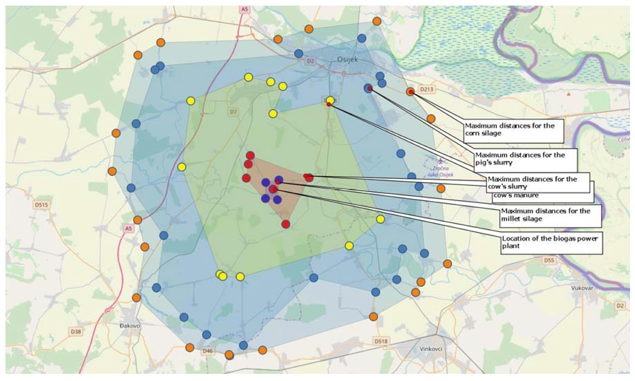
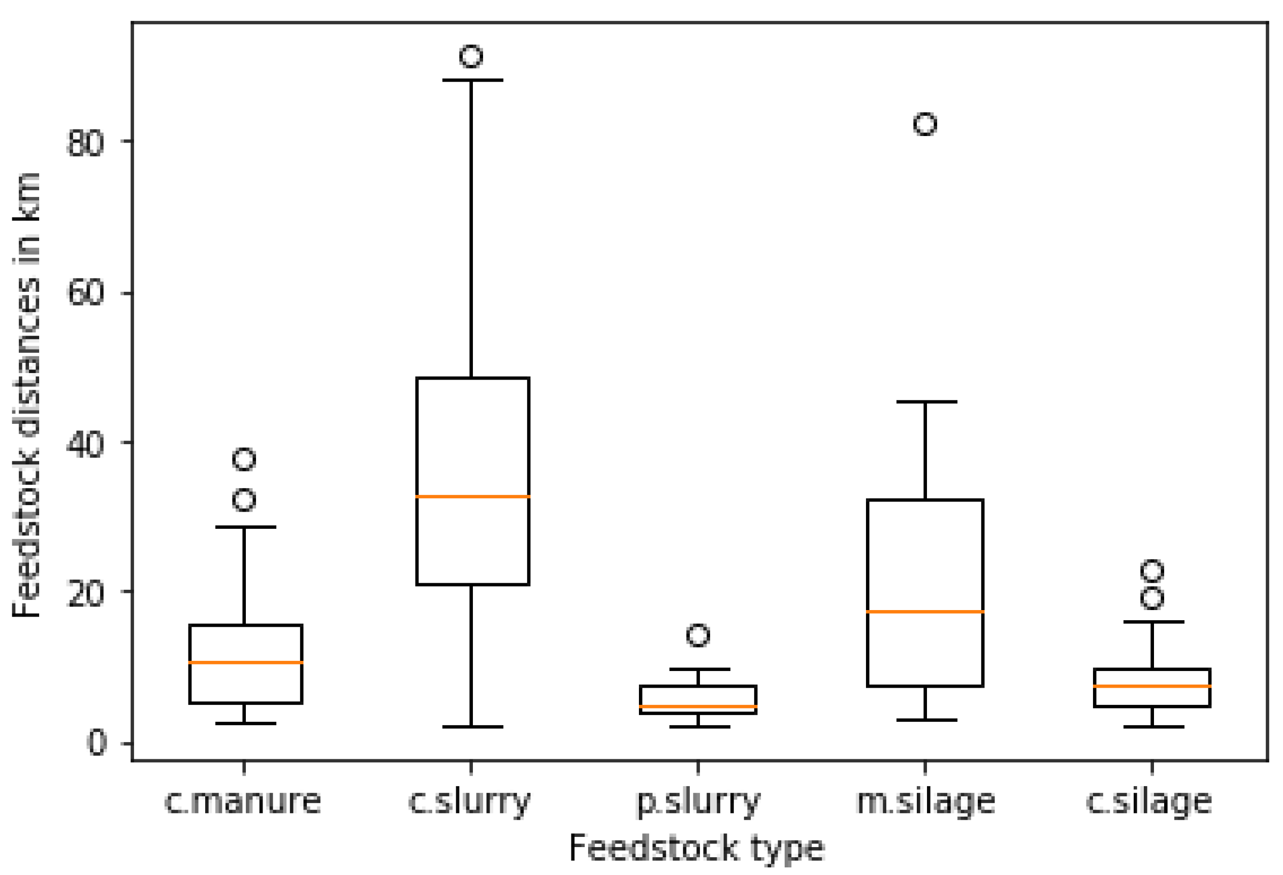
  • Purple circles represent the maximum distances for the collections of the cow’s manure using local roads,
  • Red circles represent the maximum distances for the collections of the cow’s slurry using local roads,
  • Yellow circles represent the maximum distances for the collections of the pig’s slurry using local roads,
  • Blue circles represent the maximum distances for the collections of the millet silage using local roads,
  • Orange circles represent the maximum distances for the collections of the corn silage using local roads.
In Section 2.2, three different objective functions were presented. In Figure 7, Figure 8 and Figure 9, the ranges of the methane production cost and decision variables, which depend on the objective function form, are presented.
Figure 7, Figure 8 and Figure 9 show that high distance for all feedstock types for Equations (5) and (6) can be achieved for the base values of input data. The main reason is the possibility to keep the methane production cost under the given limit of 0.35 EUR/m3 thanks to lower prices of the feedstock and transportation cost. In case of Equation (7), considering the bio methane production cost, only the upper limit distances for pig slurry and millet silage are lower than the upper limit and have values up to 56 and 24 km, respectively. For other feedstock, there are solutions including the highest distances.
The impact of increasing feedstock and transportation cost is illustrated below. In this scenario, the feedstock and transportation costs increased two and three times with respect to the base cost values. The simulation results for optimization repeated 50 times are presented in Figure 10, Figure 11 and Figure 12. The results for Equation (5) are given for the situation with the increased costs.
The situation proposing the increased feedstock and transportation costs and limited available volumes of the feedstock is simulated and elaborated on. The cost of feedstock and transportation increased two and three times of the base cost values, respectively. The limited volumes of cow slurry and millet silage in the amounts of 30% and 20% of the base limit values were used for the simulation purposes. The results are given in Figure 13, Figure 14 and Figure 15.
In case of the increased feedstock cost and limited available amounts, the ranges of the feedstock volume values for possible solutions are decreased (Figure 14) and maximal distances are limited to 50, 91, 25, 73 and 25 km for cow manure, cow slurry, pig slurry, millet silage and corn silage, respectively.
Figure 16, Figure 17 and Figure 18 present the results for the increased feedstock and transportation costs. Using Equation (7) (methane production cost minimization), the baseline values increased two and three times for the feedstock and transportation cost, respectively. In this case, most of the solutions find distances below 20, 50, 10, 40 and 10 km for cow manure, caw slurry, pig slurry, millet and corn silage, respectively. However, as can be seen, the solution including around 90 km for cow slurry and 80 km for millet silage can be found for a very narrow range of the methane production cost (0.61–0.62 EUR/m3, Figure 12).

4. Discussion

Based on the results shown in the previous section, the outcomes of the presented research are as follows:
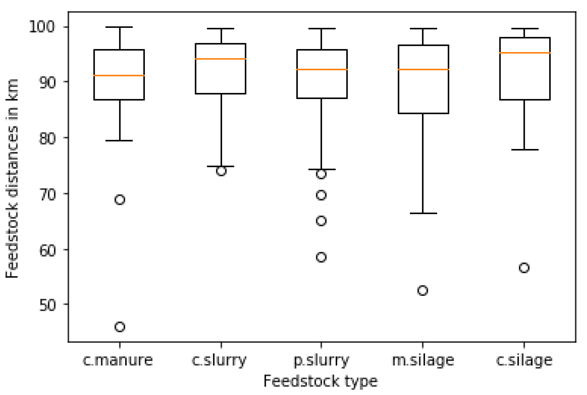
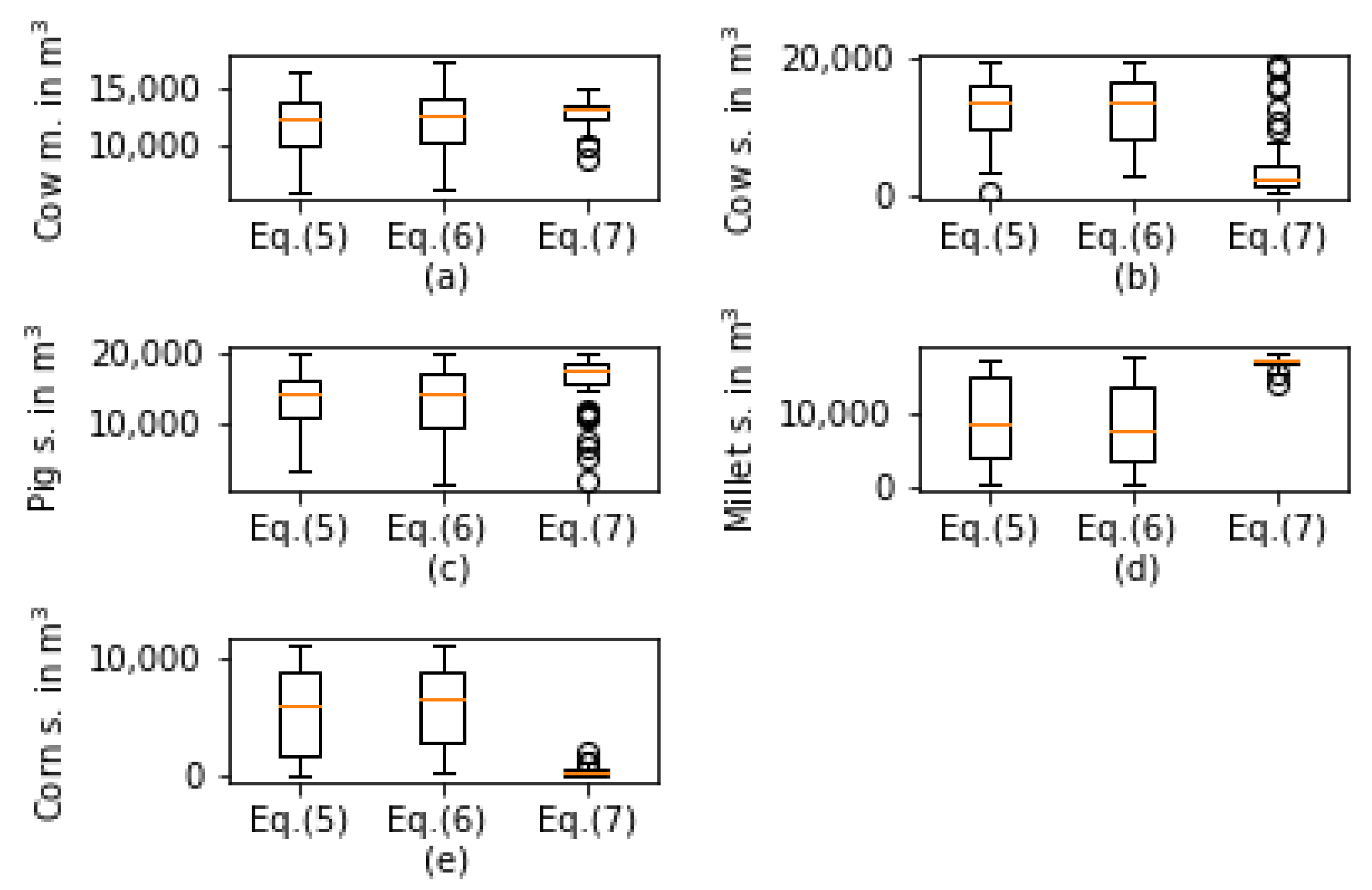
  • There are more different combinations of the feedstock volumes and distances which give very close values of the objective function values (for all three used objective formulations).
  • The upper distance limit for one feedstock depends on maximal distances of other feedstocks (Table 4, Table 5 and Table 6).
  • Using Equation (6) (including maximization of the distances only) enables us to find the upper limit of profitable feedstock distances considering the methane production cost constraint (Equation (23)) (profitable limit of the methane production cost).
  • The proposed procedure enables us to study the impact of different feedstock combinations and transportation prices according to the existing market prices and to determine the upper limit of the feedstock distances projecting the expected methane production cost.
  • The optimal mixture of feedstock can be found and used instead of only one feedstock type for minimization of the methane production cost.
The obtained maximum distances of feedstock are somewhat different than the values presented in the literature, especially for the base values of input data. The authors of Reference [59] stated that energetic break-even transportation distances for manure can be around 200 km; however, due to the economic criteria, they used 15 km distances in their research. The transportation distances up to 100 km or less (depends on a silage type) were found to be economically profitable in Reference [57]. Transportation distances from 0.5 to 3 km for different feedstock combinations were used in the scenarios presented in Reference [60]. According to Reference [45], transportation distances up to 10 km for manure are economically profitable for farmers and plant owners. In Reference [32], the feedstock distances are limited on the highest value of 22.5 km according to the real situation of the considered area. As can be seen from the obtained results as well as the reported values in the literature, the feedstock distances and volumes highly depend on the used model, cost assumptions and scenarios. A similar conclusion is given in Reference [57], where the authors stated that the direct comparison of results obtained through different studies cannot be always done due to differences in “… assumptions, economic contexts (e.g., public subsidy framework, feedstock prices, etc.) and assessment methods…”. The authors in Reference [61] acknowledged that different feedstock combinations depend on availability and feedstock prices. Furthermore, Valenti et al. [24] recommend that prior to the feedstock collection process, it is important to test feedstock mixture with different ratios of available feedstock in order to get the optimal mixtures with the highest biogas contribution. Based on the results presented in the previous section, it can be concluded that the proposed procedure can lead to finding not only one but also more solutions for defined constraints and input data.

5. Conclusions

In this paper, the optimization model for biogas power plant feedstock mixture considering feedstock and transportation costs using the differential evolution algorithm is presented. The model is applicable to find the maximum profitable transportation distance (for defined conditions) in order to produce biogas (methane) at the defined cost and to find needed yearly amounts (masses) of different feedstock combinations for the desired nominal power of the biogas power plant. In the case study, the proposed model is used to find the optimal mixture of five different feedstock combinations usually used in Croatia and Hungary for biogas production. The obtained results show that there are several solutions (combinations) meeting the given constraints; however, only some of them are elaborated on in this paper. According to the case study results, the solutions point to very close objective function values. This indicates that the optimization problem has numerous close local optima in this specific case. That being said, a preferable type of feedstock cannot be generally recommended. The presented procedure can be used as a useful tool to research different scenarios for purchasing of different feedstock combinations according to the current feedstock market offer. The presented procedure can be useful to determine the maximum cost-effective distances considering the price limit of the produced biogas. For this purpose, the presented procedure can be implemented in the tool for biogas plant operation planning (similarly, a tool for biogas plant investment can be found in References [62,63]) to simplify the direct use for plant owners. The obtained results show that one needs to be careful with defining the optimization problem objective because it has a significant impact on the optimal solutions. Further research can include the additional constraints and more detailed modeling of the biogas production (including the impact of transportation distances on greenhouse gas (GHG) emissions and profit from digestate used as fertilizer) in the presented optimization procedure. The presented procedure can be used for maximizing the distance of specific feedstock by changing the objective and problem constraints. This fact makes the presented model more general and useful for some other optimizations regarding the biogas production.

Author Contributions

Conceptualization, D.T. and D.M.; methodology, D.T. and M.B.; software, M.B. and D.T.; validation, D.M., C.M., D.T. and M.B.; resources, D.M. and C.M.; writing—original draft preparation, D.T. and M.B.; writing—review and editing, D.T., M.B., D.M. and C.M. All authors have read and agreed to the published version of the manuscript.

Funding

This research received no external funding.

Acknowledgments

This paper is a part of the project “Smart Specialization Programme of Kaposvar University No. EFOP-3.6.1.-16-2016-00007.

Conflicts of Interest

The authors declare no conflict of interest.

References

  1. REN21. Renewables 2014, Global Status Report; REN21: Paris, France, 2014. [Google Scholar]
  2. REN21. Renewables 2018 Global Status Report; REN21: Paris, France, 2018. [Google Scholar]
  3. REN21. Renewables 2017, Global Status Report; REN21: Paris, France, 2017. [Google Scholar]
  4. IRENA. Renewable Power Generation Costs in 2017; IRENA: Abu Dhabi, UAE, 2018. [Google Scholar]
  5. EBA. Statistical Report 2017; EBA: Brussels, Belgium, 2017. [Google Scholar]
  6. Scarlat, N.; Dallemand, J.F.; Fahl, F. Biogas: Developments and perspectives in Europe. Renew. Energy 2018, 129, 457–472. [Google Scholar] [CrossRef]
  7. Dotzauer, M.; Pfeiffer, D.; Lauer, M.; Pohl, M.; Mauky, E.; Bär, K.; Sonnleitner, M.; Zörner, W.; Hudde, J.; Schwarz, B.; et al. How to measure flexibility—Performance indicators for demand driven power generation from biogas plants. Renew. Energy 2019, 134, 135–146. [Google Scholar] [CrossRef]
  8. Rieke, C.; Stollenwerk, D.; Dahmen, M.; Pieper, M. Modeling and optimization of a biogas plant for a demand-driven energy supply. Energy 2018, 145, 657–664. [Google Scholar] [CrossRef]
  9. Varfolomejeva, R.; Sauhats, A.; Umbrasko, I.; Broka, Z. Biogas power plant operation considering limited biofuel resources. In Proceedings of the 2015 IEEE 15th International Conference on Environment and Electrical Engineering, EEEIC 2015—Conference Proceedings, Rome, Italy, 10–13 June 2015; pp. 570–575. [Google Scholar]
  10. Klaić, Z.; Knežević, G.; Primorac, M.; Topić, D. Impact of photovoltaic and biogas power plant on harmonics in distribution network. IET Renew. Power Gener. 2020, 14, 110–117. [Google Scholar] [CrossRef]
  11. European Comission, 2030 Climate & Energy Framework. Available online: https://ec.europa.eu/clima/policies/strategies/2030_en (accessed on 20 December 2019).
  12. European Comission, 2020 Climate & Energy Package. Available online: https://ec.europa.eu/clima/policies/strategies/2020_en (accessed on 20 December 2019).
  13. Menind, A.; Olt, J. Biogas plant investment analysis, cost benefit and main factors. In Proceedings of the 8th International Scientific Conference Engineering For Rural Development, Jelgava, Latvia, 28–29 May 2009; pp. 339–343. [Google Scholar]
  14. Salerno, M.; Gallucci, F.; Pari, L.; Zambon, I.; Sarri, D.; Colantoni, A. Costs-benefits analysis of a small-scale biogas plant and electric energy production. Bulg. J. Agric. Sci. 2017, 23, 357–362. [Google Scholar]
  15. Velásquez Piñas, J.A.; Venturini, O.J.; Silva Lora, E.E.; del Olmo, O.A.; Calle Roalcaba, O.D. An economic holistic feasibility assessment of centralized and decentralized biogas plants with mono-digestion and co-digestion systems. Renew. Energy 2019, 139, 40–51. [Google Scholar] [CrossRef]
  16. Stürmer, B.; Schmid, E.; Eder, M.W. Impacts of biogas plant performance factors on total substrate costs. Biomass and Bioenergy 2011, 35, 1552–1560. [Google Scholar] [CrossRef]
  17. Roberts, J.J.; Cassula, A.M.; Osvaldo Prado, P.; Dias, R.A.; Balestieri, J.A.P. Assessment of dry residual biomass potential for use as alternative energy source in the party of General Pueyrredón, Argentina. Renew. Sustain. Energy Rev. 2015, 41, 568–583. [Google Scholar] [CrossRef]
  18. Höhn, J.; Lehtonen, E.; Rasi, S.; Rintala, J. A Geographical Information System (GIS) based methodology for determination of potential biomasses and sites for biogas plants in southern Finland. Appl. Energy 2014, 113, 1–10. [Google Scholar] [CrossRef]
  19. Franco, C.; Bojesen, M.; Hougaard, J.L.; Nielsen, K. A fuzzy approach to a multiple criteria and Geographical Information System for decision support on suitable locations for biogas plants. Appl. Energy 2015, 140, 304–315. [Google Scholar] [CrossRef] [Green Version]
  20. Brahma, A.; Saikia, K.; Hiloidhari, M.; Baruah, D.C. GIS based planning of a biomethanation power plant in Assam, India. Renew. Sustain. Energy Rev. 2016, 62, 596–608. [Google Scholar] [CrossRef]
  21. Zubaryeva, A.; Zaccarelli, N.; Del Giudice, C.; Zurlini, G. Spatially explicit assessment of local biomass availability for distributed biogas production via anaerobic co-digestion - Mediterranean case study. Renew. Energy 2012, 39, 261–270. [Google Scholar] [CrossRef]
  22. Valenti, F.; Porto, S.M.C.; Dale, B.E.; Liao, W. Spatial analysis of feedstock supply and logistics to establish regional biogas power generation: A case study in the region of Sicily. Renew. Sustain. Energy Rev. 2018, 97, 50–63. [Google Scholar] [CrossRef]
  23. Valenti, F.; Liao, W.; Porto, S.M. A GIS-based spatial index of feedstock-mixture availability for anaerobic co-digestion of Mediterranean by-products and agricultural residues. Biofuels Bioprod. Biorefin. 2018, 12, 362–378. [Google Scholar] [CrossRef]
  24. Valenti, F.; Zhong, Y.; Sun, M.; Porto, S.M.C.; Toscano, A.; Dale, B.E.; Sibilla, F.; Liao, W. Anaerobic co-digestion of multiple agricultural residues to enhance biogas production in southern Italy. Waste Manag. 2018, 78, 151–157. [Google Scholar] [CrossRef]
  25. Wolf, C.; McLoone, S.; Bongards, M. Biogasanlagenregelung und -optimierung mit computational intelligence methoden. At-Automatisierungstechnik 2009, 57, 638–650. [Google Scholar] [CrossRef]
  26. Celli, G.; Ghiani, E.; Loddo, M.; Pilo, F.; Pani, S. Optimal location of biogas and biomass generation plants. In Proceedings of the 43rd International Universities Power Engineering Conference, Padova, Italy, 1–4 September 2008. [Google Scholar]
  27. De Menna, F.; Malagnino, R.A.; Vittuari, M.; Segrè, A.; Molari, G.; Deligios, P.A.; Solinas, S.; Ledda, L. Optimization of agricultural biogas supply chains using artichoke byproducts in existing plants. Agric. Syst. 2018, 165, 137–146. [Google Scholar] [CrossRef]
  28. Balaman, Ş.Y.; Selim, H. A network design model for biomass to energy supply chains with anaerobic digestion systems. Appl. Energy 2014, 130, 289–304. [Google Scholar] [CrossRef]
  29. Sarker, B.R.; Wu, B.; Paudel, K.P. Modeling and optimization of a supply chain of renewable biomass and biogas: Processing plant location. Appl. Energy 2019, 239, 343–355. [Google Scholar] [CrossRef]
  30. Araoye, T.O.; Mgbachi, C.A.; Omosebi, O.A.; Ajayi, O.D.; Olaniyan, A.Q. Development of a Genetic Algorithm Optimization Model for Biogas Power Electrical Generation. Eur. J. Eng. Res. Sci. 2019, 4, 7–11. [Google Scholar] [CrossRef]
  31. Wolf, C.; McLoone, S.; Bongards, M. Biogas plant optimization using genetic algorithms and particle swarm optimization. In Proceedings of the IET Irish Signals and Systems Conference (ISSC 2008), Galway, Ireland, 18–19 June 2008; Volume 1, pp. 244–249. [Google Scholar]
  32. Galvez, D.; Rakotondranaivo, A.; Morel, L.; Camargo, M.; Fick, M. Reverse logistics network design for a biogas plant: An approach based on MILP optimization and Analytical Hierarchical Process (AHP). J. Manuf. Syst. 2015, 37, 616–623. [Google Scholar] [CrossRef]
  33. BiogasAction—New Developments in Croatia. Available online: https://www.fedarene.org/biogasaction-new-developments-croatia-23048 (accessed on 25 January 2020).
  34. Müller, F.; Maack, G.C.; Buescher, W. Effects of Biogas Substrate Recirculation on Methane Yield and Efficiency of a Liquid-Manure-Based Biogas Plant. Energies 2017, 10, 325. [Google Scholar]
  35. Mohan, S.V.; Mohanakrishna, G.; Srikanth, S. Biohydrogen production from industrial effluents. In Biofuels; Elsevier Inc.: Amsterdam, The Netherlands, 2011; pp. 499–524. ISBN 9780123850997. [Google Scholar]
  36. Hughes, K.L.W. Optimisation of Methane Production from Anaerobically Digested Cow Slurry Using Mixing Regime and Hydraulic Retention Time; University of Exeter: Exeter, UK, 2015. [Google Scholar]
  37. Brambilla, M.; Romano, E.; Cutini, M.; Pari, L.; Bisaglia, C. Rheological Properties of Manure/Biomass Mixtures and Pumping Strategies to Improve Ingestate Formulation: A Review. Trans. ASABE 2013, 56, 1905–1920. [Google Scholar]
  38. Biogas—Feedstocks. Available online: https://biogas.ifas.ufl.edu/feedstocks.asp (accessed on 25 March 2020).
  39. Biogas—Agriculture and biogas|Börger Pumps. Available online: https://www.boerger.com/en_UK/sectors/agriculture-and-biogas/biogas.html (accessed on 25 March 2020).
  40. WANGEN Pumps for Biogas and Anaerobic Digestion. Available online: https://www.wangen.com/en/products/applications/biogas/?we_anchor=pumps-for-conveying-substrate#pumps-for-conveying-substrate (accessed on 25 March 2020).
  41. Storn, R.; Price, K. Differential Evolution—A Simple and Efficient Heuristic for Global Optimization over Continuous Spaces. J. Glob. Optim. 1997, 11, 341–359. [Google Scholar] [CrossRef]
  42. Puškec, T.; Duić, N. Biogas Potential in Croatian Farming Sector. Strojarstvo 2010, 52, 441. [Google Scholar]
  43. Fazekas, I.; Szabó, G.; Szabó, S.; Paládi, M.; Szabó, G.; Buday, T.; Túri, Z.; Kerényi, A. Biogas utilization and its environmental benefits in Hungary. Int. Rev. Appl. Sci. Eng. 2013, 4, 129–135. [Google Scholar] [CrossRef] [Green Version]
  44. Lesschen, J.P.; Meesters, K.; Sikirica, N.; Elbersen, B. Optimal Use of Biogas from Waste Streams; European Commission: Brussels, Belgium, 2017. [Google Scholar]
  45. Pukšec, T.; Duić, N. Economic viability and geographic distribution of centralized biogas plants: Case study Croatia. Clean Technol. Environ. Policy 2012, 14, 427–433. [Google Scholar] [CrossRef] [Green Version]
  46. Menzi, H. Manure management in Europe: Results of recent survey. In Proceedings of the Proc. 10thRAMIRAN conference, Strbske Pleso, Slovakia, 14–18 May 2002; p. 2002. [Google Scholar]
  47. Brunette, T.; Baurhoo, B.; Mustafa, A.F. Replacing corn silage with different forage millet silage cultivars: Effects on milk yield, nutrient digestion, and ruminal fermentation of lactating dairy cows. J. Dairy Sci. 2014, 97, 6440–6449. [Google Scholar] [CrossRef]
  48. Mazurkiewicz, J.; Marczuk, A.; Pochwatka, P.; Kujawa, S. Maize straw as a valuable energetic material for biogas plant feeding. Materials 2019, 12, 3848. [Google Scholar] [CrossRef] [Green Version]
  49. Wiater, J.; Horysz, M. Organic waste as a substrat in biogas production. J. Ecol. Eng. 2017, 18, 226–234. [Google Scholar] [CrossRef] [Green Version]
  50. Ihász, R.; Laza, T. Determining the biogas potential of agricultural by-products in a Hungarian subregion. Wiley Interdiscip. Rev. Energy Environ. 2017, 6, e219. [Google Scholar] [CrossRef]
  51. Amer, S.; Hassanat, F.; Berthiaume, R.; Seguin, P.; Mustafa, A.F. Effects of water soluble carbohydrate content on ensiling characteristics, chemical composition and in vitro gas production of forage millet and forage sorghum silages. Anim. Feed Sci. Technol. 2012, 177, 23–29. [Google Scholar] [CrossRef]
  52. Manure, the Sustainable Fuel for the Farm. Available online: http://www.bioenergyfarm.eu/wp-content/uploads/2015/05/BEF2_FarmerWS_slide-set2_all_topics.pdf (accessed on 20 January 2020).
  53. Yazan, D.M.; Fraccascia, L.; Mes, M.; Zijm, H. Cooperation in manure-based biogas production networks: An agent-based modeling approach. Appl. Energy 2018, 212, 820–833. [Google Scholar] [CrossRef]
  54. Bioenergy in Germany Facts and Figures 2019. Available online: http://www.fnr.de/fileadmin/allgemein/pdf/broschueren/broschuere_basisdaten_bioenergie_2018_engl_web_neu.pdf (accessed on 11 December 2019).
  55. EU Handbook Biogas Markets. Available online: http://www.crossborderbioenergy.eu/fileadmin/crossborder/Biogas_MarketHandbook.pdf (accessed on 11 December 2019).
  56. Ghafoori, E.; Flynn, P.C.; Feddes, J.J. Pipeline vs. truck transport of beef cattle manure. Biomass Bioenergy 2007, 31, 168–175. [Google Scholar] [CrossRef]
  57. Bacenetti, J.; Negri, M.; Lovarelli, D.; Ruiz Garcia, L.; Fiala, M. Economic performances of anaerobic digestion plants: Effect of maize silage energy density at increasing transport distances. Biomass Bioenergy 2015, 80, 73–84. [Google Scholar] [CrossRef]
  58. Cucchiella, F.; D’Adamo, I.; Gastaldi, M. Sustainable Italian cities: The added value of biomethane from organic waste. Appl. Sci. 2019, 9, 2221. [Google Scholar] [CrossRef] [Green Version]
  59. Einarsson, R.; Persson, U.M. Analyzing key constraints to biogas production from crop residues and manure in the EU—A spatially explicit model. PLoS ONE 2017, 12, e0171001. [Google Scholar] [CrossRef] [Green Version]
  60. Saracevic, E.; Koch, D.; Stuermer, B.; Mihalyi, B.; Miltner, A.; Friedl, A. Economic and Global Warming Potential Assessment of Flexible Power Generation with Biogas Plants. Sustainability 2019, 11, 2530. [Google Scholar] [CrossRef] [Green Version]
  61. Petravić-Tominac, V.; Nastav, N.; Buljubašić, M.; Šantek, B. Current state of biogas production in Croatia. Energy. Sustain. Soc. 2020, 10, 1–10. [Google Scholar] [CrossRef]
  62. Bio-Methane Regions. Available online: https://arhiv.kis.si/datoteke/File/kis/SLO/MEH/Biomethane/BMR-D_1_2_KONCNO_POROCILO_BIOMETHANE_REGIONS.pdf (accessed on 25 October 2019).
  63. Rincón, L.E. BIOGAS INDUSTRIAL User Manual Rapid Appraisal (BEFS RA); Food and Agriculture Organization of the United Nations: Rome, Italy, 2017. [Google Scholar]
Figure 1. Concept of the proposed model.
Energies 13 01610 g001
Figure 2. Flowchart of the proposed model.
Energies 13 01610 g002
Figure 3. Value range for Equation (5) and methane production cost for base input data and optimization, repeated 50 times: (a) objective function value; (b): methane production cost (the part of the objective function).
Energies 13 01610 g003
Figure 4. Value range of the feedstock volumes for Equation (5) for base input data and optimization, repeated 50 times.
Energies 13 01610 g004
Figure 5. Value range of the feedstock distances for Equation (5) for base input data and optimization, repeated 50 times.
Energies 13 01610 g005
Figure 6. Visualization example of the results from Table 6 (solution 1). 3.1. Impact of Objective Function Formulation, Feedstock Price, Transport Price and Upper Limit of the Methane Production Cost on Optimization Results.
Energies 13 01610 g006
Figure 7. Change of the methane production cost depending on the objective function formulation.
Energies 13 01610 g007
Figure 8. Change of the feedstock volumes depending on the objective function formulation: (a) for cow manure; (b) for cow slurry; (c) for pig slurry; (d) for millet silage; (e) for corn silage.
Energies 13 01610 g008
Figure 9. Change of the transportation distances depending on the objective function formulation: (a) for cow manure; (b) for cow slurry; (c) for pig slurry; (d) for millet silage; (e): for corn silage.
Energies 13 01610 g009
Figure 10. Change of the methane production cost depending on the feedstock and transportation costs (b.cst = base cost, 2b.cst = 2 x base cost, 3b.cst = 3 x base cost).
Energies 13 01610 g010
Figure 11. Change of the feedstock volumes depending on the feedstock and transportation costs (b.cst = base cost, 2b.cst = 2 x base cost, 3b.cst = 3 x base cost: (a) for cow manure; (b) for cow slurry; (c) for pig slurry; (d) for millet silage; (e) for corn silage.
Energies 13 01610 g011
Figure 12. Change of the transportation distances depending on the feedstock and transportation costs (b.cst = base cost, 2b.cst = 2 x base cost, 3b.cst = 3 x base cost: (a) for cow manure; (b) for cow slurry; (c) for pig slurry; (d) for millet silage; (e) for corn silage).
Energies 13 01610 g012
Figure 13. Value range of Equation (5) and methane production cost for the increased costs and limited feedstock volume (optimization repeated 50 times).
Energies 13 01610 g013
Figure 14. Value range of the feedstock volumes for Equation (5), increased costs and limited feedstock volume (optimization repeated 50 times).
Energies 13 01610 g014
Figure 15. Value range of the feedstock distances for Equation (5), increased costs and limited feedstock volume (optimization repeated 50 times).
Energies 13 01610 g015
Figure 16. The methane production cost for Equation (7) in case of increased costs (feedstock cost 2 x baseline and transportation cost 3 x baseline, optimization repeated 50 times).
Energies 13 01610 g016
Figure 17. The feedstock volumes for Equation (7) in case of increased costs (feedstock cost 2 x baseline and transportation cost 3 x baseline, optimization repeated 50 times).
Energies 13 01610 g017
Figure 18. The feedstock distances for Equation (7) in case of increased costs (feedstock cost 2 x baseline and transportation cost 3 x baseline, optimization repeated 50 times).
Energies 13 01610 g018
Table 1. Constraint values used in the case study.
ConstraintExpressionLower ValueUpper Value
HRT1s(12)50 days60 days
ymax(14)-20%
Mi,max(17)-20,000 tons
di,max(18)-100 km
Vmethane, req(22)2,212,121 m32,212,121 m3
cmethane, max(23)-0.21–0.75 EUR/m3 [58]
rmin(24)0.1-
rmax(24)-0.5
1 Hydraulic Retention Time.
Table 2. Input data for the calculation of biogas yield [43,46,47,48,49,50,51,52].
Type of the FeedstockDry Matter (%)—AOrganic Matter (% of Dry Matter)—BSpecific Biogas Yield from Organic Matter (m3/t)—CBiogas Yield of the Feedstock (m3/t of Input)—A/100 x B/100 x C
cow’s manure25.078.026050.07
cow’s slurry8.078.045028.08
pig’s slurry7.080.055030.08
millet silage29.493.0560153.12
corn silage35.090.0650204.75
Table 3. Input data for the model of different feedstocks.
Type of the FeedstockBiogas Yield of the Feedstock (m3/t of Input)—viShare of Methane in Biogas—xiSpecific Density (t/m3)—ρiCost of the Feedstock (EUR/t)—ciCost of the Feedstock Transport (EUR/m3)—cti
cow’s manure50.0760.0%0.63.000.0094·d 1 + 2.4
cow’s slurry28.0860.0%1.02.000.0214·d + 3.0
pig’s slurry30.0865.0%1.01.200.0187·d + 2.8
millet silage153.1254.0%0.717.000.04·d + 3.5
corn silage204.7555.0%0.7534.000.04·d + 3.5
1 Transportation distance.
Table 4. Optimal transportation distances and yearly needed feedstock masses for methane production cost below 0.35 EUR/m3 (Equation (5)).
Type of the FeedstockAmounts (t/a)Maximum Distance (km)Objective Function ValueCost of Methane (EUR/m3)Possible Solutions
cow’s manure973789.56.490.311Solution 1
cow’s slurry11,72796.2
pig’s slurry18,14396.0
millet silage882768.9
corn silage565397.5
cow’s manure15,40782.36.470.291Solution 2
cow’s slurry394595.5
pig’s slurry15,34988.1
millet silage11,15385.0
corn silage409988.5
Table 5. Optimal transportation distances and yearly needed feedstock masses for methane production cost below 0.35 EUR/m3 (Equation (6)).
Type of the FeedstockAmounts (t/a)Maximum Distance (km)Objective Function ValueCost of Methane (EUR/m3)Possible Solutions
cow’s manure15,28298.05.270.300Solution 1
cow’s slurry822388.3
pig’s slurry11,56195.0
millet silage10,89297.0
corn silage431798.0
cow’s manure712491.35.260.304Solution 2
cow’s slurry13,52588.7
pig’s slurry16,89099.5
millet silage15,68495.3
corn silage127299.5
Table 6. Optimal transportation distances and yearly needed feedstock masses for methane production cost below 0.35 EUR/m3 (Equation (7)).
Type of the FeedstockAmounts (t/a)Maximum Distance (km)Objective Function Value = Cost of Methane (EUR/m3)Possible Solutions
cow’s manure12,1374.70.235Solution 1
cow’s slurry250014.9
pig’s slurry19,18621.5
millet silage17,2451.4
corn silage2024.0
cow’s manure13,26641.00.235Solution 2
cow’s slurry139745.5
pig’s slurry17,7220.7
millet silage17,2996.6
corn silage11737.8

