An Improved Power Control Approach for Wind Turbine Fatigue Balancing in an Offshore Wind Farm

Abstract

Increasing maintenance costs will hinder the expansion of the wind power industry in the coming decades. Training personnel, field maintenance, and frequent boat or helicopter visits to wind turbines (WTs) is becoming a large cost. One reason for this cost is the routine turbine inspection repair and other stochastic maintenance necessitated by increasingly unbalanced figure loads and unequal turbine fatigue distribution in large-scale offshore wind farms (OWFs). In order to solve the problems of unbalanced fatigue loads and unequal turbine fatigue distribution, thereby cutting the maintenance cost, this study analyzes the disadvantages of conventional turbine fatigue definitions. We propose an improved fatigue definition that simultaneously considers the mean wind speed, wind wake turbulence, and electric power generation. Further, based on timed automata theory, a power dispatch approach is proposed to balance the fatigue loads on turbines in a wind farm. A control topology is constructed to describe the logical states of the wind farm main controller (WFMC) in an offshore wind farm. With this novel power control approach, the WFMC can re-dispatch the reference power to the wind turbines according to their cumulative fatigue value and the real wind conditions around the individual turbines in every power dispatch time interval. A workflow is also designed for the control approach implementation. Finally, to validate this proposed approach, wind data from the Horns Rev offshore wind farm in Denmark are used for a numerical simulation. All the simulation results with 3D and 2D figures illustrate that this approach is feasible to balance the loads on an offshore wind farm. Some significant implications are that this novel approach can cut the maintenance cost and also prolong the service life of OWFs.

1. Introduction

Wind energy is becoming one of the most important sustainable energy sources for electricity production. Offshore wind energy is receiving increasing attention because of the lack of suitable locations on land for installing wind turbines and the fact that offshore wind energy resources are significantly more plentiful than those onshore. Many ongoing offshore wind farm (OWF) projects aim for a total power of 1000 MW individually and consist of advanced turbines that produce more than 2 MW. The electricity power industry is increasingly attracted to the future prospects of this technology [1,2,3].

Wind farm maintenance costs so much that their economic projections are not necessarily better than those for onshore wind farms [4,5,6], primarily due to the expenses of helicopter and boat visits to wind turbines. At present, most OWFs (for example, the one at Horns Rev in Denmark) are facing a new set of problems not previously encountered, particularly concerning limited access to the farm due to weather and sea wave conditions [7].

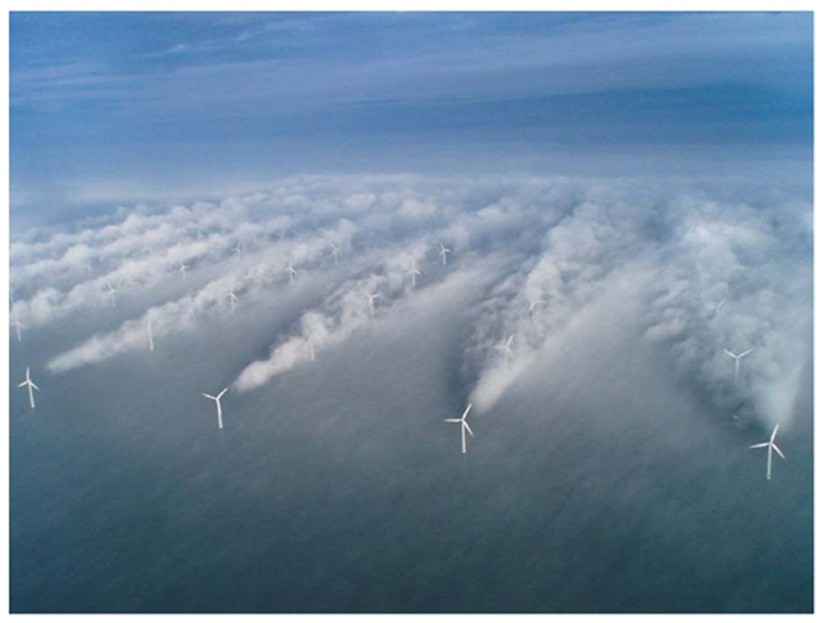
One of the main causes is the increasingly unequal and unbalanced fatigue loads in the OWFs, which are caused by the wake effect from using a conventional wind farm control. As Figure A1 in the section of Appendix A shows an image taken in February 2018 showing the obvious wake effects marked by humid air condensation in the Horns Rev OWF, Denmark. In material science theory, fatigue occurs when a material is subjected to repeated loading and unloading. In an OWF, the main causes of fatigue are the cyclic wind and wake disturbance loading and unloading, which affect the entire wind turbine structure. Based on the “Germanischer Lloyd” (GL) standard, Marín et al. [8] did research on the causes behind often-occurring failures. Sørensen et al. [9] analyzed the design code model based on probability theory and studied several fatigue models. Under wind loads, Barle [10] investigated the service strength. Under a maximum monotonic load, the static strength and fatigue were evaluated. Marino [11] considered different wind conditions, studied the fatigue loads and coupled response of a wind turbine. Wilkie et al. [12] investigated different environmental conditions, and built fatigue damage models based on Gaussian process regression.

As a relatively new technology, wind turbine control can improve wind turbine performance under operation and maintenance constraints [13]. Leithead et al. [14] studied active control approaches to cut the fatigue loads on a WT. Leithead et al. [15] proposed a control model to improve the performance of a WT. To reduce the effects of wind flow disturbance to WTs, Camblong [16] studied a control algorithm. Lescher et al. [17] investigated the linear parameter varying model of a WT, then designed a controller for multi-variable gain dispatching. To cut the maintenance cost of WTs, Sarker et al. [18] used preventive maintenance strategy, and proposed a maintenance cost model for offshore WTs. Based on Monte Carlo simulations, Ziegler et al. [19] studied a fatigue estimation model for monopile foundation of a WT. To reduce the structural loads on a WT, thereby prolonging its service life, Jackson et al. [20] designed a scheme using a new control strategy. To minimize the fatigue differences of WTs in a wind farm, Yao [21] optimized a power-dispatching model. To reduce the effect from wind-wave misalignment to the fatigue of WTs, Sun [22] proposed a pendulum-tuned mass damper in a 3D space. The present research on control algorithms and technologies above is effective for power dispatching and fatigue loads reduction for WTs. Wilkie [12] proposed that a WT control system should capture maximum wind energy, and extend the lifetime of the turbine’s components. From the perspective of wind farm operations, a high-efficiency control technology should mitigate the increasingly unbalanced fatigue loads on WTs in an OWF.

This study is organized as follows. In Section 2, we describe a general wind farm layout model and analyze the conventional power control approach used in OWFs. In Section 3, we introduce wind turbine fatigue, focusing on the wake effect as the main cause of the unequal turbine fatigue distribution in a OWF; establish a wind power mechanics in the far wake effect; and then improve the conventional fatigue definition into an integrated definition based on three factors: the mean wind force, wind turbulence, and power generation. We use automata theory to design a specific WFMC control topology in Section 4. 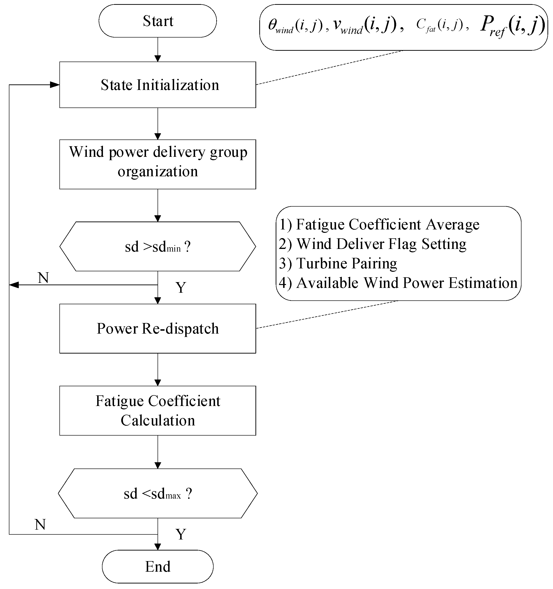In Section 5, the workflow of this novel power control approach is sketched. Section 6 presents the simulated results of this novel power control approach using wind energy data sampled in Horns Rev OWF. Section 7 discusses the performance of the conventional control approach and the improved control approach considering three important parameters: the mean turbine fatigue, the standard deviation (SD) of turbine fatigue, and the possible power loss. Finally, some important conclusions are drawn in Section 8.

2. Conventional Power Control in an OWF

2.1. OWF Layout Model

Without loss generality, we consider an array-geometry OWF with equidistant spacing between WT rows and lines, as shown in Figure 1. In an OWF, the distance between two neighboring turbines is about 5–8 rotor diameters, which can be considered far enough [23,24,25]. Assume that an OWF consists of m rows and n columns of WTs. Each wind turbine is marked with $T(i,j)$. The indices i varies from 1 to m, and j varies from 1 to n.

The wind speed measured by anemometers installed in each wind turbine decreases along the downstream direction. The studies in [26,27,28,29,30,31] estimated the wind speed reduction in an OWF. As an example, in the present work we used the wind data of the Horns Rev OWF, which is located at a reef approximately 14 km off Jutland in the North Sea in Denmark. The Horns Rev wind farm was built by the Danish Energy company Elsam (now DONG Energy) in 2002 and was the first OWF in the North Sea. This wind farm consists of 80 wind turbines (Vestas V80, nominal power 2.0 MW), with a total capacity of 160 MW and an annual power production of 600 MkWh [32].

2.2. Conventional Wind Farm Control

As described in [32], a Wind Farm Main Controller (WFMC) was designed and installed in the Horns Rev OWF. The WFMC acquires the wind data surrounding turbines and the electric power data from the transformer station, and, after power dispatching calculation, returns control signals to the turbines. To control the active power, the WFMC includes control functions such as: (a) the absolute production limiter, (b) the balance control, (c) the gradient limitation, and (d) the delta control. To control the reactive power, the WFMC includes the functions of a fixed MVA (i.e. Mega Volt Ampere) exchange and voltage control on the output from the transformer linked to the onshore grid. The communication to and from the WFMC between the SCADA (supervisory control and data acquisition) and the wind turbines is shown in Figure 2.

To date, most endeavors have sought to improve the electric power control for electricity requirements matching the grid. For example, the balance control function is implemented to meet the grid power requirements [32]. In [33], the power control laws were validated in an OWF. In [34], Condition Monitoring Systems were introduced to improve maintenance management and increase the reliability of OWFs. In fact, the loads on turbines cannot be balanced by a conventional WFMC approach, so turbine fatigue distribution cannot be balanced further for WT lifetime extending.

An advanced WFMC should consider both output power maximization and lifetime of the turbine components, such as the gearbox, the blades, and the tower [13]. One of the most popular approaches is to balance the natural wind load to the individual wind turbines, relying on a reasonable wind power dispatch approach, thereby equalizing turbine fatigue.

3. Improved Turbine Fatigue Definition

OWF control technology can provide opportunities to improve the performance of both WTs and wind farms under operation and maintenance limitations. In order to extend the lifetime of turbine components and thereby reduce the maintenance costs incurred by using boats or helicopters, the conventional control can be improved with considerations of both power generation and turbine fatigue balance. We study this control improvement based on precise and empirical wind power delivery models as follows.

3.1. Wind Power Mechanics with a Wake Effect

In order to analyze wind power delivery mechanics, some concepts are introduced from Betz’s Momentum [35].

3.1.1. Upstream Wind Power

In an offshore wind farm, the upstream wind power of the WT marked as $T(i,j)$, can be calculated as

$$P_{fro}(i,j)=\frac{1}{2}\rho v_{i,j}^{3}A$$

(1)

where $\rho$ is the air density, $v_{i,j}$ is the upstream wind speed, and A is the blade sweeping area. Then, the upstream wind power of wind turbine T(i+1, j) is

$$P_{fro}(i+1,j)=\frac{1}{2}\rho v_{i+1,j}^{3}A$$

(2)

in the case of a large OWF, in which most internal wind turbines are running in the downstream wake from front WTs. In order to estimate the wind power deficit caused by wind wake effects at any downstream distance, many wake models were developed, such as the Frandsen model, the Schlichting model, and the Jensen model [26].

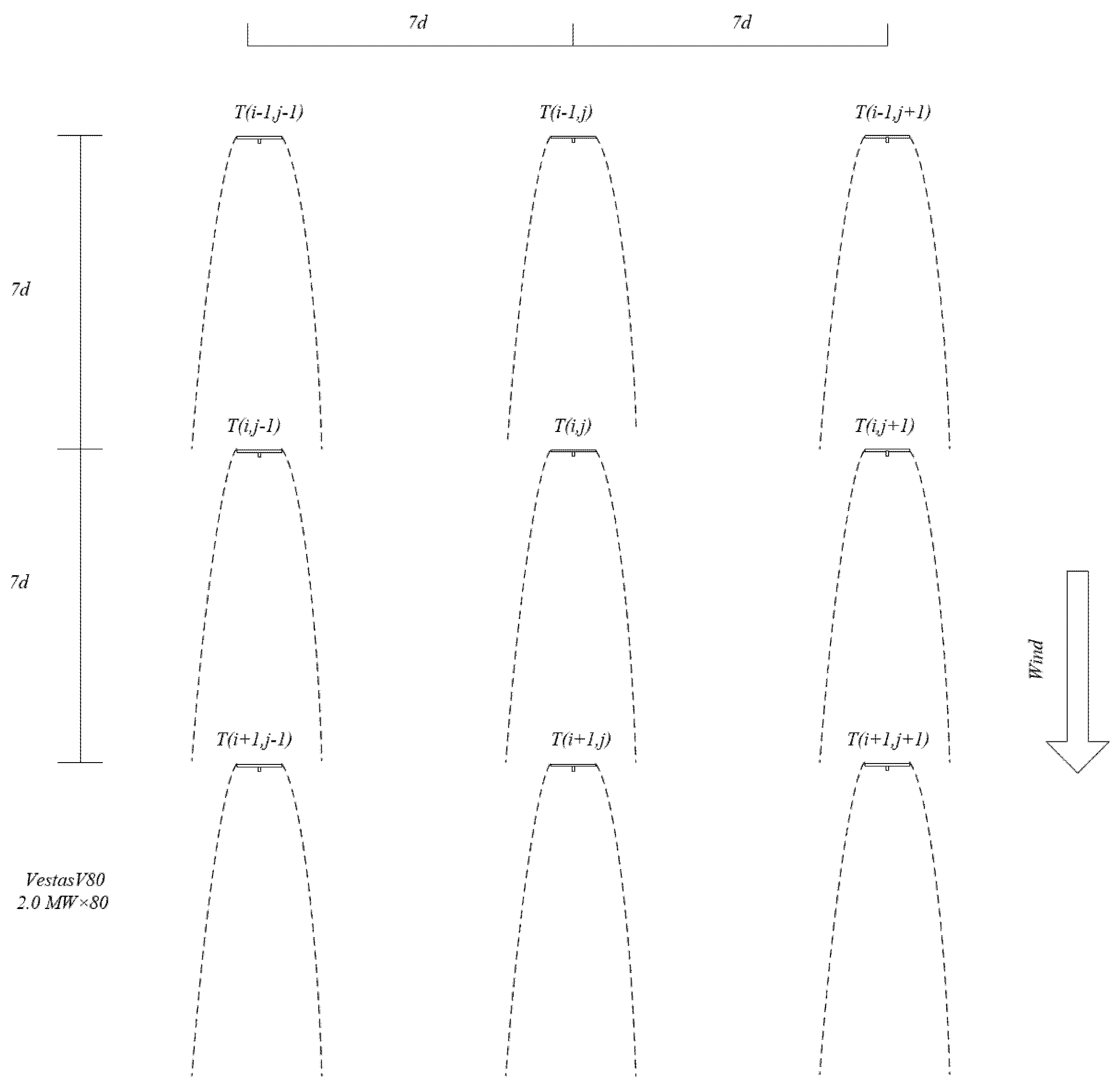
We assume that wind turbine $T(i+1,j)$ is located downstream from wind turbine $T(i,j)$ as shown in Figure 3. Here, the averaged ratio of the upstream wind speed of $T(i,j)$ to the upstream wind speed of $T(i+1,j)$ can be evaluated in (3). The distance between $T(i,j)$ and $T(i+1,j)$ is 7 rotor diameters (i.e., 7d), used in the Horns Rev OWF. The wind speed in this OWF varies from 2 to 24 m/s.

$$\frac{v_{i,j}}{v_{i+1,j}}=1.0767$$

(3)

This ratio is approximately equal to the value mentioned in [23] based on the engineering experience of velocity deficits in the far wake of an OWF.

3.1.2. Wind Power Delivery

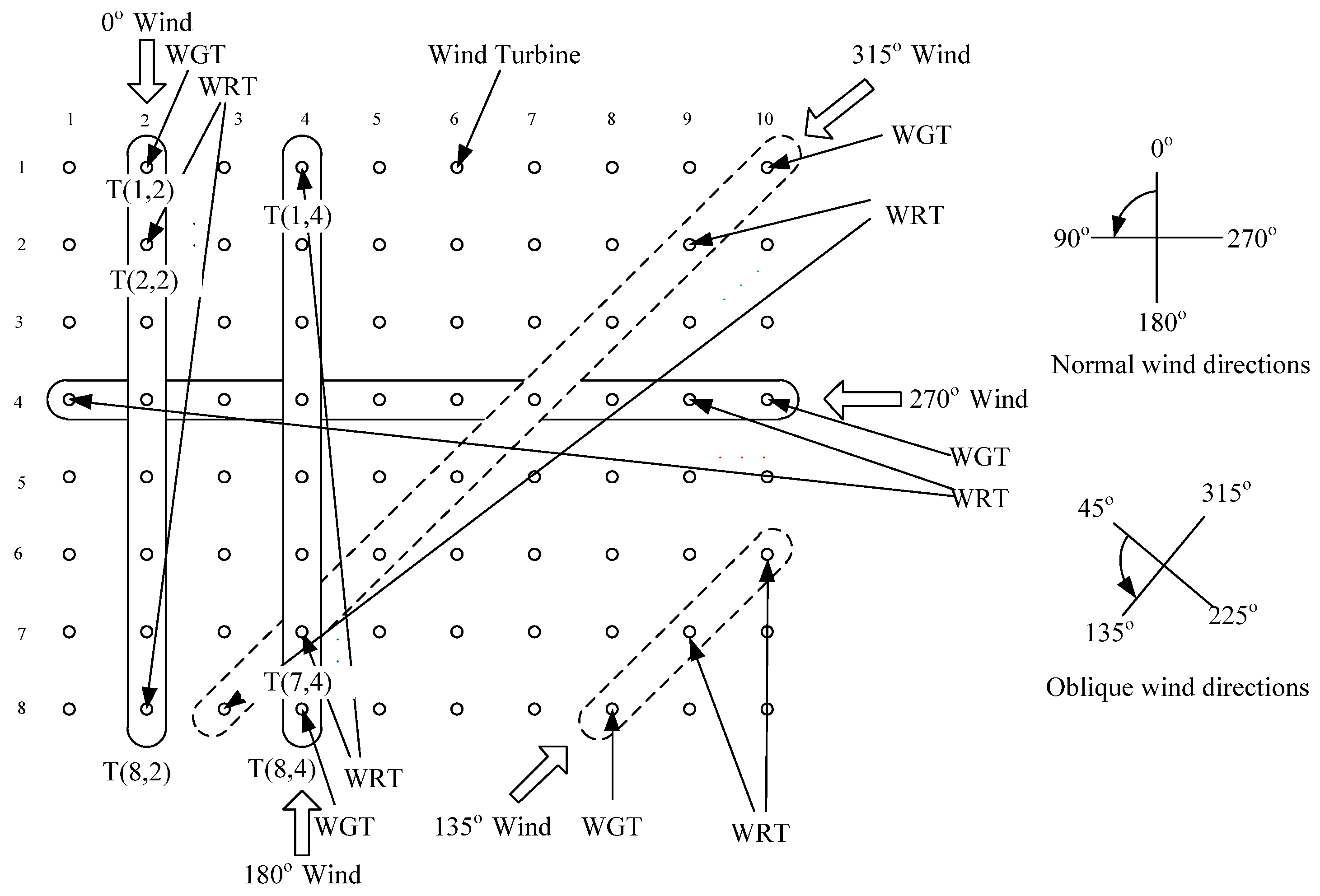
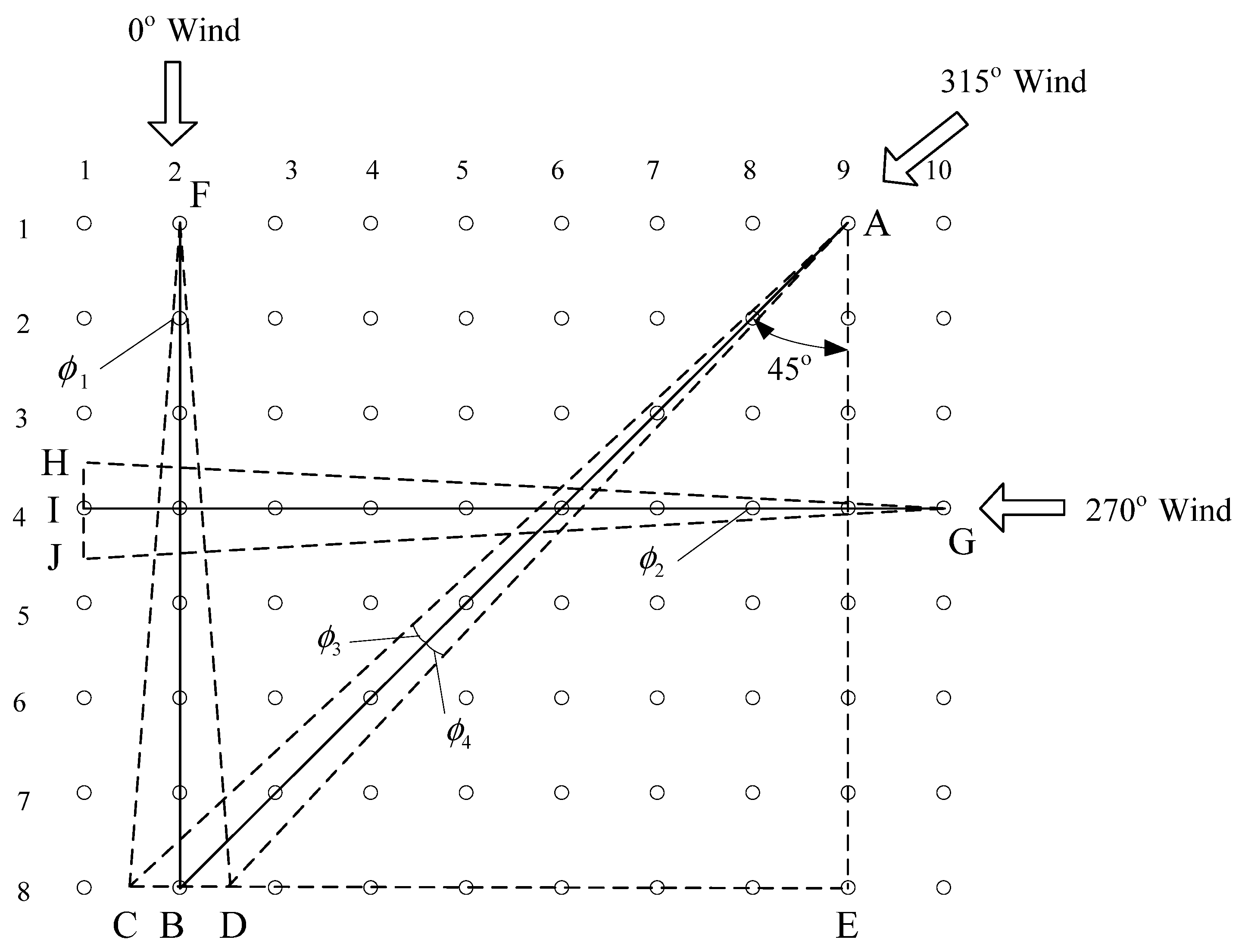
Based on the observed wind data acquired from the Horns Rev OWF in references [23,35], the coefficient wind power delivery is defined as the ratio of the decreased power of the upstream turbine to the increased power of its downstream partner during wind power delivery. In order to simplify the wind direction category, this study focuses on two main wind direction categories, normal power delivery and oblique power delivery, as shown in Figure 4. In the case of normal power delivery, the wind directions are normal to the WT rows or columns. The main wind angles are 0°, 90°, 180°, and 270°. The corresponding wind power delivery group has a solid line boundary in Figure 4. In the case of oblique power delivery, the wind direction is oblique to the wind farm layout. The wind angles considered here are 45°, 135°, 225°, and 315°. The corresponding wind power delivery group is marked with dashed line bars in Figure 4.

• Category 1. Normal power delivery

We assume that a downstream turbine only absorbs some part of the wind energy after the energy absorption from the upstream turbines in the same column along the downstream direction. The initial upstream wind speed of the first turbine is 8 ± 0.5 m/s¹. As wind moves through the wind farm downstream, the wake widths considered are ±1° and ±5°.

Case 1, wind direction 0° or 180°:

For a single column along the wind direction, the normalized power ratios between the second turbine to the first turbine and subsequent turbines to their front turbines are

$${\alpha }_{(0^0\pm 1^0,2-1,\mathrm{j})}=\frac{P_{fro}(2,j)}{P_{fro}(1,j)}=\frac{0.621}{1.000}=0.621$$

(4)

$${\alpha }_{(0^0\pm 1^0,3-2,\mathrm{j})}=\frac{P_{fro}(3,j)}{P_{fro}(2,j)}=\frac{0.629}{0.621}=1.013$$

(5)

$${\alpha }_{(0^0\pm 1^0,4-3,\mathrm{j})}=\frac{P_{fro}(4,j)}{P_{fro}(3,j)}=\frac{0.601}{0.629}=0.956$$

(6)

$${\alpha }_{(0^0\pm 1^0,5-4,\mathrm{j})}=\frac{P_{fro}(5,j)}{P_{fro}(4,j)}=\frac{0.602}{0.601}=1.002$$

(7)

$${\alpha }_{(0^0\pm 1^0,6-5,\mathrm{j})}=\frac{P_{fro}(6,j)}{P_{fro}(5,j)}=\frac{0.603}{0.602}=1.002$$

(8)

$${\alpha }_{(0^0\pm 1^0,7-6,\mathrm{j})}=\frac{P_{fro}(7,j)}{P_{fro}(6,j)}=\frac{0.607}{0.603}=1.007$$

(9)

$${\alpha }_{(0^0\pm 1^0,8-7,\mathrm{j})}=\frac{P_{fro}(8,j)}{P_{fro}(7,j)}=\frac{0.610}{0.607}=1.004$$

(10)

With a 180° wind direction, the power ratio sequence is inverted (i.e., (1.004,1.007,1.002,1.002,0.956,1.1013,0.621)). According to Reference [23], this analysis focuses on the wake center areas, where the wind power at the second WT and subsequent WTs is approximately 60% freestream [23].

Case 2, wind direction 90° or 270°:

With a 90° or 270° wind direction, the normalized power ratios between the second turbine, the first turbine, and subsequent turbines to their front turbines are approximately the same as the values in case 1. The only difference is that the turbine number in a single row is ten in case 2. The wind power at the second WT and subsequent WTs is approximately 60% freestream [23].

When an upstream turbine $T(i,j)$ is more fatigued than a downstream turbine, we can control its pitch angle to absorb less wind power; therefore, an additional portion of the wind power will be delivered to the downstream wind turbine. This additional wind power, denoted as $\Delta P_{fro}(i+k,j)$, will be absorbed by the downstream turbine if the wind flow falls in the range of the cut-in speed and the rated speed. The partial-load conditions and wind power increment can be calculated as

$$\Delta P_{fro}\left(i+k,j\right)={\displaystyle \prod }_k^{n-1}{\alpha }_{\left(\mathrm{i}+\mathrm{k}+1\right)-\left(\mathrm{i}+\mathrm{l}\right)}^k\Delta P_{fro}\left(i,j\right)$$

(11)

In partial-power conditions (which a wind turbine most commonly runs in), $c_p$ is considered as a constant. In full-power conditions, $c_p$ is assumed to be piecewise linear [4]. Thus, we can evaluate the electric power change as

$$\Delta P(i,j)=c_p|\Delta P_{fro}(i,j)|$$

(12)

Further, based on Equations (10) and (11),

$$\Delta P\left(i+k,j\right)=c_p\left|{\displaystyle \prod }_k^{n-1}{\alpha }_{\left(\mathrm{i}+\mathrm{k}+1\right)-\left(\mathrm{i}+\mathrm{l}\right)}^k\Delta P_{fro}\left(i,j\right)\right|$$

(13)

If the electric power change ΔP(i,j) is due to the change of the pitch angle, rather than a change of wind speed, we expect that the upstream turbine T(i,j) leaves some of its front wind power to its downstream partner, the turbine agent $T(i+k,j)$. Then,

$$\Delta P(i,j)<0\Rightarrow \Delta P(i+k,j)>0$$

(14)

In the sections below, for simplicity, we assume all $\Delta P(i,j)$ to be positive.

• Category 2. Oblique power delivery

When the wind blows obliquely to the wind farm, we consider the main directions of 45°, 135°, 225°, and 315° shown in Figure 4. The distance between the neighboring upstream and downstream turbines along one of the aforementioned oblique directions is $x=7\sqrt{2}d$. For a single column along the wind directions of 45°, 135°, 225°, and 315° (the same power ratios as the wind direction of 312°; case 3 in [23]), the normalized power ratios of the second turbine to the first turbine and of subsequent turbines to their front turbines are

$${\alpha }_{({45}^0\pm 1^0,2-1,2-1)}=\frac{P_{fro}(2,2)}{P_{fro}(1,1)}=\frac{0.858}{1.000}=0.858$$

(15)

$${\alpha }_{({45}^0\pm 1^0,3-2,3-2)}=\frac{P_{fro}(3,3)}{P_{fro}(2,2)}=\frac{0.801}{0.858}=0.934$$

(16)

$${\alpha }_{({45}^0\pm 1^0,4-3,4-3)}=\frac{P_{fro}(4,4)}{P_{fro}(3,3)}=\frac{0.758}{0.801}=0.946$$

(17)

$${\alpha }_{({45}^0\pm 1^0,5-4,5-4)}=\frac{P_{fro}(5,5)}{P_{fro}(4,4)}=\frac{0.703}{0.758}=0.927$$

(18)

$${\alpha }_{({45}^0\pm 1^0,6-5,6-5)}=\frac{P_{fro}(6,6)}{P_{fro}(5,5)}=\frac{0.689}{0.703}=0.980$$

(19)

$${\alpha }_{({45}^0\pm 1^0,7-6,7-6)}=\frac{P_{fro}(7,7)}{P_{fro}(6,6)}=\frac{0.668}{0.689}=0.969$$

(20)

$${\alpha }_{({45}^0\pm 1^0,8-7,8-7)}=\frac{P_{fro}(8,8)}{P_{fro}(7,7)}=\frac{0.659}{0.668}=0.987$$

(21)

The wind power of WT can be calculated as

$$P_{fro}\left(i+k,j+k\right)={\displaystyle \prod }_k^{n-1}{\alpha }_{\left(\mathrm{i}+\mathrm{k}+1\right)-\left(\mathrm{i}+\mathrm{l}\right),\left(\mathrm{i}+\mathrm{k}+1\right)-\left(\mathrm{i}+\mathrm{l}\right)}{P}_{fro}\left(i,j\right)$$

(22)

where k varies from 1 to m-i. When an upstream turbine delivers partial wind power, to its oblique downstream partner, the delivery power is

$$\Delta P_{fro}\left(i+k,j+k\right)={\displaystyle \prod }_k^{n-1}{\alpha }_{\left(\mathrm{i}+\mathrm{k}+1\right)-\left(\mathrm{i}+\mathrm{l}\right),\left(\mathrm{i}+\mathrm{k}+1\right)-\left(\mathrm{i}+\mathrm{l}\right)}\Delta P_{fro}\left(i,j\right)$$

(23)

The electric power change relationship between wind turbines $T(i,j)$ and $T(i+k,j+k)$ is

$$\Delta P\left(i+k,j+k\right)={\displaystyle \prod }_k^{n-1}{\alpha }_{\left(\mathrm{i}+\mathrm{k}+1\right)-\left(\mathrm{i}+\mathrm{l}\right),\left(\mathrm{i}+\mathrm{k}+1\right)-\left(\mathrm{i}+\mathrm{l}\right)}\Delta P\left(i,j\right)$$

(24)

Note that the two delivery coefficients ${\alpha }_N$ and ${\alpha }_o$ above are theoretical parameters for ideal large OWFs. They can be adjusted according to real wind conditions and wind farm layouts.

3.2. Conventional Fatigue Definition

The WT fatigue is a very complex technical issue. In the material area, in the case of cyclic loading or loading and unloading, fatigue is the progressive damage. Here, we introduce two conventional fatigue definitions.

• Definition 1. Power fatigue

In general, a turbine is fatigue-loaded and then generates electric power. The work in [36] counted all the electric power from a WT’s installation and defined the power fatigue coefficient as

$$C_{fatigue}=\frac{{\displaystyle \underset{0}{\overset{t_0}{\int }}p(t)dt}}{P_{rated}{T}_{lifetime}}$$

(25)

where $t_0$ is the working duration from the wind turbine installation, $P_{rated}$ is the WT’s rated power, and $T_{lifetime}$ is the whole designed WT lifetime (e.g., 25 years).

• Definition 2. Equivalent fatigue loads

The turbulence intensity increases significantly in the wake regions of OWFs. According to [37,38,39,40], the main fatigue factor is, as expected, the turbulence intensity.

Considering that the ratio of the standard deviations of turbulence in the axial velocity to the wind speed at the hub is 0.15, without yaw errors. The equivalent loads $L_{eq}$ is

$$L_{eq}={({\displaystyle \sum _i{L}_i^m{n}_i/N_{eq}})}^{1/m}$$

(26)

where $1/m$ is the material S–N curve slope. $N_{eq}$ is the total number of rotations.

Analyzing the two fatigue definitions above reveals some difficulties. First definition 1 (power fatigue) only counts electric power generation while neglecting the wind turbulence loads to the different turbine parts, such as the rotor, the blades, the gearbox, and the tower. Second, definition 2 (equivalent fatigue loads) can calculate the turbulence in the form of load cycles, while the equivalent cycle cannot be calculated with the turbine rotation period in real operation.

3.3. Improved Fatigue Definition

To balance the WT fatigue distribution in an OWF, an improved fatigue can be defined considering both the electric power generation and the real wind turbulence intensity.

In real wind farm operations, the individual wind turbine always suffers basic mean wind loads and cyclic wind turbulence loads, even when the turbine is at a standstill. However, the more electric power a turbine generates, the more turbulence loads it will suffer alongside stronger mean wind force on the turbine’s structure. Therefore, we consider the mean wind loads, the cyclic wind turbulence loads, and the power generation loads to define an easily calculated fatigue coefficient.

In this study, we consider the rated power, generated power, wind turbulence, and service life of a WT. Here, WT installation moment $\mathrm{t}=0$ and the present moment $\mathrm{t}=t_p$. Considering the factors above, we define the improved fatigue coefficient as

$$C_{fat}=f_{mean}+f_{tur}+f_{work}=C_{mean}\frac{{\displaystyle {\int }_0^{t_p}{I}_{mean}(t)dt}}{T_{ser}(1+p_{rep})}+C_{tur}\frac{{\displaystyle {\int }_0^{t_p}{I}_{eff}(t)dt}}{T_{ser}(1+p_{rep})}+\frac{{\displaystyle {\int }_0^{t_p}p(t)dt}}{P_{rat}{T}_{ser}(1+p_{rep})}$$

(27)

where $C_{fat}$ is the improved fatigue coefficient of a WT including three factors:

• $f_{mean}$ is the fatigue caused by the mean cyclic wind flow, denoted as the mean wind fatigue. This mean wind varies slowly. The cyclic mean wind flow is the averaged wind speed measured by an anemometer installed on the nacelle. This mean wind flow acts on the wind turbine with a large force but a low frequency and thus causes a lower fatigue than the wind turbulence imposed by the wake disturbance.

$C_{mean}$ is the mean wind flow coefficient determined by the OWF layout, the WT’s material structure, and the surrounding wind flow conditions; $T_{ser}$ is the WT lifetime, and $p_{rep}$ is the recovery coefficient (0–1) after regular repair. In fact, the whole service life will be extended when some key components are repaired. $I_{mean}(t)$ is the mean wind load intensity, which has the same dimension as the wind power and can be calculated as

$$I_{mean}(t)={\beta }_{mean}v{(t)}_{i,j}^{3}A$$

(28)

where ${\beta }_{mean}$ is the mean wind load coefficient, determined by the local wind conditions and the specific structure of the turbine; ${v(t)}_{i,j}$ is the average wind speed measured by turbine anemometer; and A is the blade-sweeping area.

2.

$f_{tur}$ is fatigue caused by wind turbulence, mainly on the blades, the nacelle, and the tower, denoted as wind turbulence fatigue. $C_{tur}$ is the wind turbulence coefficient depending on the local climatic conditions, OWF layout, and WT material structure. To calculate, in Figure 4 of [41], the measured turbulence intensities in the overlapped-wake sections can be used; $I_{eff}(t)$ is the turbulence intensity. In [41], the ambient turbulence intensity $I_a(t)$ and the wake turbulence intensity contribution $I_w(t)$ can be used to evaluate turbulence intensity $I_{eff}(t)$ as:

$$I_{eff}(t)=\sqrt{I_a{(t)}^2+I_w{(t)}^2}$$

(29)

where, according to [41], $I_w(t)$ is calculated as

$$I_w(t)=\frac{1}{S}\sqrt{1.2C_t(t)}$$

(30)

where S is the distance between two WTs, $C_t(t)$ is the WT thrust coefficient.

3.

$f_{work}$ is the power generation fatigue. Here, $p(t)$ is the transient power at time t. $P_{rat}$ is the nominal power.

In order to make the technique applicable to different OWFs, an empirical compound ratio between the mean wind fatigue, turbulence fatigue, and work fatigue is proposed as follows:

$$\gamma =f_{mea}/f_{dis}/f_{work}$$

(31)

where $\gamma$ is determined according to site climate conditions, the OWF layout, and the WT structure.

Equation (26) can be improved in two cases as:

$$C_{fat}=\{\begin{array}{c}{C}_{fat}(t_0)+f_{mea}+f_{tur}+f_{work}\hspace{1em}\hspace{1em}\hspace{1em}if\hspace{0.17em}{v}_{cut-in}<v<\hspace{0.17em}{v}_{cut-off}\hspace{1em}\hspace{1em}\\ C_{fat}(t_0)+f_{mea}+f_{tur}\hspace{1em}\hspace{0.17em}\hspace{0.17em}\hspace{1em}\hspace{1em}\hspace{1em}\hspace{1em}if\hspace{0.17em}\hspace{0.17em}v<v_{cut-in}\hspace{0.17em}or\hspace{0.17em}v>v_{cut-off}\end{array}\hspace{1em}$$

(32)

where $C_{fat}(t_0)$ is the fatigue coefficient at time $t_0$. $f_{work}$ will be equal to zero when a wind turbine does not generate power, corresponding to situations when the wind speed lies outside the effective wind speed range ($v_{cut-in},v_{cut-off}$) or the turbine is braked for maintenance.

4. WFMC Control Topology

Based on the above, this improved fatigue coefficient can be used as the basic parameter to evaluate the fatigue status of individual WTs in an OWF. The wind farm’s operational and maintenance costs can be reduced if the lifetime of the wind turbines can be extended using an effective fatigue control approach. Likewise, the frequency of maintenance using boats and helicopters can be reduced. Considering the fatigue improvement, we construct a control topology for a WFMC based on automata theory.

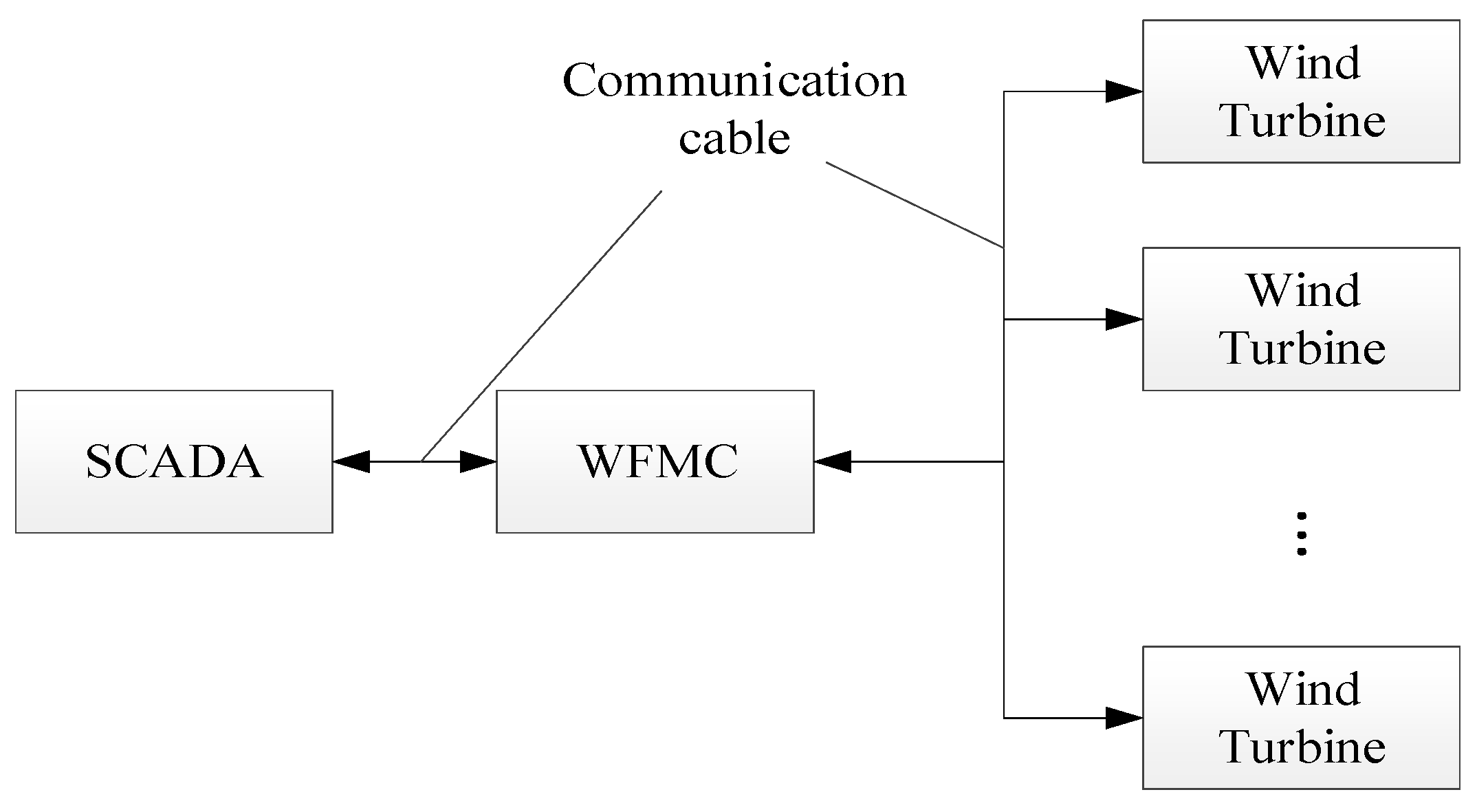
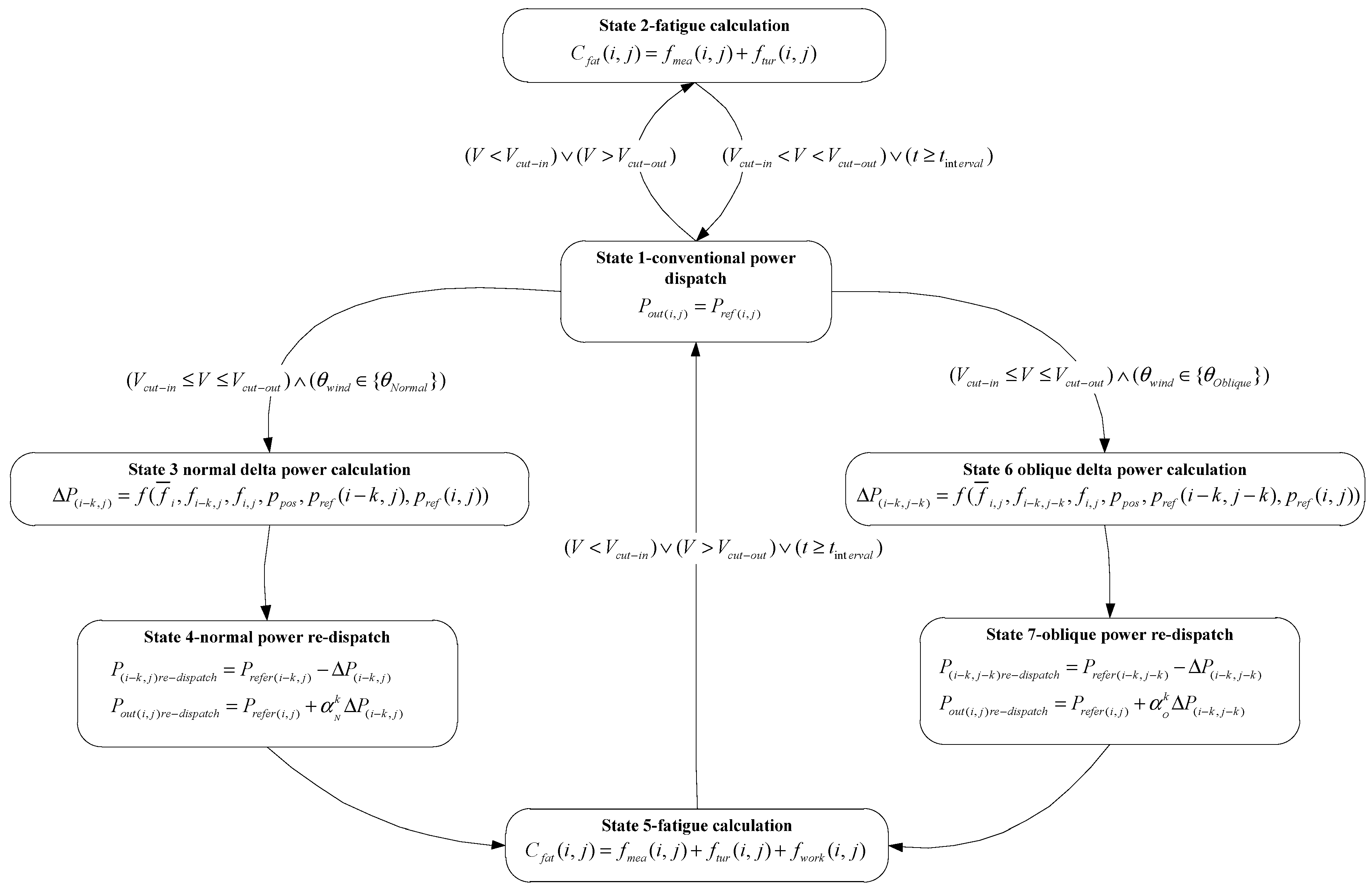
Based on the data from individual turbines and the measured data from the transformer station in [32], the WFMC returns control signals to the WTs. In order to regulate the active power, the WFMC implements the control functions including Absolute Production Limiter, Balance Control, Gradient Limitation, Delta Control, and Reactive Power Control. Besides these typical functions, we propose a fatigue-optimization-based control topology for a WFMC as shown in Figure 5.

This fatigue-based control topology consists of seven operational states that the WFMC can possibly run in. State 1 is a conventional power dispatch state, which is the current work state of the WFMC. The equation $P_{out(i,j)}=P_{ref(i,j)}$ indicates that the WFMC dispatches the reference power to the individual turbines according to the data of the individual WTs and the measured power data from the transformer station. Therefore the output power of each wind turbine, denoted as $P_{out(i,j)}$, is equal to the reference power, denoted as $P_{ref(i,j)}$.

State 2 is the fatigue calculation. The WFMC will run in state 2 when the guard $(V<V_{cut-in})\vee (V>V_{cut-out})$ is met. In state 2, the main work of the WFMC is to calculate the fatigue without counting power fatigue, i.e.,$f_{work}=0$. Conversely, the WFMC will return to state 1 when the guard is enabled, which means that the wind speed is in the range of the cut-in speed and the cut-out speed or that the calculation interval (e.g., 30 minutes) is over. In State 2, the main work is to calculate the fatigue without counting power fatigue, i.e., $f_{work}=0$.

State 3 entails normal delta power calculation. The WFMC will operate in state 3 when the guard $(V_{cut-in}\le V\le V_{cut-out})\wedge ({\theta }_{wind}\in \{{\theta }_{Normal}\})$ is enabled, and the wind direction falls in the range of the permitted angle tolerance around the main normal wind directions, e.g., 0°, 90°, 180°, and 270°. In state 3, as equation $\Delta P_{(i-k,j)}=f({\overline{f}}_i,f_{i-k,j},f_{i,j},p_{pos},p_{ref}(i-k,j),p_{ref}(i,j))$ shows, the main work of the WFMC is to calculate the delta power for each WT according to the average fatigue of the WTs in the same column along a normal wind direction, the fatigue values of WTs to be paired, the possible power output, and the reference power values of the turbines; the WFMC will then move directly into state 4, the normal power re-dispatch, when the normal delta power calculation is finished in state 3.

State 4 is the normal power re-dispatch. In state 4, as equations $P_{(i-k,j)re-dispatch}=P_{refer(i-k,j)}-\Delta P_{(i-k,j)}$ and $P_{out(i,j)re-dispatch}=P_{refer(i,j)}+{\alpha }_N^{-k}\Delta P_{(i-k,j)}$ show in Figure 5, the main function of the WFMC is to re-dispatch the power for each wind turbine, according to the results from state 3, to balance the turbulence load on the WTs in a wind farm. The WFMC will move directly into state 5, fatigue calculation, when the power re-dispatch is finished in state 4.

State 5 involves fatigue calculation. In state 5, as the equation $C_{fat}(i,j)=f_{mea}(i,j)+f_{tur}(i,j)+f_{work}(i,j)$ shows in Figure 5, the main work of the WFMC is to calculate the fatigue coefficient for each wind turbine based on the mean wind fatigue $f_{mea}(i,j)$, the wind turbulence fatigue $f_{work}(i,j)$, and the work fatigue in every wind power dispatch interval. The WFMC will return directly into state 1, the conventional power dispatch, when the guard $(V<V_{cut-in})\vee (V>V_{cut-out})\vee (t\ge t_{\mathrm{int}erval})$ is enabled.

State 6 entails the oblique delta power calculations. The WFMC will operate in state 6 when the guard $(V_{cut-in}\le V\le V_{cut-out})\wedge ({\theta }_{wind}\in \{{\theta }_{Oblique}\})$ is enabled, which means that the wind speed is in the range of the cut-in speed and the cut-out speed, and the wind direction falls in the range of the permitted angle tolerance around the main oblique wind directions, e.g., 45°, 135°, 225°, and 315°. In state 6, the main work of the WFMC is to determine the delta power for each WT along the oblique directions; the WFMC will then move directly into state 7, the oblique power re-dispatch, when the normal delta power calculation is finished in state 6.

State 7 is the oblique power re-dispatch. In state 7, the WFMC re-dispatches the power for each WT along the oblique directions, according to the results from state 6. The WFMC will move directly into state 5, the fatigue calculation, when the oblique power re-dispatch is finished in state 7.

In addition, in states 3 and 6, $\Delta P$ is the delivery power determined in the WFMC. $\Delta P$ is empirically as

$$\Delta P=\{\begin{array}{c}2(P_{ref}-\overline{P_{kk}}),\hspace{0.17em}if\hspace{0.17em}{P}_{ref}-2(P_{ref}-\overline{P_{kk}})\hspace{0.17em}>0\\ 0.8P_{ref},otherwise\hspace{1em}\hspace{1em}\hspace{1em}\hspace{1em}\hspace{1em}\hspace{1em}\hspace{1em}\hspace{1em}\end{array}$$

(33)

where $\overline{P_{kk}}$ is the mean power value in the power delivery group No.$\mathrm{kk}$.

5. Workflow of the Wind Farm Main Controller

We design the WFMC workflow in Figure 6 according to topology above.

5.1. Workflow of the WFMC

In the organization process of wind power delivery group, the WFMC organize all the turbines in the normal or oblique directions into parallel groups. Then, the WFMC will judge whether the SD of the WT fatigue distribution is larger than the minimum value, i.e., “sd > sd_min?” or not. If the result is true, the WFMC moves into the power re-dispatch process; otherwise, the WFMC returns to its initialization state.

Sequentially, the WFMC calculates the mean fatigue of each organized group, compares each turbine fatigue coefficient with the group averaged value, $\overline{c_{\mathrm{Group}}}$, and establishes flags to represent which turbine(s) need to cut their power output because of their over-loaded fatigue and which turbine(s) can absorb more wind power because of their under-loaded fatigue. Based on the fatigue, the power delivery turbine pairs are organized in such a way that the WT with the most fatigue pairs with the WT with the least fatigue, the second most fatigued pairs with the second least fatigued one, etc. According to the wind power mechanics with a wake effect in Section 3, the re-dispatched power output of the OWF is theoretically less than the dispatched power because of the wind speed deficit in the wake area, while the wind turbine fatigue can be equalized gradually with this improved power control approach. This is the primary novelty in the improved fatigue definition, WFMC control topology, and workflow presented in this study.

5.2. Wind Direction Tolerance

In order to apply theoretical models into a natural wind farm, the permitted tolerance around the main angles (i.e., the normal angles and oblique angles) should be considered.

Angle tolerances are usually defined as the angle varying range. For example, the minimum permitted tolerance of the Horns Rev OWF (see Figure 7) for 315° wind can be calculated by triangle geometry. Permitted angles (from ${\varphi }_1$ to ${\varphi }_4$) are calculated as

$${\varphi }_1={\tan }^{-1}(\frac{CB}{FB})={\tan }^{-1}(\frac{0.5\times 7d}{7\times 7D})=4.0856°$$

(34)

$${\varphi }_2={\tan }^{-1}(\frac{HI}{IG})={\tan }^{-1}(\frac{0.5\times 7d}{9\times 7D})=3.1798°$$

(35)

$${\varphi }_3={\tan }^{-1}(\frac{CE}{EA})-45°={\tan }^{-1}(\frac{0.5\times 7D+7\times 7D}{7\times 7D})-45=1.9749°$$

(36)

$${\varphi }_4=45°-{\tan }^{-1}(\frac{DE}{EA})=45°-{\tan }^{-1}(\frac{0.5\times 7D+6\times 7D}{7\times 7D})=2.1211°$$

(37)

In the oblique wind angle cases, we consider the minimum angles from ${\varphi }_3$ and ${\varphi }_4$ as

$$A_{tol}=\pm min\{{\varphi }_3,{\varphi }_4\}=\pm 1.9749°$$

(38)

Based on these calculations above, the tolerances of the wind direction angles of 0°, 45°, 90°, 135°, 180°, 225°, 270°, and 315° are calculated as

$$A_{tol}=\{\begin{array}{c}\pm 4.0856°,\hspace{0.17em}{\theta }_{wind}=0°, 180°\hspace{1em}\\ \pm 1.9749°,\hspace{0.17em}{\theta }_{wind}=45°, 135°, 225°\\ \pm 3.1798°,\hspace{0.17em}{\theta }_{wind}=90°, 270°\hspace{1em}\hspace{1em}\end{array},315°$$

(39)

where $\overline{C_{fat}}$ is the average of all turbine fatigue values, and $s{t}_{\min }$ is the minimum value of the calculated SD of $C_{fat}(i,j)$, which is set with a feasible constant, such as 0.0001, in this work.

6. Numerical Simulations

To validate this fatigue-based power control approach, we use the database of the Technical University of Denmark [38]. The resource data can be used for wind turbine design, wind farm sitting analysis, and operational optimization.

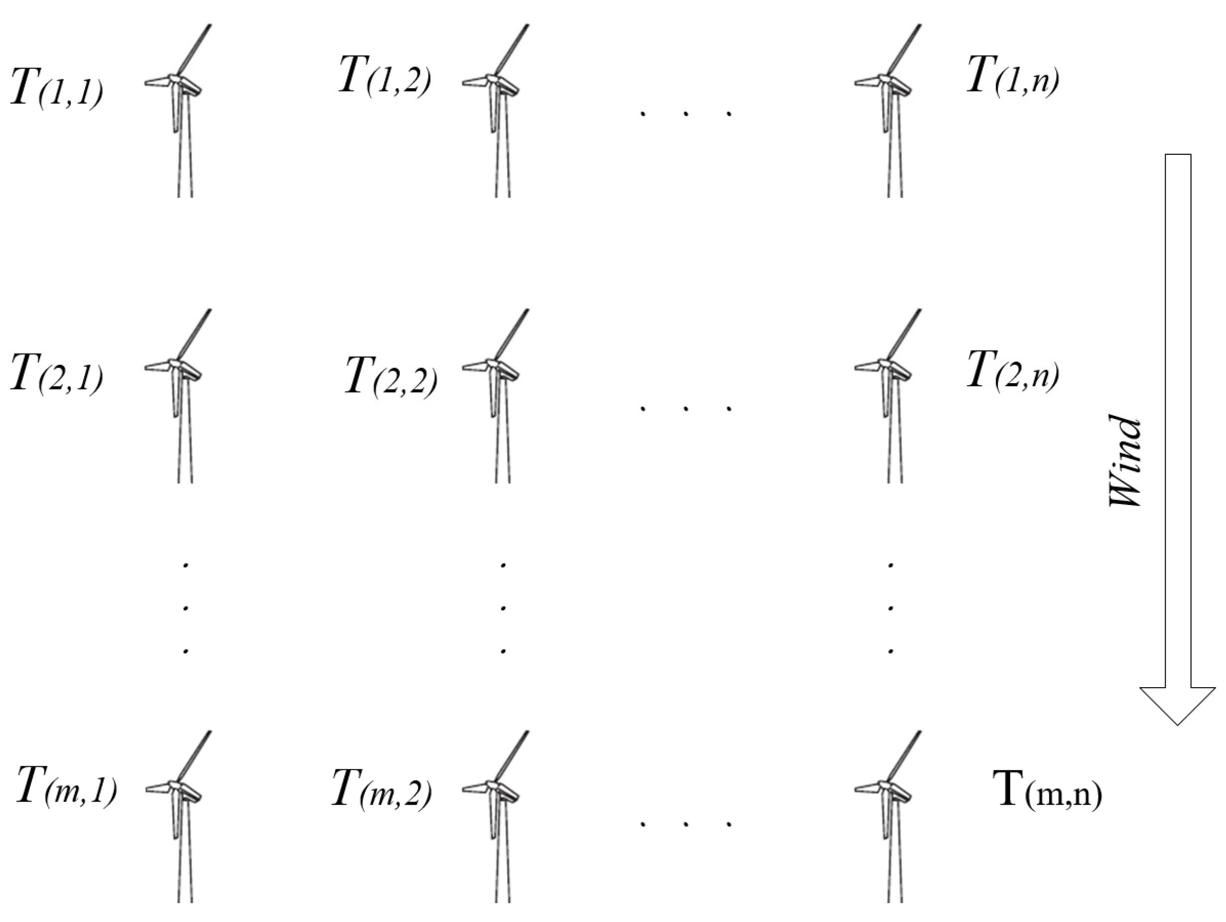
In this study, we use the Horns Rev OWF as an engineering example to test the wind farm model shown in Figure 1. The Horns Rev OWF is one of the largest OWFs in the world [38].

The natural wind condition is that the wind speed is 2–24 m/s, and the mean wind speed is 9.6 m/s at a 62 m hub height. The wind turbulence intensity falls in the range of 2% to 20%, and the mean value is 4.5206%. The wind direction falls in the range of 0° to 100°, and 270° to 360°.

We executed simulation code programmed in MATLAB 2019a [40]. Then, we imported the wind data and the basic power control parameters of the Horns Rev OWF into the simulation program and calculated the improved fatigue coefficient with this novel power control approach. Finally, the simulation results illustrate the farm fatigue distribution in both the conventional control approach and the improved control approach. The simulation parameters are listed as:

(a)

The mean wind speed value is 9.6 m/s with a turbulence intensity of 4.5206% as in [38].

(b)

The empirical compound ratio $\gamma =f_{mea}/f_{dis}/f_{work}=0.3/0.6/1.0$.

(c)

The data on wind directions was obtained from [38]. The main wind directions were 0°, 45°, 90°, and 315° with the tolerance values estimated in Equation (28).

(d)

Simulation stages: the conventional farm control approach was assumed for 8 years (from Dec., 2002 to Nov., 2010) and the improved control approach was assumed for another 8 years (from Dec., 2010 to Nov., 2018).

(e)

In the Horns Rev wind farm, considering the actual wind farm conditions where the wake effect tends to saturate after three turbines, in a power delivery group, we assume that an upstream turbine is able to deliver its power to one of three downstream turbines.

(f)

WFMC power dispatching interval is 30 mins.

(g)

The optimal target is to minimize the fatigue SD in the whole OWF below a threshold of 0.0001.

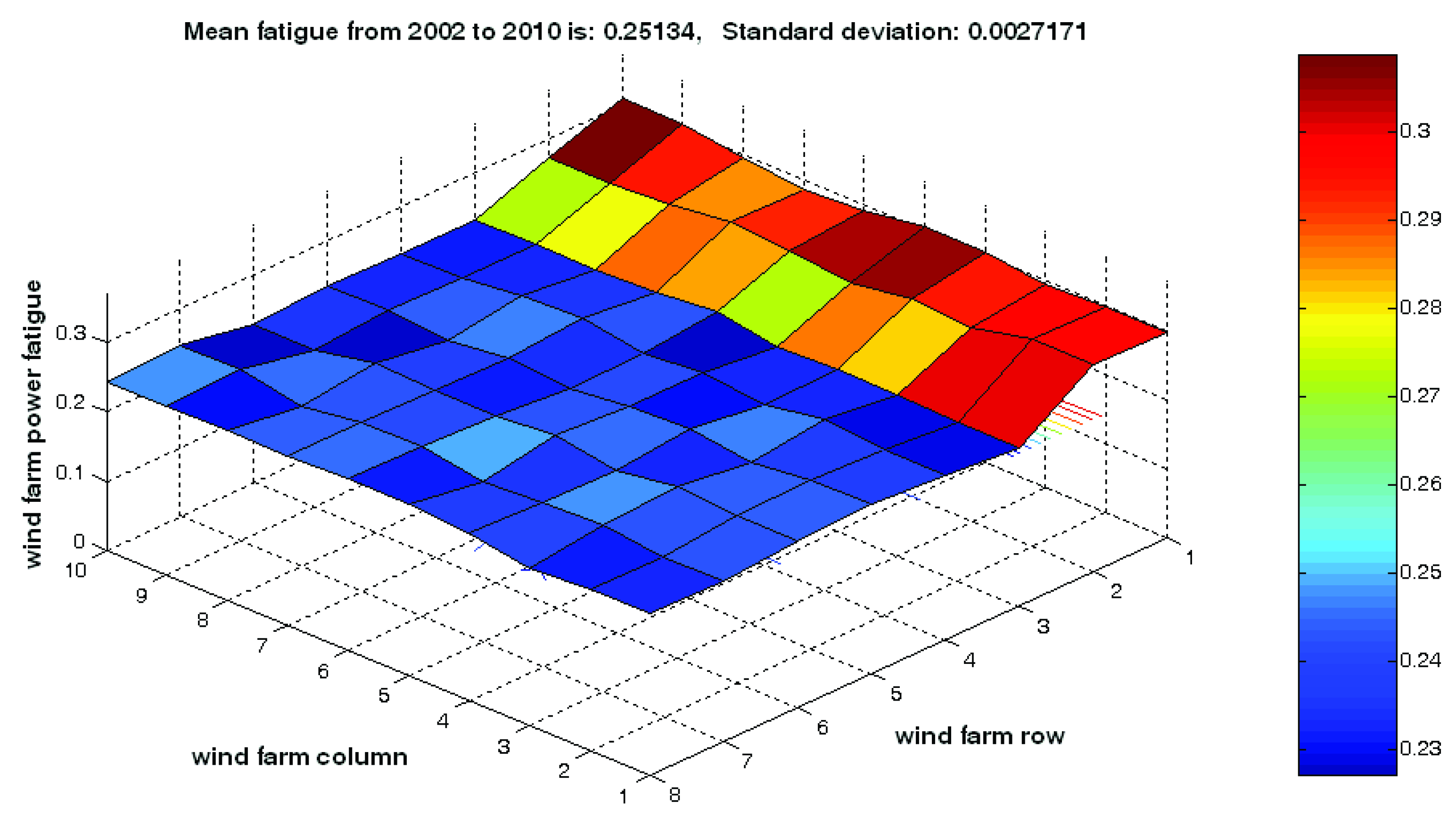
During the initial stage of the simulation, a zero fatigue distribution is configured according to the wind farm’s operation starting in December, 2002. Figure 8 shows WT fatigue distribution using the conventional control method [32] over the duration of 70,080 hours. Here, the turbine fatigue values are clearly unequal and irregularly distributed over the whole wind farm area.

For the duration of 2002-2010, as shown in Figure 8, the mean fatigue of all the turbines in this wind farm is 0.25134, and the SD of the turbine fatigue distribution is 0.0027171.

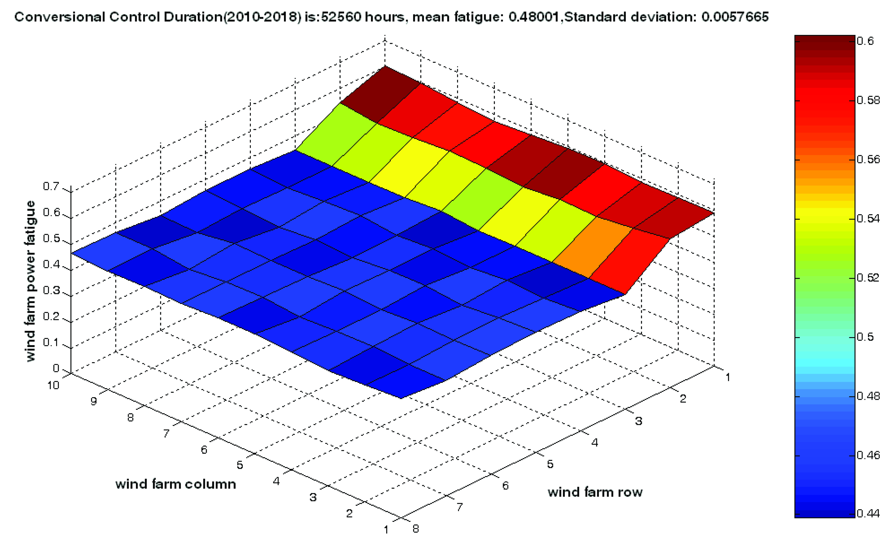
For the duration of 2010–2018, we calculate two cases. The first case is a simulation using the conventional control, where the turbine fatigue accumulation persists under the conventional control approach. The simulation result is shown in Figure 9. By the end of the second stage, the mean turbine fatigue in this wind farm increases up to 0.48001, and the fatigue SD enhances up to 0.0057665.

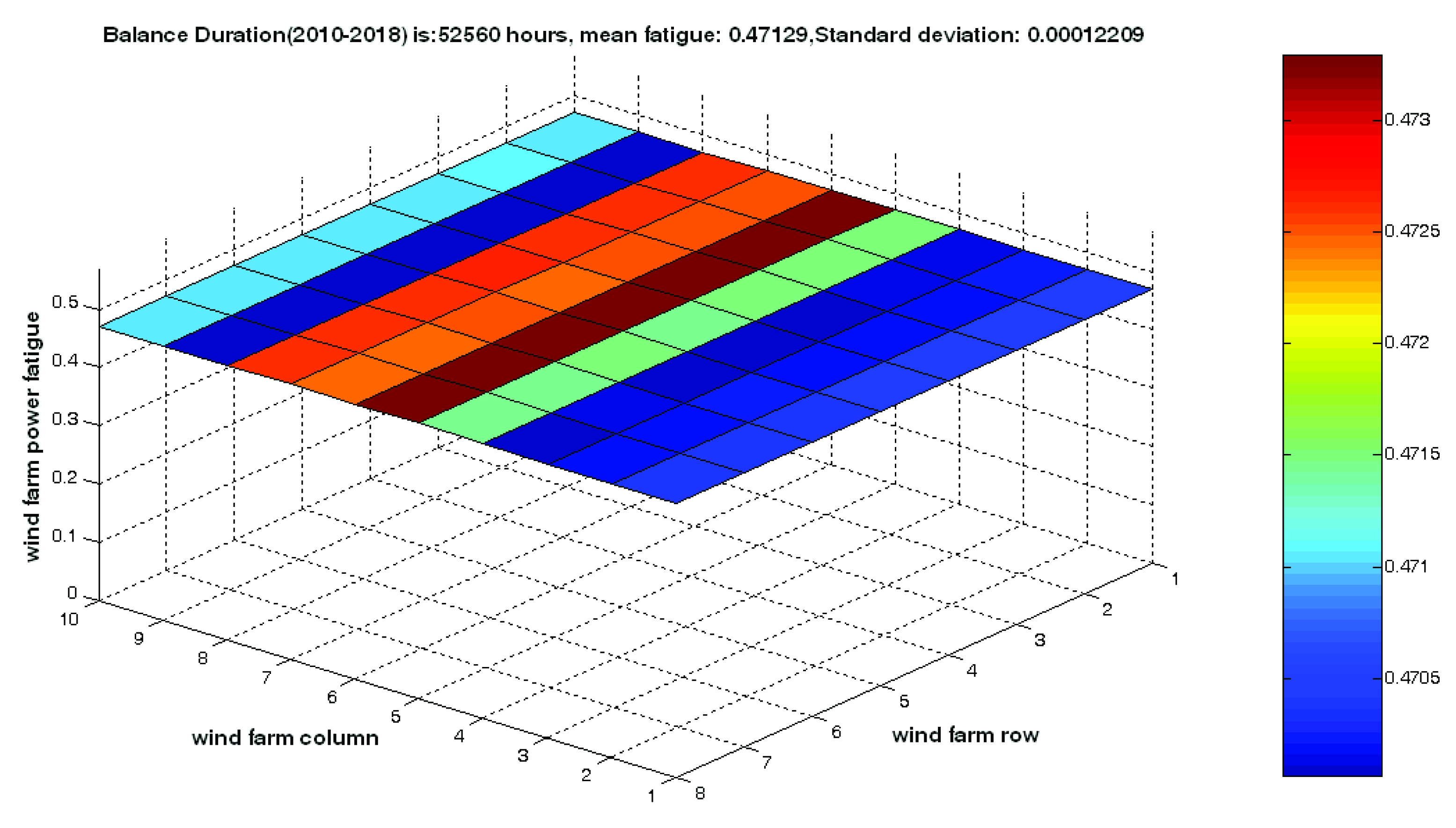
The second case features a simulation with an improved control approach, where the WT fatigue is accumulated using the improved control approach. The optimization result shows that the mean WT fatigue of the whole OWF increases to 0.47129, but the SD of farm fatigue distribution drops to 0.00012209, which means that the WT fatigue distribution is flatter than that using the conventional control in Figure 10, which can save maintenance costs.

7. Discussion

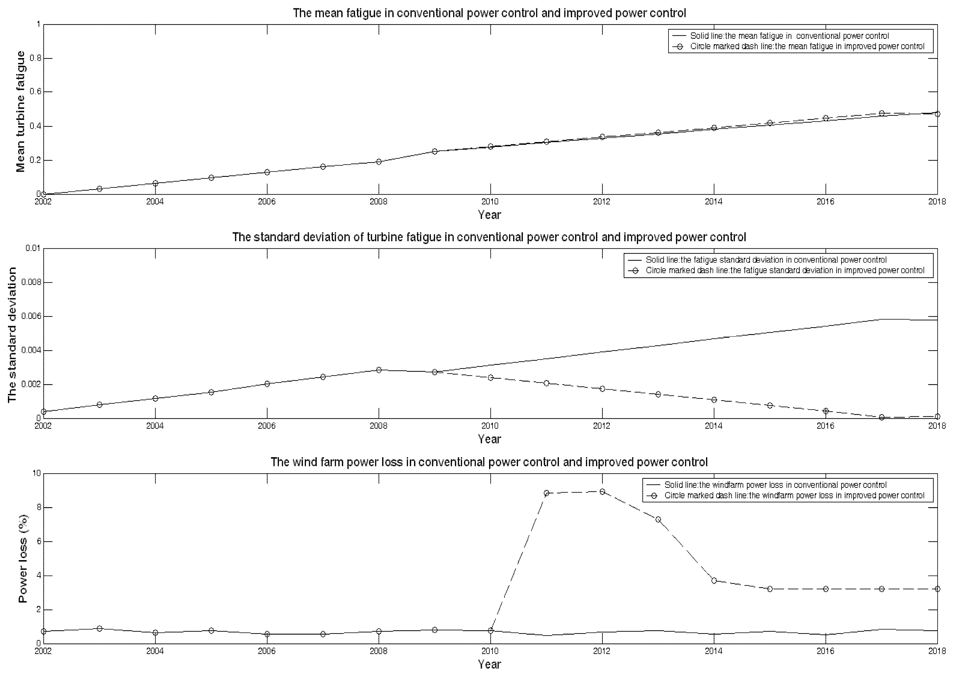
Besides simulations with different control approaches, this study compares the performance of the conventional control WFMC approach and the improved WFMC control approach considering three important parameters: the mean turbine fatigue, the SD of turbine fatigue, and the possible power loss. Figure 11 illustrates different comparisons, where the solid lines denote conventional control and the circle-marked dashed lines denote improved control, during the two simulation stages (2002–2010 and 2010–2018).

As Figure 11 shows, the two mean fatigue curves are nearly the same in both the conventional and improved control approaches. For example, the mean turbine fatigue by 2018 is 0.48001 using the conventional control and 0.47129 under the improved control (i.e., approximately equal). The second parameter, the SD of wind turbine fatigue, is very different for the two control approaches. The SD of wind turbine fatigue keeps increasing up to 0.0057665 by 2018 using the conventional control but decreases gradually to 0.00012209 by 2018 using the improved control. The two curves separate in the year 2010, when the improvement of the WFMC control was made. From this comparison, it is obvious that the flatter this turbine fatigue distribution is, the fewer visits are required by boats or helicopters, leading to a lower maintenance cost.

Wind farm power loss is the factor that has the greatest potential to obstruct such a novel approach during real operations. The power loss of the improved control approach is plotted in the bottom section of Figure 11. During the first duration, the electric power the whole OWF is calculated. In Figure 11, the OWF power loss maintains a mean value of 5.7297% because of the natural wind turbulence from 2002 to 2018. While using the improved power control approach with the same wind data, the power loss in the duration of improved fatigue balance is less than 8.849% in 2010 and reduces to 3.217% by 2018. To some extent, compared with the costs incurred by frequent visits and maintenance, this power generation loss is relatively less, especially in a power-limited state of a WFMC. This assumption should be prove to be true with the future long running duration of the wind farm. In addition, the safety of the maintenance personnel can be further enhanced with a reduced maintenance frequency.

8. Conclusions

The unequal and unbalanced fatigue distribution caused by the wind speed reduction and significant increase in the turbulence level in a far wake is one of causes of the high cost of wind turbines. To reduce this cost, this study presents an improved power control approach to optimize the WT fatigue distribution by balancing the turbulence loads to individual WTs.

This novel power control approach is mainly centered on theoretical research for improving the turbine fatigue definitions, algorithms, WFMC control topologies, and workflows of wind farm main controllers. Sequentially we analyze the conventional power control in a WFMC, as well as the conventional wind turbine fatigue definitions, and then improve the wind turbine fatigue considering together the average wind speed, the turbulence in the turbine wake, and electric power generation.

This study designs a corresponding WFMC control topology and the wind power re-dispatch workflow of a WFMC. The wind direction tolerance values around the main wind angles are calculated depending on the OWF layout geometry, and, finally, this optimization result minimizes the SD of WT fatigue.

The novel power control approach is validated with a simulation of fatigue distribution optimization in one of largest OWFs—the Horns Rev Wind farm-using the wind data stored in the wind characteristics database supported by the Technical University of Denmark. The quantitative fatigue distributions are simulated based on the improved power dispatch approach and illustrated in 3D plots. The simulation results prove that the improved power dispatch approach can reduce the mean turbine fatigue of an OWF, balance the fatigue loads on WTs, further extend the WT lifetime and reduce the potential maintenance costs.