Bi-Level Optimal Strategy of Islanded Multi-Microgrid Systems Based on Optimal Power Flow and Consensus Algorithm

Abstract

Aiming at problems of power allocation and economic scheduling for independent multi-microgrid systems, a bi-level optimization method based on optimal power flow and consensus algorithm is proposed. The novelty of the method is that an independent multi-microgrid system is divided into two layers: in the upper layer, with the predicted output range of the microgrids as the input data, each microgrid is considered as a virtual power supply or virtual load, and taking the minimum network loss as the goal, the energy mutual aid and power allocation among the microgrids are transformed into solving the optimal power flow; in the lower layer, taking the upper layer power distribution scheme as the constraint condition, considering load fluctuation and wind/solar generation uncertainty, the optimal dispatch model of the controllable distributed generator is established based on the distributed theory and the consensus algorithm of equal cost increment, and the "plug and play" of the distributed generator is also realized. An islanded multi-microgrid cluster is taken as an example to verify the economy, security, and reliability of the proposed scheme. The advantages of the scheme have been shown by the simulation example. Simulation results show that the upper-layer method not only realizes the optimal power allocation of microgrids, but also reduces the power loss of the energy mutual aid among the microgrids; through the optimal scheduling of controllable power supply in the microgrid, the lower-level scheme not only improves the economic benefit of the microgrid, but also well suppresses the negative effects of the uncertainties, prediction errors and power fault removal on the multi-microgrid system, which improves the robustness of the system.

1. Introduction

The proliferation of microgrids [1] in distribution networks leads to different types of inter-microgrid connection, such as parallel and series connections, and so on. Compared with a single microgrid, a multi-microgrid system [2] enhances the reliability of the microgrid power supply through energy dispatch and mutual aid of each sub-microgrid and distributed power supply. In addition, mutual energy transfer between each sub-microgrid and distributed generation system can be realized. Although the multi-microgrid system has the advantages of security, reliability, and stability in power distribution and economic dispatch, the complexity of the multi-microgrid system increases due to the connections between the microgrids, which significantly makes power distribution and economical operation of the multi-microgrid system challenging to achieve.

In recent years, researchers have been studying how to achieve optimal power allocation and increase the operational economy and the environmental benefits of power grid systems [3]. In [4], a grid-connected microgrid cluster was studied, and the discrete time first-order consensus algorithm was used to solve the energy management problem of multi-microgrid system. In [5], a hybrid coordinated control strategy combining master-slave with peer-to-peer was adopted in an AC multi-microgrid system. Decentralized power management based on the alternating operation of the multi-segment P/F characteristic curve of the microgrid cluster was realized. In [6], the distributed consensus algorithm was applied to the AC/DC hybrid microgrid, leading to the conclusion that the multi-agent satisfies the plug-and-play principle based on the distributed consistency theory. The feasibility of applying the consensus algorithm to the microgrid was verified in [6]. Reference [7] proposed a novel consensus-based approach to solve the power allocation problem for islanded microgrids. By taking the regulation cost of each agent as the consensus variable and through the exchange of information between adjacent agents, the approach can quickly converge to optimal solutions. In [8], the optimal operation of the active distribution network was realized based on the consensus algorithm, and it was concluded that the optimal economical operation of an active distribution network can be achieved by exchanging local information without a central controller. In [9,10,11], the economic scheduling and coordinated control of a single microgrid were completed based on the consensus algorithm, but did not extend to multi-microgrid systems. In [12], the consensus algorithm was applied to the microgrid cluster system for power allocation, without considering the problem of voltage and frequency stability control of each sub-grid that arises during the process of grid-connection and disconnection. In [13,14], the power distribution of each microgrid in multi-microgrid system was completed based on the game theory, but the network loss problem of energy flow was not considered. References [15,16,17,18] dealt with the coordinated control of voltage, active and reactive power in the lower layers of the microgrid to ensure stable operation of the microgrid based on the consensus algorithm.

In the references mentioned above, the consensus algorithm or game theory were well applied to the microgrid system, solving the problems of energy dispatch, economic operation, coordinated control and so on. However, most of the references did not consider the network loss and the power flow problem in specific nodes of the system during the energy mutual aid. If the optimal power flow (OPF) is solved for all nodes of a multi-microgrid system to achieve the optimal scheduling of the system, then, once the wind and solar generation fluctuate, it is difficult to get the optimal solution or the convergence performance is reduced or even there is no solution. Therefore, this paper presents a bi-level optimization strategy for independent multi-microgrid systems based on optimal power flow and consistency algorithm. The proposed scheme divides the multi-microgrid system into two layers. Taking the predicted output of microgrids as input data and the minimum power flow loss as objective, the upper layer transforms the problem of energy interconnection into the OPF problem to realize power distribution among the microgrids. Considering the load fluctuation and the uncertainty of wind/solar generation in each microgrid, the optimal dispatch model of controllable distributed generator is presented based on the power distribution constraint in the upper layer and the principle of equal-cost incremental rate. The proposed strategy not only reduces the network loss of energy mutual aid among the microgrids, but also suppresses the adverse effects of uncertain factors and prediction errors on the system. Finally, an islanded multi-microgrid system is used as an example to verify the effectiveness, reliability, and superiority of the proposed scheme. Aiming at the forecast output of the microgrids used in the paper, many studies have used the spatio-temporal aware approaches [19], prediction clusters [20] and neural networks [21,22] to study the forecast output of wind/solar, and have achieved good results. However, this paper focuses on the power allocation and economic scheduling of the multi-microgrid system; therefore, the forecast data involved are assumed to have been obtained.

The rest of this paper is organized as follows. Section 2 describes the theoretical basis and mathematical model of the consensus algorithm. Section 3 and Section 4 present the mathematical models of the upper and lower layer of the multi-microgrid system, respectively. Section 5 formulates the management structure of the multi-microgrid system and the solution flow of the bi-level optimal scheduling model. Simulation examples and analysis are presented in Section 6. Finally, conclusions based on the proposed strategy are given in Section 7.

2. Consensus Algorithm

2.1. Graph Theory

The network topology of a multi-microgrid system can be represented by an undirected graph G = (V, E). In this graph, V = {1, 2,..., n} represents each microgrid of the multi-microgrid system, and E represents the communication links between the nodes in the network topology, which indicates the information interaction between each sub-microgrid. An adjacency matrix A = [a_ij] is used to denote the communication relationship between sub-microgrids i and j. If there exists information exchange between sub-microgrids i and j, a_ij= 1; otherwise, a_ij = 0. The Pierre-Simon Laplace matrix L is defined as follows:

$$L=\{\begin{array}{l}{l}_{ii}={\displaystyle \sum _{i\ne j}{a}_{ij}}\\ l_{ij}=-a_{ij}\end{array}$$

(1)

where a_ij represents the corresponding element in the adjacency matrix. The sparse iterative matrix H is defined as

$$h_{ij}=|l_{ij}|/{\displaystyle \sum _{j=1}^n\left|l_{ij}\right|},i=1,2,3,\dots ,n$$

(2)

where h_ij represents the corresponding element in H. If i and j are not adjacent nodes, h_ij = 0.

2.2. Mathematical Model of the Consensus Algorithm

The consensus algorithm of distributed theory can be represented by low-order system or high-order system models. In this paper, a first-order discrete consensus algorithm is used.

For an n-agent system, agent i is chosen as the leading or dominant node, and the remaining nodes are the subordinate nodes. The state of the dominant node i at time t is represented by $x_t^i$, and the dominant node i updates its state information based on $x_t^i$ and the state $x_t^j$ of the adjacent nodes obtained from the communication. The mathematical formula to update the state is shown as

$$x_{t+1}^i={\displaystyle \sum _{j=1}^n{h}_{ij}{x}_t^j}+\delta \cdot \mathsf{\Delta }d$$

(3)

where $\delta$ is the convergence coefficient, and $\mathsf{\Delta }d$ is the deviation of the current state from the steady state.

The state update formula for a non-dominant jth node is shown in (4).

$$x_{t+1}^j={\displaystyle \sum _{i=1}^n{h}_{ij}{x}_t^i,j\ne i}$$

(4)

Similar to (3), if i and j are not adjacent nodes, h_ij = 0.

It can be observed that the state information updates of the dominant node i and the non-dominant node j are related to their previous states and the states of the adjacent nodes. The state of the dominant node needs to be updated constantly based on (3) and (4). However, as it does not require the global information of the whole system, the consensus algorithm helps to avoid excessive communication.

3. Power Mutual Aid Strategy in the Upper Microgrid of Multi-Microgrid System

3.1. Problem Description

A multi-microgrid system is composed of several microgrids. Considering the distance among microgrids, there is power loss in the energy mutual aid between microgrids. In practice, the load demand of a microgrid varies around its rated power. In order to ensure that each microgrid operates normally, a general strategy is based on purchasing electricity directly from the active distribution network when the load is too large. However, in this case, the microgrids with surplus generation capacity are not used, and it is evident that this strategy does not utilize the microgrid resources efficiently. In order to realize mutual energy transfer between sub-microgrids and make full use of their resources, this paper proposes two schemes and compares their performance.

The diagram of a multi-microgrid system consisting of n sub-microgrids is shown in Figure 1.

In such a system, the maximum rated power of a microgrid i is given by ${\overline{P}}_{MGi}$, and its load demand power is represented by $P_{MGi}$.

Scheme One:

According to the forecast value of load and wind/solar generation in each microgrid, power allocation is carried out for each microgrid in the islanded multi-microgrid system by using an equal ratio power-based consensus algorithm. Assuming that ${\overline{P}}_{MGH}$ is the sum of the maximum rated power generated by each microgrid in an islanded multi-microgrid system, i.e.,

$${\overline{P}}_{MGH}={\displaystyle \sum _{i=1}^n{\overline{P}}_{MGi}}$$

(5)

The constant ratio coefficient K of the islanded multi-microgrid system can be defined as follows:

$$K=\frac{{\displaystyle \sum _{i=1}^n{P}_{MGi}}}{{\overline{P}}_{MGH}}$$

(6)

The actual power generation $P_{MGi}^s$ for each microgrid is given by

$$P_{MGi}^s=K\cdot P_{MGi}$$

(7)

It can be seen from (5) and (6) that the output power of each microgrid is determined by its maximum rated power of each microgrid in the power allocation scheme based on the equal ratio power consensus algorithm. Although this scheme balances the overall power in the multi-microgrid system, it is not an optimal scheme as it ignores the problem of line losses between the interconnection among the microgrids.

Scheme Two:

References [23,24] solved the optimal power flow based on the second-order cone programming and solved the problems of optimal scheduling and voltage stability in active distribution networks. In this paper, drawing on this idea and considering the network loss of energy flows among microgrids, an OPF method based on second-order conic programming is proposed to solve the power allocation among the microgrids. Let $\mathsf{\Delta }{P}_{MGi}={\overline{P}}_{MGi}-P_{MGi}$, and the positive $\mathsf{\Delta }{P}_{MGi}$ indicates that the microgrid i has residual power generation capacity. This excess power generation capacity is considered as the maximum rated power generation of a virtual power i, which can be written as $P_{Gi\max }={\overline{P}}_{MGi}-P_{MGi}$. The negative $\mathsf{\Delta }{P}_{MGi}$ shows that the microgrid i needs to purchase energy, and this part of energy is considered as the demand of the virtual load $P_{Li}$, which is written as $P_{Li}=P_{MGi}-{\overline{P}}_{MGi}$. Based on the preceding description, taking the forecast value of wind-solar power generation and load as input, microgrids can be regarded as virtual power or virtual load. The energy mutual aid problem between the microgrids can be transformed into calculating the optimal power flow between n nodes.

Considering that the microgrids are physically separated, the power losses occur during the energy mutual aid process. When calculating the optimal power flow between n nodes, the node with the largest $P_{Gi\max }$ is selected as the balance node. The minimum network loss in the process of the energy mutual aid among microgrids is utilized as the objective function for calculating the OPF and hence obtain the active power $P_{Gi}$ of the virtual power i. Furthermore, the actual power generation $P_{MGi}^s$ corresponding to the microgrid is obtained, thereby completing the optimal coordinated distribution of power and realizing the energy mutual aid between the microgrids.

3.2. Optimal Power Flow Power Allocation Model Based on Second-Order Cone Programming

Interconnecting multiple microgrids can form a multi-microgrid system. Taking the minimum network loss in the process of the energy mutual aid among microgrids as the objective function, the optimal power flow model is established. The objective function is as follows:

$$P_{all,loss}=\min {\displaystyle \sum _{(i,j)\in L}{Z}_{ij}{(I_{ij})}^2}$$

(8)

$$(I_{ij}{)}^2=\frac{{(P_{ij})}^2+{(Q_{ij})}^2}{{(V_i)}^2}$$

(9)

where L represents network branch, $I_{ij}$ represents the current flowing on the branch ij, $Z_{ij}$ represents the impedance of the branch ij, $P_{ij},Q_{ij}$ represent active and reactive power of branch ij, respectively, and $V_i$ is the voltage magnitude of node i.

The active and reactive power balance is expressed in the polar form of the nodal multi-microgrid system power flow equation

$$P_{Gi}-P_{Li}=V_i{\displaystyle \sum _{j=1}^n{V}_j(G_{ij}\cos {\theta }_{ij}+B_{ij}\sin {\theta }_{ij})}$$

(10)

$$Q_{Gi}-Q_{Li}=V_i{\displaystyle \sum _{j=1}^n{V}_j(G_{ij}\sin {\theta }_{ij}-B_{ij}\cos {\theta }_{ij})}$$

(11)

where $P_{Gi}$, $Q_{Gi}$, ($P_{Li}$, $Q_{Li}$) represent the active and reactive powers of generator i (load i), respectively, and $V_i$ and ${\theta }_i$ are the voltage amplitude and phase angle of node i, respectively. The phase angle is given as ${\theta }_{ij}={\theta }_i-{\theta }_j$, and $G_{ij}$ and $B_{ij}$ are the real and imaginary parts of the i-th row and j-th column element of the node admittance matrix, respectively. Let $V_i=e_i+i{f}_i$, then $V_i=\left|V_i\right|(\cos {\theta }_i+i\sin {\theta }_i)$ and $|V{|}^2=e_i^2+f_i^2$. Subsequently, (10) and (11) can be transformed as follows:

$$P_{Gi}-P_{Li}=G_{ii}(e_i^2+f_i^2)+{\displaystyle \sum _{j=1,j\ne i}^n[G_{ij}(e_i{e}_j+f_i{f}_j)-B_{ij}(e_i{f}_j-e_j{f}_i)]}$$

(12)

$$Q_{Gi}-Q_{Li}=-B_{ii}(e_i^2+f_i^2)+{\displaystyle \sum _{j=1,j\ne i}^n[-B_{ij}(e_i{e}_j+f_i{f}_j)-G_{ij}(e_i{f}_j-e_j{f}_i)]}$$

(13)

After the transformation, (12) and (13) become nonlinear and non-convex, which increases the complexity of calculating the OPF. To solve this problem, the second-order cone relaxation technique is introduced to transform (12) and (13) into second-order cones, and the optimal solution is obtained based on the convex programming theory.

Using $c_{ii}=e_i^2+f_i^2$, $c_{ij}=e_i{e}_j+f_i{f}_j$ and $s_{ij}=e_i{f}_j-e_j{f}_i$, (12) and (13) can be converted into

$$P_{Gi}-P_{Li}=G_{ii}{c}_{ii}+{\displaystyle \sum _{j=1,j\ne i}^n(G_{ij}{c}_{ij}-B_{ij}{s}_{ij})}$$

(14)

$$Q_{Gi}-Q_{Li}=-B_{ii}{c}_{ii}+{\displaystyle \sum _{j=1,j\ne i}^n(-B_{ij}{c}_{ij}-G_{ij}{s}_{ij})}$$

(15)

Other constraints are as follows:

$$V_{i\_\min }^2\le c_{ii}\le V_{i\_\max }^2$$

(16)

$$c_{ij}=c_{ji},s_{ij}=-s_{ji}$$

(17)

$$c_{ij}^2+s_{ij}^2=c_{ii}{c}_{jj}$$

(18)

$$P_{Gi\min }\le P_{Gi}\le P_{Gi\max }$$

(19)

$$Q_{Gi\min }\le Q_{Gi}\le Q_{Gi\max }$$

(20)

where $V_{i\_\min }$ and $V_{i\_\max }$ are the maximum and minimum values of the voltage amplitude of the ith node, respectively, $P_{Gi\max }$ and $P_{Gi\min }$ are the maximum and minimum values of the active output of the ith generator, respectively, and $Q_{Gi\max }$ and $Q_{Gi\min }$ are the maximum and minimum values of the reactive output of the ith generator, respectively.

Microgrid i has residual generation capacity and is equivalent to the virtual power; Microgrid j needs to purchase electricity and is equivalent to the virtual load. By solving the optimal power flow, the active power $P_{Gi}$ of the virtual power i can be obtained, that is, the interactive power of the corresponding microgrids. Therefore, the actual power generation of the microgrid i is given by $P_{MGi}^s=P_{MGi}+P_{Gi}$, and the actual power generation of the microgrid j is given by $P_{MGi}^s=P_{MGi}$. By using these calculations, the energy mutual aid between the microgrids is completed, the actual power generation of each microgrid is obtained, and the upper-layer power allocation of the multi-microgrid system is realized.

4. Economic Dispatch of the Lower Level of the Multi-Microgrid System

4.1. Objective Function and Constraints

Microgrids include power generation units, load units and energy storage systems (ESS). Power generation units include controllable units such as micro turbines (MT) and diesel generators (DE), and uncontrolled units such as photovoltaic (PV) and wind turbines (WT). Wind and solar are renewable energies, and their costs are ignored. Using the cost of multi-microgrid system as the optimization objective function, it can be seen that when the operating cost of each sub-microgrid is the lowest, the operating cost of the multi-microgrid system is also the lowest. The objective function is as follows:

$$C=\min {\displaystyle \sum _{i=1}^n{C}_{mgi}}$$

(21)

$$C_{mgi}={\displaystyle \sum _{j=1}^{n}C(P_{MTij})+{\displaystyle \sum _{j=1}^{n}C(P_{DEij})}}+{\displaystyle \sum _{j=1}^{n}C(P_{ESSij})}$$

(22)

where $C_{mgi}$ represents the operating cost of microgrid i; $C(P_{MTij})$ represents the generation cost of MTj in microgrid i; $C(P_{DEij})$ represents the generation cost of DEj in microgrid i; $P_{MTij}$, $P_{DEij}$ and $P_{ESSij}$ represent, respectively, the output power of MTj, DEj and ESSj in microgrid i.

Considering that the generation costs of MT, DE and ESS are all quadratic functions, $P_{DGj}$ is used to represent their output power. Equation (22) can be simplified as follows

$$C_{mgi}={\displaystyle \sum _{j=1}^{n}C(P_{DGij})}$$

(23)

$$C(P_{DGij})=a_{ij}{P}_{DGij}^2+b_{ij}{P}_{DGij}+c_{ij}$$

(24)

where DGij represents MTj, DEj or ESSj in microgrid i; $C(P_{DGij})$ represents the generation cost of MTj, DEj or ESSj in microgrid i; $P_{DGij}$ represents the output power of MTj, DEj or ESSj in microgrid i and $a_{ij},b_{ij},c_{ij}$ represent its cost factors for power generation.

The power balance constraint in sub-microgrid i can be represented as

$${\displaystyle \sum _{j=1}^n{P}_{DGij}+{\displaystyle \sum _{j=1}^n{P}_{WTij}}+{\displaystyle \sum _{j=1}^n{P}_{pvij}}-P_{MGi}-P_{Gi}=0}$$

(25)

The upper and lower limits of the active power of each generator can be written as

$$P_{DGij,\min }\le P_{DGij}\le P_{DGij,\max }$$

(26)

$$P_{WTij,\min }\le P_{WTij}\le P_{WTij,\max }$$

(27)

$$P_{pvij,\min }\le P_{pvij}\le P_{pvij,\max }$$

(28)

where $P_{DGij,\min },P_{DGij,\max }$ represent, respectively, the lower and upper limits of MTj, DEj or ESSj output in microgrid i; $P_{WTij,\min },P_{WTij,\max }$ represent, respectively, the lower and upper limits of WTj, output in microgrid i; $P_{pvij,\min },P_{pvij,\max }$ represent respectively, the lower and upper limits of PVj, output in microgrid i.

4.2. Consensus Algorithm Model Based on Equal Cost Increase Rate

There is wind/solar generation uncertainty, and actual load may fluctuate, i.e.,

$$\mathsf{\Delta }{P}_i={\displaystyle \sum _{j=1}^n{P}_{WTij}}+{\displaystyle \sum _{j=1}^n{P}_{pvij}}-P_{MGi}-P_{Gi}$$

(29)

where $\mathsf{\Delta }{P}_i$ represents the difference value between wind/solar output and load in the microgrid i.

The power balance constraint in microgrid i can be represented as:

$${\displaystyle \sum _{j=1}^n{P}_{DGij}+\mathsf{\Delta }{P}_i=0}$$

(30)

As the cost function is a quadratic function and there are power balance constraints that should be satisfied, the Lagrangian multiplier is introduced. The Lagrange function based on (23) and (30) is given as follows:

$$L(P_{DGi1},P_{DGi2},\dots ,\lambda )=C_{mgi}-\lambda ({\displaystyle \sum _{j=1}^n{P}_{DGij}+\mathsf{\Delta }{P}_i})$$

(31)

where $\lambda$ represents the Lagrange multiplier. The necessary conditions for the existence of Lagrangian extreme value are given by

$$\frac{\partial L}{\partial P_{DGij}}=\frac{\partial C_{mgi}(P_{DGij})}{\partial P_{DGij}}-\lambda =2a_{ij}{P}_{DGij}+b_{ij}-\lambda =0$$

(32)

when $\frac{\partial L}{\partial P_{DGij}}$, the sum of the objective function $C_{mgi}(P_{DGij})$ has a minimum. The value of λ can be obtained from (32) as follows:

$$\lambda =2a_{ij}{P}_{DGij}+b_{ij}$$

(33)

Therefore, it can be concluded that the output of each distributed generator can be obtained using the following expression:

$$P_{DGij}=\frac{\lambda -b_{ij}}{2a_{ij}}$$

(34)

$\lambda$ is selected as a consensus update variable based on equal cost increase rate. The dominant node i is rewritten according to (3) as follows:

$${\lambda }_{r+1}^i={\displaystyle \sum _{j=1}^n{h}_{ij}{\lambda }_r^j+\delta \cdot \mathsf{\Delta }d}$$

(35)

where $\mathsf{\Delta }d={\displaystyle \sum _{j=1}^n{P}_{DGij}+\mathsf{\Delta }{P}_i}$ represents the difference between the current state and the steady state. The variation of $\mathsf{\Delta }d$ is caused by the fluctuation of wind and solar output or deviation of actual load and forecast load.

The non-dominant node j is rewritten according to (4) as follows:

$${\lambda }_{r+1}^j={\displaystyle \sum _{i=1}^n{h}_{ij}{x}_r^i,j\ne i}$$

(36)

The corresponding power generation constraints for each DG are rewritten as

$$P_{DGij}=\{\begin{array}{l}\frac{\lambda -b_{ij}}{2a_{ij}},P_{DGij\min }\le P_{DGij}\le P_{DGij\max }\\ P_{DGij\min },P_{DGij}\le P_{DGij\min }\\ P_{DGij\max },P_{DGij}\ge P_{DGij\min }\end{array}$$

(37)

In the upper layer power allocation of the multi-microgrid system, the energy mutual aid problem between the microgrids is transformed according to (14)–(20) to solve the OPF problem. The actual power generation $P_{MGi}^s$ of each microgrid is obtained from the solution, which is used to constrain power generation for DGs of each microgrid. Therefore, the upper and lower layers are connected, and the power balance is satisfied in each microgrid, which is $P_{MGi}^s={\displaystyle \sum _{j=1}^n{P}_{DGij}}+{\displaystyle \sum _{j=1}^n{P}_{WTij}}+{\displaystyle \sum _{j=1}^n{P}_{pvij}}$. Subsequently, the economic dispatch of DGs in each microgrid is completed by using a consistent algorithm based on an equal cost increase rate. The main steps of the algorithm are as follows:

Step one: The controllable distributed generator i with the highest rated power is selected as the dominant node, and the remaining units represented by j (j ≠ i) are used as the non-dominant nodes in the distributed generator of microgrid.

Step two: The dominant node i updates $\lambda$ according to (35), and the non-dominant node j updates it according to (36) in the rth period. The output power of the corresponding DG is calculated for each update.

Step three: Determine whether $\mathsf{\Delta }d$ is less than the set error ε after completing a cycle. If $\mathsf{\Delta }d$ is less than $\epsilon$, the algorithm ends, and the output corresponds to the active power of each DG. If $\mathsf{\Delta }d$ is not less than $\epsilon$, return to step two to continue the iterative update until $\mathsf{\Delta }d$ is less than $\epsilon$.

It can be seen from the above description that in the islanded multi-microgrid system, the lower layer microgrids use the equal cost increase rate consensus algorithm to obtain the optimal economic dispatching of the distributed generator under the constraint of upper layer power allocation. This process gives the characteristics of “plug and play” and fast communication of the distributed generator in the lower layer.

5. Management Framework of Multi-Microgrid System and Solution Flow of Bi-Level Optimal Scheduling Model

5.1. Management Framework of Upper Layer Microgrids in a Multi-microgrid System

In the multi-microgrid system, each microgrid is an Agent. In the upper layer, the management and control center of multi-microgrid system collects the data of each Agent to know the running state of each microgrid, and then optimizes the power allocation of each microgrid by using the optimization algorithm, so as to give the power allocation instructions to each microgrid. The management and control diagram of the multi-microgrid system is shown in Figure 2:

5.2. Energy Management Framework of the Lower Layer Microgrid in a Multi-Microgrid System

The lower layer microgrid consists of load unit and power generation unit. The microgrid (MG) Agent transmits the information of the load unit and the power generation unit to the management and control center (MCC) of the multi-microgrid system, and also transmits the power allocation instruction issued from the MCC of the multi-microgrid system to the power generation unit. The Agents of MT, DE, ESS, PV and WT exchange information in the power generation unit, and the optimal scheduling is completed by the consensus algorithm. The energy management in the microgrid is shown in Figure 3:

5.3. Solution Flow of Bi-Level Optimal Scheduling Model for Multi-Microgrid System

Taking the predicted output of each microgrid as input data, the interactive power of each microgrid in the upper is calculated by solving the optimal power flow, and the power distribution is completed. With the power distribution of each microgrid as the constraint, the optimal scheduling model of controllable distributed generation in microgrids is solved in the lower layer based on the consensus algorithm of equal cost increment. In the process of bi-level optimization, the lower layer takes priority to suppress load fluctuation or the uncertainty of wind and solar output in each microgrid. If the fluctuation cannot be suppressed (when wind/solar output or load demand changes, the microgrid itself cannot meet the load demand, ${\displaystyle \sum _{j=1}^n{P}_{DGij\max }+\mathsf{\Delta }{P}_i}<0$), the algorithm flow will return to the upper level to resolve. The solution flow chart is shown in Figure 4.

6. Simulation Example

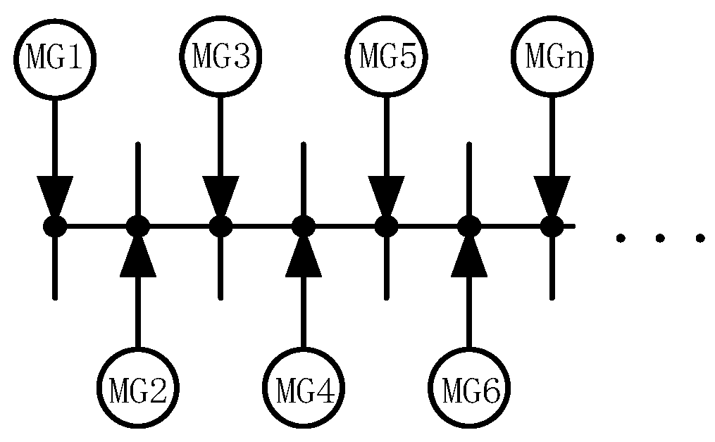
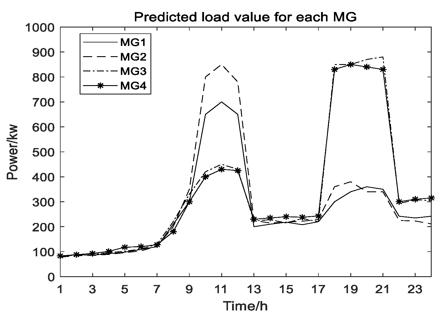
In the simulation example presented in this section, the multi-microgrid system is composed of four microgrids. The maximum rated power generation of MG1, MG2, MG3 and MG4 is 500, 600, 700 and 650 kW, respectively, and the 24-hour forecast load demand of each microgrid is shown in Figure 5.

As can be seen from Figure 5, the forecast load demand peak periods of the multi-microgrid system are between 9:00 and 12:00 and 18:00 and 21:00. Outside the peak periods, there is no need to purchase power from outside as the load demand of each microgrid is less than its maximum power generation. In the period between 10:00 and 12:00, the load demands of microgrid 1 and microgrid 2 exceed their maximum generation power. Therefore, they need to purchase electricity from other microgrids, which include microgrid 3 and microgrid 4, which have excess power generation capacity. In the period between 18:00 and 21:00, the load demand of microgrid 3 and microgrid 4 exceeds their maximum generating power. Therefore, they need to purchase electricity from other microgrids, which include microgrid 1 and microgrid 2 with excess generating capacity. During these two peak periods, each sub-microgrid in the multi-microgrid system requires the energy mutual aid.

6.1. Comparison between OPF Based on Second-Order Cone Programming and Dispatch Based on Equal Ratio Power Consensus Algorithm

Using scheme two described in Section 3.1, the problem of energy exchange between microgrids during the two peak periods is transformed into an OPF problem of the four nodes system. From 9:00 to 12:00, the power to be purchased by microgrid 1 and microgrid 2 is represented as the power demand of virtual loads P_L1 and P_L2, and the excess generation capacity of microgrid 3 and microgrid 4 is represented as the maximum rated generation power of virtual powers P_G3 and P_G4. Similarly, from 18:00 to 21:00, the power to be purchased externally of microgrid 3 and microgrid 4 is considered as the power demand of virtual loads P_L3 and P_L4, and the excess generation capacity of microgrid 1 and microgrid 2 is considered as the maximum rated generation power of virtual powers P_G1 and P_G2.

The results after the nodal processing of prediction data of each microgrid for the two peak periods based on Scheme 2 are shown in

Table 1. The predicted value of virtual power and virtual load for 10:00–12:00.

Time	PL1/kW	PL2/kW	PG3max/kW	PG4max/kW
10:00	150	200	280	250
11:00	200	250	250	220
12:00	150	180	270	225

and

Table 2. The predicted value of virtual power and virtual load for 18:00–21:00.

Time	PL3/kW	PL4/kW	PG1max/kW	PG2max/kW
18:00	150	180	200	240
19:00	150	200	160	220
20:00	170	190	140	260
21:00	180	180	150	260

.

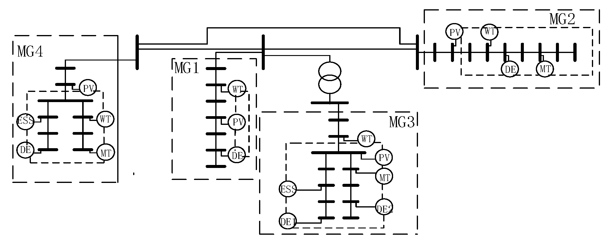
Through data processing, the microgrids during the time periods of 10:00–12:00 and 18:00–21:00 are either converted into virtual load or virtual power. The multi-microgrid system corresponding to the two peak periods is shown in Figure 6.

Referring to the standard data of the IEEE 4 node system, the line parameters of multi-microgrid system are shown in

Table 3. Line parameters.

	Node i	Node j	R	X
Line parameter	1	2	0.1	0.4
	1	4	0.12	0.5
	2	4	0.08	0.4

and

Table 4. Transformer parameters.

	Node i	Node j	R	X	k	$\underset{\_}{k}$	$\overline{k}$
Transformer parameter	1	3	0	0.3	0.909091	0.9	1.15

.

All the parameters in the Table 3 and Table 4 are per unit value. Nodes 1–4 represent the PCC nodes connected by microgrids 1–4. R and X represent the resistance and reactance between node i and node j, respectively; k represents the per unit ratio of the transformer, and $\overline{k},\underset{\_}{k}$ represent its upper and lower limits.

In the multi-microgrid system, the node with the maximum P_Gimax is selected as the balance node, and the data in Table 1 and Table 2 are used to calculate OPF based on second-order cone programming. The final results are shown in

Table 5. Virtual power active output and network loss for 10:00–12:00.

	10:00	11:00	12:00
PG3	211 kW	250 kW	202.6 kW
PG4	144.8 kW	207.5 kW	132.6 kW
network loss	5.8 kW	7.5 kW	5.3 kW

and

Table 6. Virtual power active output and network loss for 18:00–21:00.

	18:00	19:00	20:00	21:00
PG1	200 kW	160 kW	140 kW	150 kW
PG2	132.2 kW	192.9 kW	223.2 kW	212.9 kW
network loss	2.2 kW	2.9 kW	3.2kW	2.9 kW

.

Using the data in Table 5 and Table 6, the value of the objective function that gives the minimum value of network loss can be calculated. By solving the OPF, the active power of virtual power corresponding to the output power of the microgrid and the network loss are obtained.

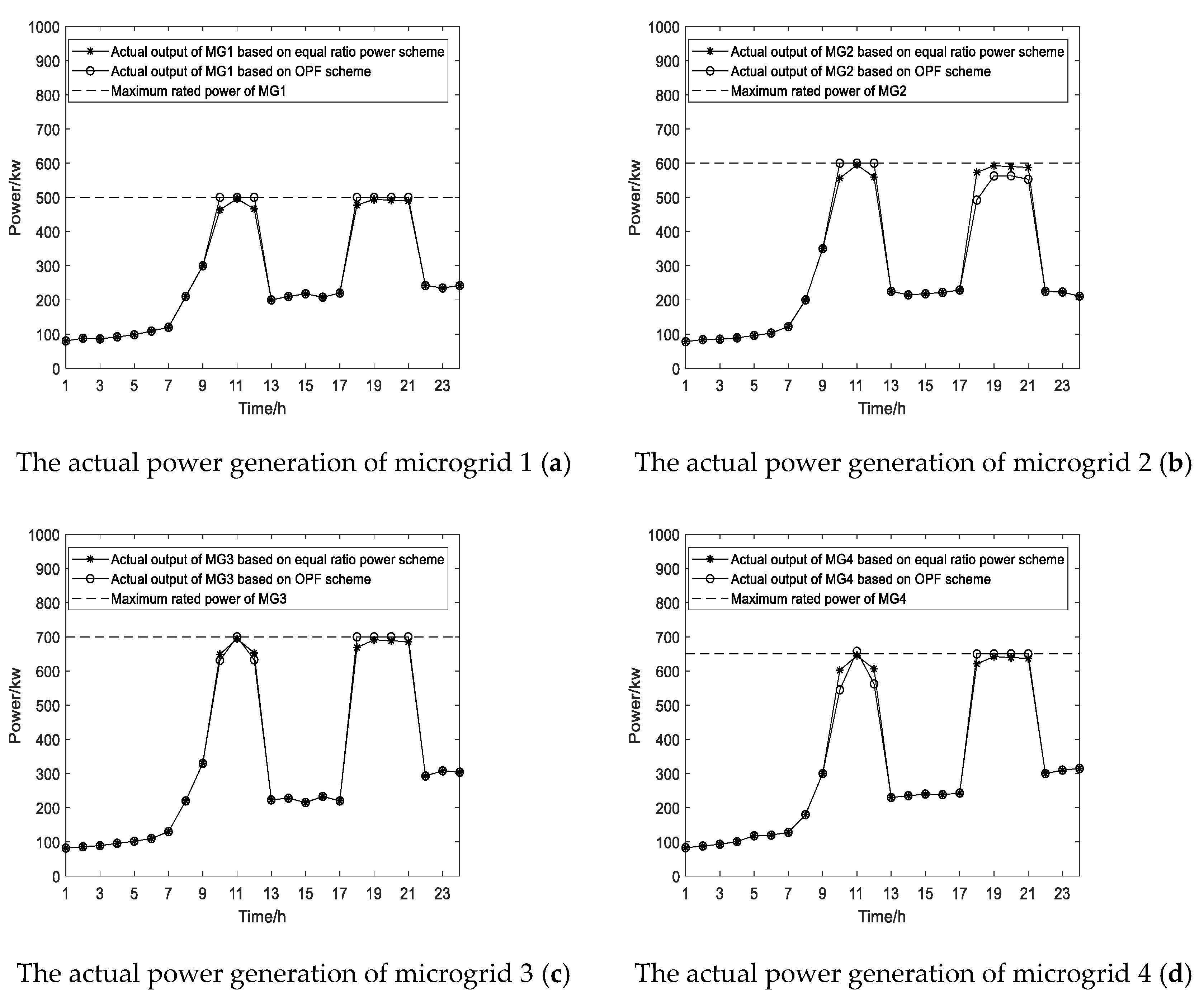
Using scheme one described in Section 3.1, after allocating the power of each microgrid in the upper based on the equal ratio power consensus algorithm, the actual generation power of each microgrid for 24 hours is obtained. The comparison results with the OPF scheme based on second-order cone programming in scheme two are shown in Figure 7.

The corresponding network losses of the two schemes between 10:00 and 12:00 and 18:00 and 21:00 are shown in

Table 7. Network loss of the two schemes for 10:00–12:00.

	10:00	11:00	12:00
Network loss ofthe upper layeroptimal power flow scheme	5.8 kW	7.5 kW	5.3 kW
Network loss ofthe upper layerequal ratiopowerscheme	7.2 kW	7.7 kW	6.4 kW

and

Table 8. Network loss of the two schemes for 18:00–21:00.

	18:00	19:00	20:00	21:00
Network loss ofthe upper layer optimal power flow scheme	2.2 kW	2.9 kW	3.2 kW	2.9 kW
Network loss ofthe upper layer equal ratiopower scheme	3.1 kW	3.2 kW	3.6 kW	3.5 kW

.

It can be observed from Figure 7a,b that during the 10:00–12:00 period, based on the OPF scheme, microgrids 1 and 2 as power purchasers achieved the maximum power generation and resource utilization. By using the equal ratio scheme, the power distribution of each microgrid is realized under the condition of the power balancing of each microgrid in the multi-microgrid system. However, as power purchasers, the power output of microgrids 1 and 2 is not maximized, which means that the power needed to be purchased from other microgrids will increase, resulting in a more significant network loss. It can be concluded from the data shown in Table 7 and Table 8 that the network loss obtained using the equal ratio power scheme is higher than that using the OPF scheme.

As shown in Figure 7c,d, during 18:00–21:00, under the condition of power balancing of each microgrid in the multi-microgrid system, the OPF scheme results in optimal energy mutual aid economic dispatch of each microgrid while minimizing the energy mutual aid network loss of each microgrid. As power purchasers, microgrids 3 and 4 achieve maximum power and resource utilization. According to the data shown in Table 7 and Table 8, the network loss obtained using the OPF scheme is lower than that based on the equal ratio power scheme.

Based on the above discussion, it can be concluded that in the islanded multi-microgrid system, the OPF scheme based on second-order cone programming can reduce the loss of each microgrid occurring during the process of energy exchange. In addition, it can also achieve the optimal power coordination distribution and power balance of each microgrid.

6.2. Economic Dispatch of Distributed Generators in the Lower Layer Microgrid

The actual generating power of each microgrid can be obtained when the energy exchange of each microgrid in the upper layer is complete. At this time, the economic cost in each microgrid is taken as the target, and it is optimized using the consensus algorithm of equal cost increase rate.

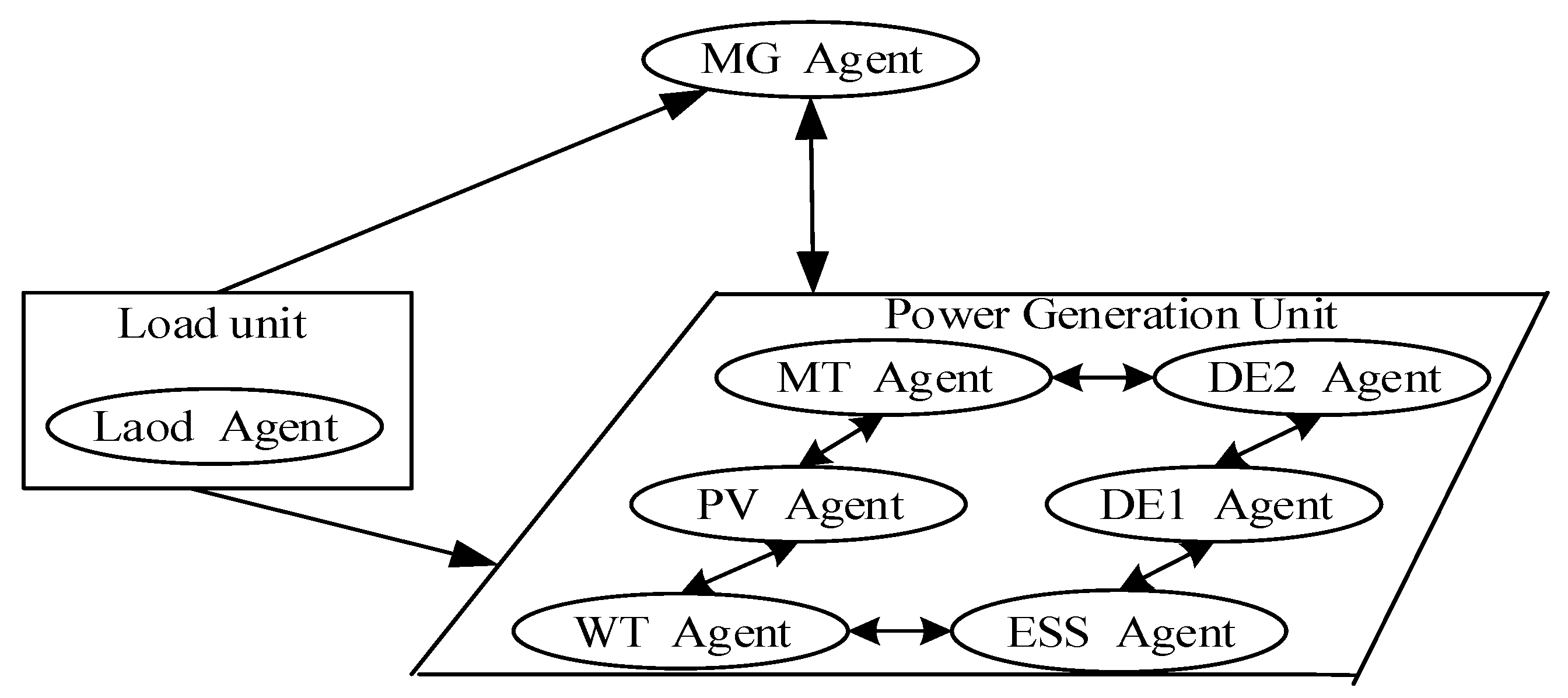
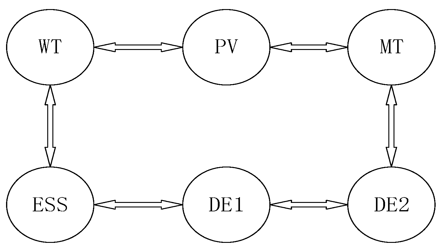
Taking the microgrid 3 as an example, the communication topology of its distributed generators is shown in Figure 8.

The generation cost coefficient and upper and lower generation limits of each distributed generator are shown in

Table 9. Characteristic parameters of DG.

DG	a/($/kW2h)	b/($/kWh)	c/($/h)	PGijmin/kW	PGijmax/kW
ESS	0.095	0	0	−100	100
DE1	0.0081	5.72	63	0	100
MT	0.0064	5.54	47	0	100
DE2	0.0081	5.72	63	0	100

. In the following, three different operating scenarios are considered.

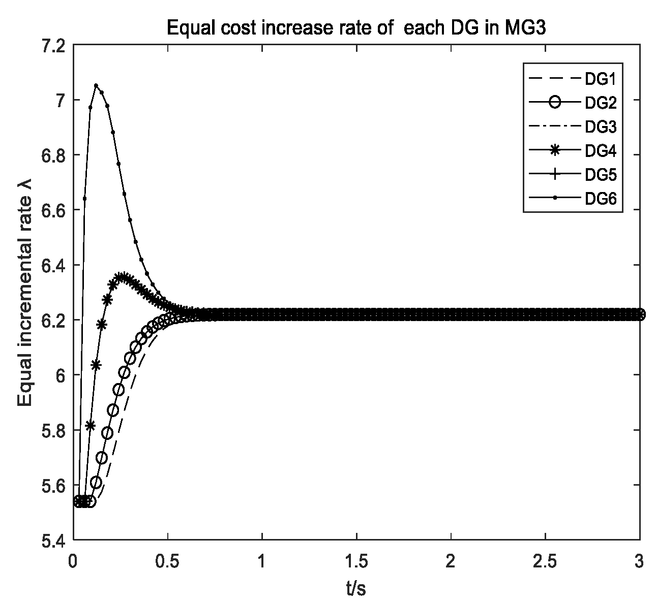
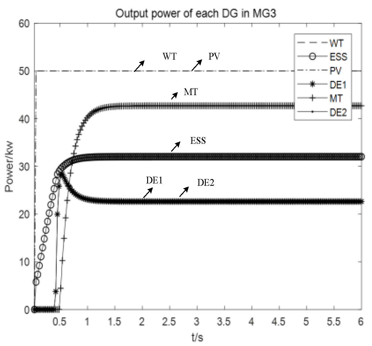
(1) Microgrid 3 and Distributed Generators Operating Normally

The power demand of microgrid 3 is 220 kW at 8:00. When all the distributed generators in the network are working regularly, simulation results obtained using the consensus algorithm based on equal cost increase rate are shown in Figure 9 and Figure 10.

It can be observed from Figure 9 that the equal cost increase rate of each DG converges to the same value at 0.8 s. In Figure 10, the output powers of the DGs after convergence at 0.8 s are equal to 53.0414, 30.7982, 30.7982, 30.7982, 53.0414, and 21.5226 kW, while the total power is 220 kW, which satisfies the power balancing constraint. The economic state of microgrid 3 is the optimum at this time.

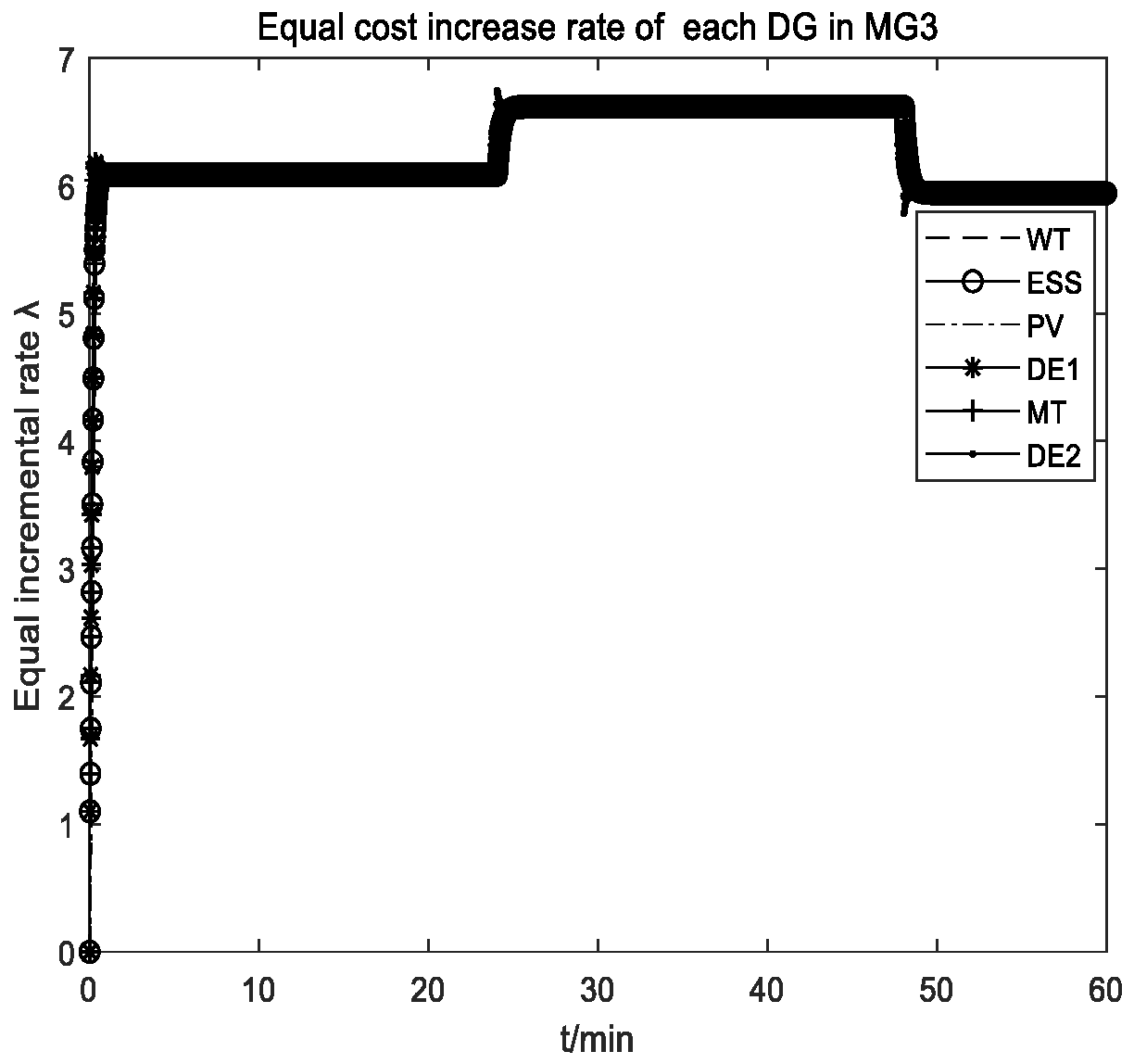
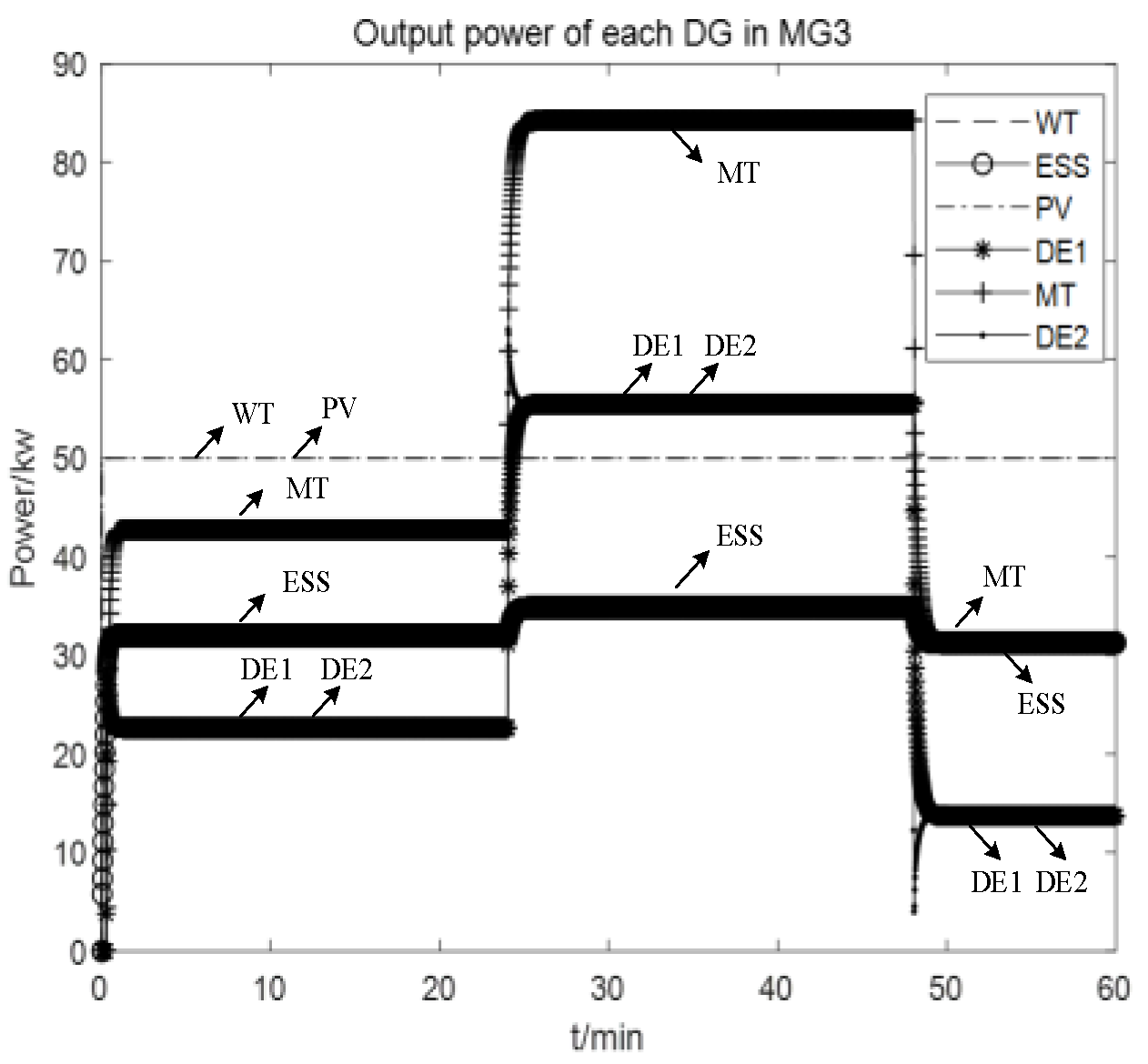
(2) Fluctuation of load demand in MG3

From 8:00 to 9:00, the load demand of MG3 fluctuates from 220 to 330 kW, then from 330 to 190 kW. Based on the consensus algorithm of equal cost increase rate, the output power of each distributed generator becomes stable again. The simulation results are shown in Figure 11 and Figure 12.

It can be observed from the simulation results that when the load demand power of microgrid 3 increases from 220 to 330 kW at 8:25, the distributed generators in the microgrid will adjust according to the updated information of the load demand and the equal cost increase rate converges again in 1.5 s. The output powers of distributed generators after achieving balance are 74.8493, 48.0291, 48.0291, 48.0291, 74.8493, and 36.2143 kW, while the total power is 330kW, which meets the power balancing constraint. When the load demand power of microgrid 3 drops from 330 to 190 kW at 8:48, the distributed generators in the microgrid will adjust according to the updated information of the load demand, and the equal cost increase rate converges again. The output powers of distributed generators after achieving balance are 50, 31.2715, 50, 13.6776, 31.3733, and 13.6776 kW, meeting the power balancing constraint. Therefore, load fluctuation in MG3 is suppressed, and the adverse influence of its on multi-microgrid system is reduced.

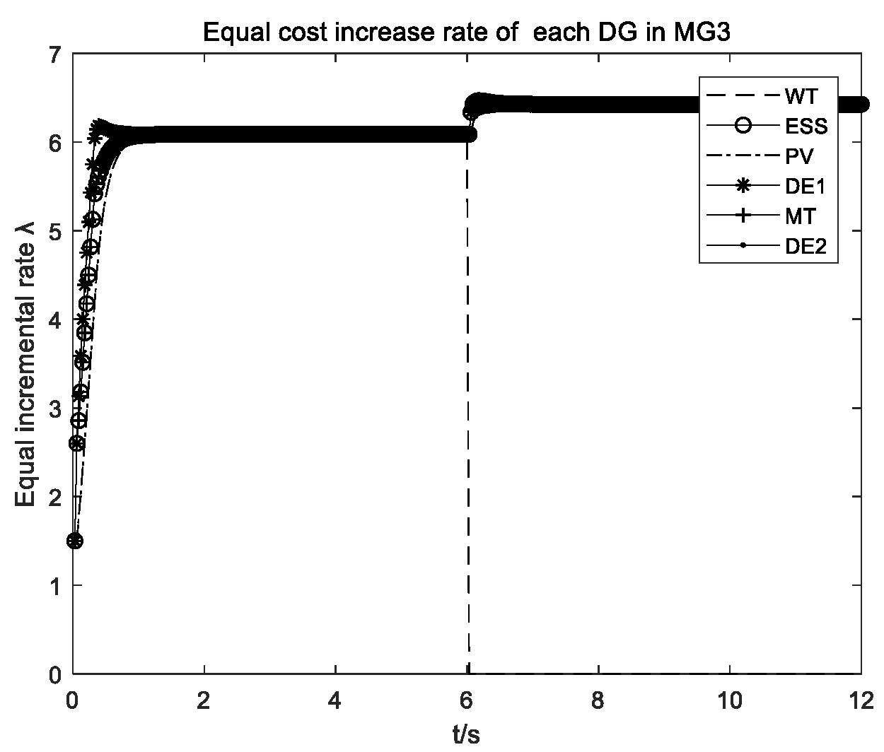
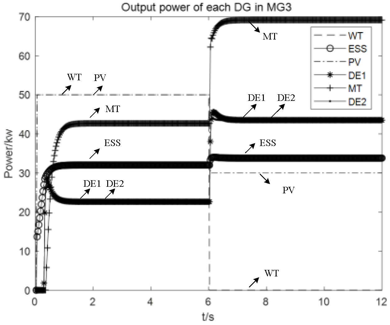
(3) The Output Power of PV Reduced, Exit of WT from Network Topology Due to Failure

From 8:00 to 9:00, the power demand of microgrid 3 is 220 kW. At some point, PV power drops from 50 to 30 kW due to insufficient light intensity and a fault occurs in WT. The power demand of the microgrid 3 is 220 kW at 8:00. When the running state of microgrid 3 is stable, DG1 exits the network topology due to malfunction, and the corresponding simulation results are shown in Figure 13 and Figure 14.

Based on the simulation results, it can be concluded that when the wind turbine exits the network topology, the corresponding equal cost increase rate and output power become zero. The remaining five distributed generators exchange information, and the equal incremental rate converges within 0.6s. The output power of each DG after achieving stability is 41.1613, 41.1613, 41.1613, 66.1574 and 30.3587 kW, while the total power is 220 kW, which meets the power balance constraint. Therefore, the uncertainty of wind and solar output in microgrid 3 is also suppressed, and the adverse influence of its on multi-microgrid system is greatly reduced.

6.3. Efficiency Analysis of Simulation Program

All examples in this article were run on a Lenovo computer with an I7 processor and 8G operating memory. The upper code for optimal power flow model was written with Matlab2017, and then the power flow model was transformed into second-order cone by Yalmip toolbox, and solved by Gurobi; the lower layer code of the consensus algorithm model based on the equal cost incremental rate was also written with Matlab; at last, all the optimized results were illustrated by Visio 2013. The running time and memory occupied by the upper and lower models are shown in

Table 10. Upper model program run time and required RAM.

Time	Program Running Time	RAM
10:00	0.711675 s	5060 MB
11:00	0.740310 s	5069 MB
12:00	0.691015 s	5100 MB
18:00	0.745581 s	5254 MB
19:00	0.894457 s	5203 MB
20:00	0.841057 s	5199 MB
21:00	0.682764 s	5272 MB

Note: In other periods, each microgrid can meet the load demand itself. Energy mutual aid among microgrids is not needed, so it is not necessary to calculate the optimal power flow.

and

Table 11. Lower model program run time and required RAM.

Simulation of Section 6.2	Program Running Time	RAM
Simulation 1	0.328165 s	5275 MB
Simulation 2	0.368797 s	5280 MB
Simulation 3	0.336205 s	5245 MB

:

7. Conclusions

Aiming at problems of power allocation and economic scheduling for independent multi-microgrid systems, a bi-level optimization method based on optimal power flow and consensus algorithm is proposed. In this method, independent multi-microgrid system is divided into two layers: in the upper layer, taking the predicted output range of microgrids as input data, each microgrid is considered as a virtual power supply or virtual load, and considering the minimum power flow loss, a solution to the problem of power allocation among microgrids is presented. The solution transforms the energy mutual aid between microgrids to achieve optimal power flow, which leads to optimal power mutual aid distribution among the microgrids. In the lower layer, considering load fluctuation and wind/solar generation randomness in the microgrids, the power allocation scheme of the upper layer is utilized as the constraint condition, and the micro-increase rate of equal cost is taken as the consensus variable for each microgrid in the lower layer. The consensus algorithm is used to establish the optimal scheduling model of the controllable distributed generations in each microgrid, which resulted in the microgrid operating stably in the optimal state. Finally, an islanded multi-microgrid cluster with four MGs is taken as an example to verify the proposed strategy. Simulation examples are provided to verify that the bi-level optimization method reduces the power loss of the energy mutual aid between microgrids in the upper layer and completes the optimal power distribution among the microgrids; the internal algorithm of the microgrids in the lower layer realizes the optimal scheduling of the controllable distributed generators. When there is a prediction error due to the load fluctuations and the uncertainty of wind/solar output, the controllable distributed generators in the microgrid quickly adjust its power output through information exchange and can still quickly converge again and reach power balance. The negative impact of the microgrid internal uncertainty on the multi-microgrid system is well suppressed, and the "plug and play" of distributed power in the microgrid is also achieved. Therefore, the proposed strategy can greatly improve the economy, reliability, and robustness of the islanded multi-microgrid system.

There are still some shortcomings in this paper: due to the limitation of resource conditions, the simulation examples made by the paper only include four microgrids, and they have not been extended to a larger multi-microgrid system. In addition, the scheme proposed in this paper has only been verified using simulation examples and has not yet been validated in practical multi-microgrid systems.

References

1. Parhizi, S.; Lotfi, H.; Khodaei, A.; Bahramirad, S. State of the Art in Research on Microgrids: A Review. IEEE Access 2015, 3, 890–925. [Google Scholar] [CrossRef]
2. Meng, L.; Shafiee, Q.; Trecate, G.F.; Karimi, H.; Fulwani, D.; Lu, X.; Guerrero, J.M. Review on Control of DC Microgrids and Multiple Microgrid Clusters. IEEE J. Emerg. Sel. Top. Power Electron. 2017, 5, 928–948. [Google Scholar]
3. Zhang, Y.; Fang, J.; Wang, S.; Yao, H. Energy-water nexus in electricity trade network: A case study of interprovincial electricity trade in China. Appl. Energy 2020, 257, 1–11. [Google Scholar] [CrossRef]
4. Huang, B.; Li, Y.; Zhang, H.; Sun, Q. Distributed optimal co-multi-microgrids energy management for energy internet. IEEE J. Autom. Sin. 2016, 4, 357–364. [Google Scholar]
5. Xiong, X.; Wu, M.; Ji, Y.; Sun, L. Power Management and Coordinated Control Strategy Research of Multi-microgrids. Proc. CSEE 2018, 38, 1419–1427. [Google Scholar]
6. Gao, Y.; Ai, Q.; Wang, J. Consensus Cooperative Control of AC/DC Hybrid Microgrids Based on Multi-agent System. High Volt. Eng. 2018, 44, 2372–2377. [Google Scholar]
7. Tang, Z.; Hill, D.J.; Liu, T. A Novel Consensus-Based Economic Dispatch for Microgrids. IEEE Trans. Smart Grid 2018, 9, 3920–3922. [Google Scholar] [CrossRef]
8. Pu, T.; Wei, L.; Chen, N.; Wang, X. Distributed Optimal Dispatching of Active Distribution Network Based on Consensus Algorithm. Proc. CSEE 2017, 37, 1579–1590. [Google Scholar]
9. Wang, R.; Li, Q.; Zhang, B.; Wang, L. Distributed Consensus Based Algorithm for Economic Dispatch in a Microgrid. IEEE Trans. Smart Grid 2019, 10, 3630–3640. [Google Scholar] [CrossRef]
10. Kim, H.-M.; Hussain, A.; Kim, H.-M. Diffusion Strategy-Based Distributed Operation of Microgrids Using Multiagent System. Energies 2017, 10, 903. [Google Scholar]
11. Lyu, Z.; Wei, Q.; Zhang, Y.; Zhao, J.; Manla, E. Adaptive Virtual Impedance Droop Control Based on Consensus Control of Reactive Current. Energies 2018, 11, 1801. [Google Scholar] [CrossRef] [Green Version]
12. He, H.; Fang, L.; Han, B.; Li, G. A Consensus Protocol Based Control Method for Coordinated Multi-Microgrid Control. Power Syst. Technol. 2017, 41, 1269–1276. [Google Scholar]
13. Li, Y.; Zhao, T.; Wang, P.; Gooi, H.B.; Wu, L.; Liu, Y.; Ye, J. Optimal Operation of Multi-Microgrids via Cooperative Energy and Reserve Scheduling. IEEE Trans. Ind. Inform. 2018, 14, 3459–3468. [Google Scholar] [CrossRef]
14. Xiao, L.; Mandayam, N.B.; Poor, H. Prospect Theoretic Analysis of Energy Exchange among Microgrids. IEEE Trans. Smart Grid 2015, 6, 63–72. [Google Scholar] [CrossRef]
15. Liu, Z.; Wu, Z.; Dou, X.; Hu, M. A Distributed Droop Control Scheme for Islanded DC Microgrid Considering Operation Costs. Proc. CSEE 2016, 36, 900–910. [Google Scholar]
16. Lu, X.N.; Guerrero, J.M.; Sun, K.; Vasquez, J.C. An improved droop control method for DC microgrids based on low bandwidth communication with DC bus voltage restoration and enhanced current sharing accuracy. IEEE Trans. Power Electr. 2014, 29, 1800–1812. [Google Scholar] [CrossRef] [Green Version]
17. Zhang, H.; Kim, S.; Sun, Q.; Zhou, J. Distributed Adaptive Virtual Impedance Control for Accurate Reactive Power Sharing Based on Consensus Control in Microgrids. IEEE Trans. Smart Grid 2016, 8, 1–13. [Google Scholar] [CrossRef]
18. Schiffer, J.; Seel, T.; Raisch, J.; Sezi, T. Voltage Stability and Reactive Power Sharing in Inverter-Based Microgrids With Consensus-Based Distributed Voltage Control. IEEE Trans. Control Syst. Technol. 2015, 24, 96–109. [Google Scholar] [CrossRef] [Green Version]
19. Bessa, R.; Trindade, A.; Miranda, V. Spatial-Temporal Solar Power Forecasting for Smart Grids. IEEE Trans. Ind. Inform. 2015, 11, 232–241. [Google Scholar] [CrossRef]
20. Corizzo, R.; Pio, G.; Ceci, M.; Malerba, D. DENCAST: Distributed density-based clustering for multi-target regression. J. Big Data 2019, 6, 1–27. [Google Scholar] [CrossRef]
21. Ceci, M.; Corizzo, R.; Malerba, D.; Rashkovska, A. Spatial autocorrelation and entropy for renewable energy forecasting. Data Min. Knowl. Discov. 2019, 33, 698–729. [Google Scholar] [CrossRef]
22. Abdel-Nasser, M.; Mahmoud, K. Accurate photovoltaic power forecasting models using deep LSTM-RNN. Neural Comput. Appl. 2019, 31, 2727–2740. [Google Scholar] [CrossRef]
23. Yibing, L.; Wenchuan, W.U.; Boming, Z.; Li, Z. A Mixed Integer Second-order Cone Programming Based Active and Reactive Power Coordinated Multi-period Optimization for Active Distribution Network. Proc. CSEE 2014, 34, 2575–2583. [Google Scholar]
24. Li, Y.; Xiao, J.; Chen, C.; Tan, Y.; Cao, Y. Service Restoration Model with Mixed-Integer Second-Order Cone Programming for Distribution Network with Distributed Generations. IEEE Trans. Smart Grid 2019, 10, 4138–4150. [Google Scholar] [CrossRef]
Figure 1. Multi-microgrid system topology.
Energies 13 01537 g001
Figure 2. Management framework of upper microgrids.
Energies 13 01537 g002
Figure 3. Energy management framework in the microgrid.
Energies 13 01537 g003
Figure 4. Solving flow chart of bi-level optimal scheduling model.
Energies 13 01537 g004
Figure 5. The forecast load demand of each microgrid over 24 hours.
Energies 13 01537 g005
Figure 6. Topology of multi-microgrid system.
Energies 13 01537 g006
Figure 7. The actual power generation of each microgrid over 24 hours.
Energies 13 01537 g007
Figure 8. DG communication topology.
Energies 13 01537 g008
Figure 9. Equal cost increase rate of each DG.
Energies 13 01537 g009
Figure 10. Output power of each DG.
Energies 13 01537 g010
Figure 11. Equal cost increase rate of each DG.
Energies 13 01537 g011
Figure 12. Output power of each DG.
Energies 13 01537 g012
Figure 13. Equal cost increase rate of each DG.
Energies 13 01537 g013
Figure 14. Output power of each DG.
Energies 13 01537 g014