A Framework for Flexible and Cost-Efficient Retrofit Measures of Heat Exchanger Networks

Abstract

Retrofitting of industrial heat recovery systems can contribute significantly to meeting energy efficiency targets for industrial plants. One issue to consider when screening retrofit design proposals is that industrial heat recovery systems must be able to handle variations, e.g., in inlet temperatures or heat capacity flow rates, in such a way that operational targets are reached. Consequently, there is a need for systematic retrofitting methodologies that are applicable to multi-period heat exchanger networks (HENs). In this study, a framework was developed to achieve flexible and cost-efficient retrofit measures of (industrial) HENs. The main idea is to split the retrofitting processes into several sub-steps. This splitting allows well-proven (single period) retrofit methodologies to be used to generate different design proposals, which are collected in a superstructure. By means of structural feasibility assessment, structurally infeasible design proposals can be discarded from further analysis, yielding a reduced superstructure. Additionally, critical point analysis is applied to identify those operating points within the uncertainty span that determine necessary overdesign of heat exchangers. In the final step, the most cost-efficient design proposal within the reduced superstructure is identified. The proposed framework was applied to a HEN retrofit case study to illustrate the proposed framework.

1. Introduction

After the Paris Agreement 2015, decarbonization of industry and energy-intensive industrial processes has been proposed as one of the key measures to limit the increase of the global average temperature well below 2 °C. Within decarbonization of industry, waste heat recovery is dedicated to play a major role.

Systematic approaches to design and synthesize heat recovery systems, especially heat exchanger networks (HENs), have been subject to research since the early 1980s with the introduction of the graphical Pinch analysis method [1]. In addition to the graphical Pinch analysis method, mathematical programming has been well established as a complementary approach to HEN synthesis. Both sequential approaches [2] and simultaneous approaches [3], where targeting and network synthesis are performed separately and simultaneously, respectively, have been developed and reported in the literature. In addition, hybrid methods, which combine graphical methods and mathematical programming [4], have been suggested. Among others, Axelsson et al. [5], Bengtsson et al. [6], as well as Escobar and Trierweiler [7] have applied graphical and mathematical methods to case studies, including industrial applications, and reported results and comparisons.

The above-mentioned methods do not account for the variation and uncertainty in operating data that often occur in industrial applications. One example is the variation of input conditions for HENs, i.e., temperatures and flowrates, but also uncertainty in design characteristics, such as heat transfer coefficients of heat exchangers (HEXs). The consequences of neglecting these variations and uncertainties as well as using average or nominal values for design purposes can be increased utility demand (see, e.g., [8]). Additionally, more severe operability issues may occur, e.g., the controllability of target values may not be guaranteed. In order to face these challenges, different strategies have been proposed and a good overview is provided by Kang and Liu [9] in their recent review paper on the synthesis of flexible HENs. Some literature is mentioned here. Kotjabasakis and Linnhoff [10] developed an approach to mitigate the unwanted response of a HEN to variations based on sensitivity tables and systematic utilization of downstream paths. Hafizan et al. [11] utilized the plus-minus principle, introduced by Linnhoff and Vredeveld [12], to visualize the impact of process modifications on the minimum utility target, to derive heuristics for HEN design synthesis based on graphical methods if the respective HEN is subject to disturbances in inlet temperatures.

In addition to graphical approaches (e.g., Pinch-based), mathematical programming has great potential when dealing with variations and uncertainty in operating data. Floudas and Grossmann [13] introduced a multi-period approach to the HEN synthesis problem, which was automated [14] and developed further in the late 1980s [15]. More recently, the multi-period approach has been developed further by a number of authors. In this context, Aaltola [16] extended the SYNHEAT model of Yee and Grossmann [3] to multiple periods. Additionally, Verheyen and Zhang [17] as well as Short et al. [18] improved the model of Aaltola [16] by considering more specific HEX design data. The multi-period HEN synthesis strategy was further applied by Tveit et al. [19] to industrial applications.

Compared to the synthesis of HENs for greenfield problems, the rearrangement of an existing HEN (retrofitting problem) is a different problem. In contrast to greenfield design situations, a retrofitting problem is often characterized by additional constraints and limitations. Extensive work exists on retrofitting methodologies based on graphical insights (e.g., Lai et al. [20], Kamel et al. [21], Bonhivers et al. [22]), mathematical programming (e.g., Ciric and Floudas [23], Asante and Zhu [24], Athier et al. [25]), and those methodologies that can be characterized as hybrid methodologies combining graphical analysis and mathematical programming (e.g., Smith et al. [26], Jiang et al. [27], Akpomiemie and Smith [28]). A comprehensive overview on different retrofitting methodologies can be found in [29].

The above-mentioned retrofit methodologies for HENs do not account for variations and uncertainties in operating data, e.g., in inlet temperatures or heat capacity flowrates. Usually, steady-state or average values are considered, i.e., the reported methodologies are suited for retrofitting single-period HENs, only. However, the capability to account for variations and uncertainties is essential in certain industry applications. Persson and Berntsson [8] showed that considering annual average values to calculate the steam savings potential of a retrofit heat integration project in a pulp mill can lead to an overestimation of 15% compared to the steam savings potential calculated with monthly average values. Persson and Berntsson further concluded in [30] that the steam savings potential decreases even further if it is calculated with average values of shorter time periods (e.g., daily or 10-min periods). In contrast to the results reported by Persson and Berntsson as well as the excessive amount of methodologies available for retrofitting single-period HENs, little attention has been paid to HEN retrofit methodologies that account for variations and uncertainties in operating data. It is worth mentioning that this imbalance between only a few methodologies for multi-period HEN retrofit in comparison with the reported methodologies for single-period HEN retrofit was observed by authors previously publishing in the field (see, e.g., [31]). In fact, to our knowledge, only two systematic retrofitting methodologies for multi-period HENs are reported in the literature. These two retrofitting methodologies are described in the following paragraph.

Papalexandri et al. [32] developed a multi-period Mixed Integer (Non-)Linear Program (MI(N)LP) model, which is based on multi-period hyperstructures, including the considered retrofit alternatives. Furthermore, Papalexandri et al. [32] proposed an iterative scheme between the developed multi-period MI(N)LP and a flexibility analysis subproblem to identify the retrofit alternative, which is operable over a priori defined variations and yields the minimum total annualized cost. Another retrofitting methodology was reported by Kang and Liu [31], who introduced a two-step method to achieve retrofit design proposals that can operate cost efficiently at multiple periods. In a first step, the multi-period HEN synthesis model as it is used in greenfield design problems is employed. In the second step, existing exchangers are relocated in order to meet the required area demands identified in step one.

Although the above-mentioned retrofit approaches account for variations and uncertainty in operating data, there are several reasons why these approaches are not easily applied to large and complex industrial applications. Commonly, complexities, such as splitting or recirculation of streams, are present in industrial heat recovery systems, which cause nonlinearities in the mathematical formulation of these systems. Therefore, the resulting multi-period MINLP, including retrofit design proposals incorporated as hyper structures as proposed in [32], becomes complex, which inevitably leads to difficultness in finding feasible solutions. Additionally, the flexibility analysis subproblem for large and complex industrial applications is difficult to solve even with state-of-the-art global MINLP solvers. Moreover, depending on the problem complexity itself, the solution produced by common multi-period HEN synthesis formulations and the current network layout may differ essentially. Consequently, relocating existing exchangers to meet identified area demands as proposed in [31] can easily result in inefficient trial and error procedures.

The above reported methodologies are based on mathematical programming, which coincides with the benefits of mathematical programming when dealing with variations in operating data. However, in comparison to these methodologies, graphical insights-based methods have great potential to be applied to large and complex applications due to their beneficial user interaction. Recently, different strategies have been reported in the literature to utilize approaches based on graphical insights in the design process of multi-period HEN retrofitting case studies. A common strategy to deal with variations in operating conditions from a Pinch analysis perspective is to develop different retrofit proposals for a number of selected sets of operating conditions (e.g., annual, seasonal, and monthly average values) [8]. The different design proposals are then evaluated and may be combined to achieve an, over all considered operating points, operable and energy-efficient retrofit proposal. Another strategy is to develop different retrofit proposals by employing graphical insights-based retrofitting methods (e.g., Bridge analyses [22] or advanced composite curves [33]) for a specific nominal point and analyze the network’s response to variations to obtain insights and identify the best performing retrofit design proposal [34]. Additionally, Langner et al. [35] proposed to decouple the design and analysis steps in retrofitting processes. By means of this decoupling, well-proven (single period) retrofit design methodologies can be utilized to generate different design proposals, which thereafter are evaluated and adjusted in a trial and error manner with respect to flexibility and energy efficiency [35]. In conclusion, approaching a retrofit problem subject to variations in operating data from a Pinch analysis perspective relies to a large extent on trial and error procedures as different design proposals must be evaluated and manually combined. Good results can be obtained, but the design process itself is often very inefficient due to the trial and error character of the respective strategies.

As pointed out, systematic methodologies for retrofitting industrial HENs subject to variation in operating data are needed, but the available methodologies fulfill this demand only partly. Therefore, we propose a new framework in this paper to achieve flexible and cost-efficient retrofit measures by combining the beneficial designer interaction of graphical approaches (e.g., Pinch based) at an early stage in the design process with the efficiency of mathematical programming. By means of this combination, inefficient trial and error procedures can be avoided. The proposed framework is based on single-period (e.g., Pinch based) retrofit methodologies, (structural) flexibility analysis, critical point analysis, and multi-period optimization. The proposed framework is outlined in Section 3 of this paper. In the following section, the theoretical background of (structural) flexibility analysis and critical point analysis is provided.

2. Theoretical Background

2.1. (Structural) Flexibility Analysis

Flexibility analysis of HENs has been subject to research since the early 1980s. In 1982, Marselle et al. [36] first introduced the concept of resilient HENs with respect to a certain disturbance range in the inlet conditions. In 1985, Saboo et al. [37] introduced a resilience index to quantify the resilience of HENs. In the same year, Swaney and Grossmann [38] extended the concept of the resilience index to a flexibility index, which is applicable not only to HENs but also to chemical processes in general. Both the resilience and the flexibility index indicate the maximum disturbance range in which inlet conditions may vary while at the same time achieve feasible operation. This maximum disturbance range can be interpreted as a hyperrectangle in the space of the varying inlet conditions. In this context, both indices are defined as the ratio between the largest scaled hyperrectangle within the feasible region and the hyperrectangle defined by an expected disturbance range. Therefore, feasibility is achieved if the respective index is larger or equal to 1. For two varying inlet conditions, this can be visualized as in Figure 1. The largest scaled rectangle within the feasible region can mathematically be expressed by the following set of equations ($\mathsf{\delta }$ corresponds to flexibility/resilience index):

$${\mathrm{T}}_{1,\mathrm{N}}-\mathsf{\delta }\ast \mathsf{\Delta }{\mathrm{T}}_1^{-}\le {\mathrm{T}}_1\le {\mathrm{T}}_{1,\mathrm{N}}+\mathsf{\delta }\ast \mathsf{\Delta }{\mathrm{T}}_1^{+},$$

(1)

$${\mathrm{T}}_{2,\mathrm{N}}-\mathsf{\delta }\ast \mathsf{\Delta }{\mathrm{T}}_2^{-}\le {\mathrm{T}}_2\le {\mathrm{T}}_{2,\mathrm{N}}+\mathsf{\delta }\ast \mathsf{\Delta }{\mathrm{T}}_2^{+}.$$

(2)

In Figure 1, the largest scaled rectangle within the feasible region is smaller than the rectangle according to the expected variations. Thus, feasibility with respect to the expected variations is not achieved (flexibility or resilience index is smaller than 1). In both index formulations, the physical performance of the HEN or the chemical process is described by the following set of constraints:

$${\mathrm{h}}_{\mathrm{i}}\left(\mathrm{d},\mathrm{x},\mathrm{z},\mathsf{\Theta }\right)=0;\mathrm{i}\in \mathrm{I},$$

(3)

$${\mathrm{g}}_{\mathrm{j}}\left(\mathrm{d},\mathrm{x},\mathrm{z},\mathsf{\Theta }\right)\le 0;\mathrm{j}\in \mathrm{J},$$

(4)

where d is the vector of design variables, x corresponds to the state variables, z is used for the control variables, and the varying inlet conditions or uncertain parameters are depicted by Θ (see [37,38]). In HENs, typical design variables are the area values of HEXs while typical uncertain parameters are the inlet temperatures or heat capacity flow rates of process and/or utility streams. State and control variables correspond to the internal network temperatures and duties of HEX. Furthermore, the operational equality constraints of HENs are heat and mass balances while operational inequality constraints ensure a minimum temperature difference as well as that heat transfer is only possible from hot to cold streams. Additionally, design constraints of HEXs (in form of heat transport equations) may also be considered as operational inequality constraints.

Feasibility is achieved when all constraints $\mathrm{i}\in \mathrm{I}$ and $\mathrm{j}\in \mathrm{J}$ are satisfied at the point of operation. With both formulations, it is possible to describe the resilience or flexibility for convex problems in which the solution lies at a vertex point of the largest scaled (hyper-)rectangle within the feasible region (see Figure 1). In 1987, Grossmann and Floudas [39] developed an active set approach to guarantee a global solution of the flexibility index problem also for some non-convex problems. More recently, Li et al. [40] suggested a framework to calculate the flexibility index by means of an alternating direction matrix embedded in a simulated annealing algorithm. Furthermore, Zhao and Chen [41] proposed to explicitly calculate the shape of the uncertainty space via cylindrical algebraic decomposition and quantifier elimination.

In the context of flexibility analysis of HENs, the term structural flexibility is used to define the set of constraints that are included in the flexibility analysis. Often, it is distinguished between structural constraints (e.g., heat and mass balances) and design constraints (e.g., heat transport equations of HEX). Marselle et al. [36] distinguished, for example, between a resilient network structure and a resilient network itself. Marselle et al. [36] further suggest that a network structure is resilient if it remains feasible for the specified disturbance range independent of the HEX areas (i.e., HEX areas are not specified). A resilient network structure is, thus, the premise for a resilient network, which remains feasible for the specified disturbance range for specified HEX areas [36]. This definition of structural resilience was later used by Li et al. [42] to describe the structural flexibility of HENs. In accordance with the literature, our work distinguishes between the structural feasibility of a design and the (general) feasibility of a design. Both can be assessed by solving the flexibility index problem. In the case of structural feasibility assessment, design constraints are discarded, and only structural constraints are considered, i.e., the heat transferred by HEXs is not limited by design characteristics. In the case of (general) feasibility assessment, design constraints are included, i.e., the heat transferred by HEXs is limited by design characteristics (i.e., the installed surface area and the overall heat transfer coefficient of exchangers).

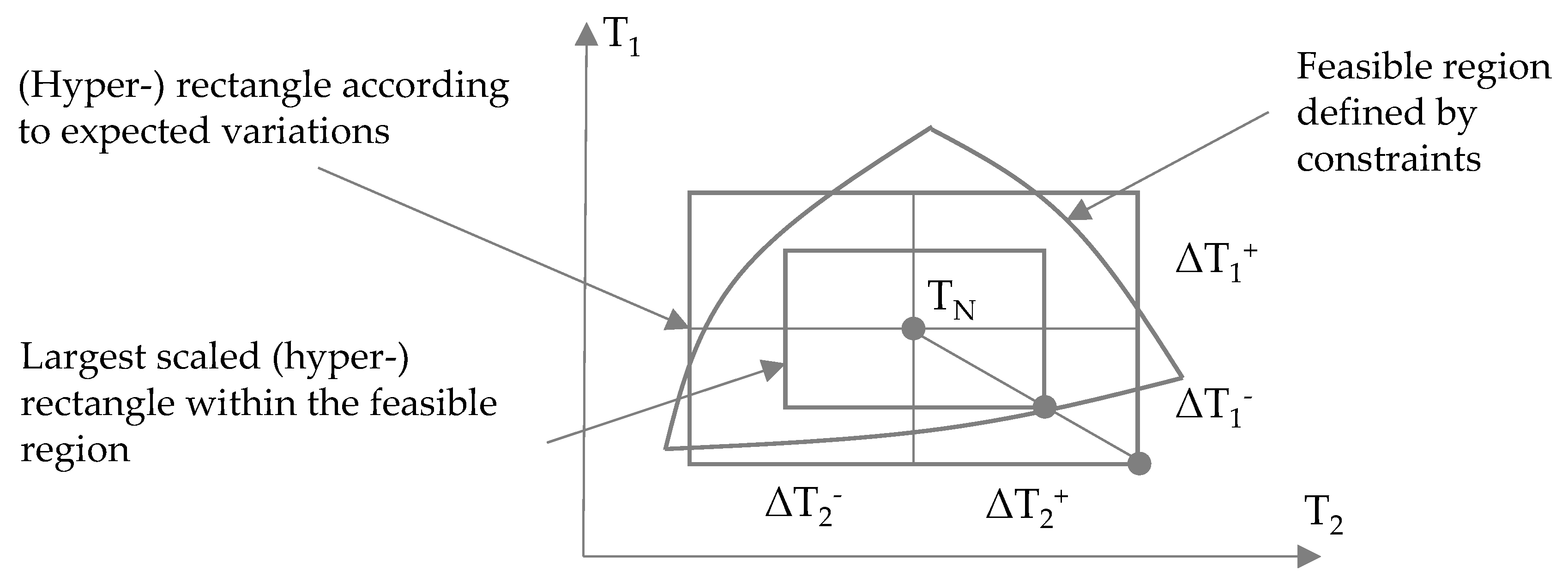
2.2. Multi-Period Design Problem and Critical Point Analysis

In a multi-period design problem, independently of the chosen approach, sufficiently many sets of operating points need to be considered to guarantee the flexibility and cost efficiency of the achieved solution. However, with an increasing number of sets of operating points, the complexity of the problem increases. Especially for large-scale industrial applications, the computational capacity can be a limiting factor. To overcome these difficulties, different works in the literature deal with the reduction of the sets of operating points, e.g., by sensitivity analyses [43] or by the identification of critical operating points [44] of a given design proposal. The main idea of these approaches is to identify those variations (within a given uncertainty span) of the uncertain parameters, which require the largest equipment size and are, thus, critical for the design and operation of the HEN. This implies that the HEN itself must be structurally feasible and the feasibility may only be limited by design characteristics, i.e., HEX surface area and heat transfer coefficients (see Section 2.1). The identified critical operating points can be utilized to find the necessary overdesign of HEXs in a fixed HEN structure. By including the identified critical points in the design problem, feasibility for the entire uncertainty span can be achieved. Additionally, representative operating points/scenarios may be identified, e.g., by the screening of historical data, and included in the design problem to achieve a cost-efficient solution (cost optimal for the set of critical points and representative operating points/scenarios). In conclusion, the design problem subject to critical and representative operating points/scenarios can be expressed as the following multi-period MI(N)LP optimization problem:

$$\begin{array}{l}\underset{\mathrm{x},\mathrm{z},\mathrm{d}}{\min }\mathrm{TAC}={\displaystyle {\displaystyle \sum }_{\mathrm{s}\in \mathrm{S}}}\left[{\mathrm{w}}_{\mathrm{s}}{\ast \mathrm{c}}_{\mathrm{operating},\mathrm{s}}\right]+{\mathrm{c}}_{\mathrm{investment}}\ast \mathrm{CRF}\\ \mathrm{s}.\mathrm{t}.\\ \begin{array}{l}{\mathrm{h}}_{\mathrm{i}}\left(\mathrm{x},\mathrm{z},\mathrm{d},{\mathsf{\theta }}_{\mathrm{op}}\right)=0;\mathrm{i}\in \mathrm{I}\\ {\mathrm{g}}_{\mathrm{j}}\left(\mathrm{x},\mathrm{z},\mathrm{d},{\mathsf{\theta }}_{\mathrm{op}}\right)\le 0;\mathrm{j}\in \mathrm{J}\\ {\mathrm{g}}_{\mathrm{d}}\left(\mathrm{x},\mathrm{z},{\mathsf{\theta }}_{\mathrm{op}}\right)-\mathrm{d}\le 0;\mathrm{d}\in \mathrm{DV}\\ \mathrm{d}\ge 0\\ \mathrm{x},\mathrm{z},\mathrm{d},{\mathsf{\theta }}_{\mathrm{op}}\in \mathrm{R},{ \mathsf{\theta }}_{\mathrm{L}}\le {\mathsf{\theta }}_{\mathrm{op}}\le {\mathsf{\theta }}_{\mathrm{U}}\end{array}\}\mathrm{op}\in \left(\mathrm{S}\cup \mathrm{CP}\right).\end{array}$$

(5)

In (5), $\mathrm{TAC}$ represents the total annualized cost of the HEN design, which is described by the annual operating cost ${\mathrm{c}}_{\mathrm{operating}}$ in €/year (utility cost) of a number of defined representative operating points/scenarios $\mathrm{s}\in \mathrm{S}$, which are weighted with their normalized duration factor ${\mathrm{w}}_{\mathrm{s}}$ (time period represented by operating point divided by entire time period), and the investment cost ${\mathrm{c}}_{\mathrm{investment}}$ in € (e.g., HEX investment cost), which are annualized with a given capital recovery factor $\mathrm{CRF}$. The set of equality constraints is depicted by ${\mathrm{h}}_{\mathrm{i}}$ with $\mathrm{i}\in \mathrm{I}$ (heat and mass balances) and the set of inequality constraints is represented by ${\mathrm{g}}_{\mathrm{j}}$ with $\mathrm{j}\in \mathrm{J}$ (temperature and other operational restrictions). The set of design constraints ${\mathrm{g}}_{\mathrm{d}}$ depends on the set of the non-negative design variables $\mathrm{d}$ with $\mathrm{d}\in \mathrm{DV}$. In ${\mathrm{h}}_{\mathrm{i}}$, ${\mathrm{g}}_{\mathrm{j}}$, and ${\mathrm{g}}_{\mathrm{d}}$, $\mathrm{x}$ is the vector of the state variables, $\mathrm{z}$ corresponds to the control variables, and the varying inlet conditions or uncertain parameters are depicted by $\mathsf{\theta }$. Consequently, in order to find the optimal value for $\mathrm{TAC}$ (for the respective operating points), the degrees of freedom of the optimization problem are the non-negative design variables $\mathrm{d}$ with $\mathrm{d}\in \mathrm{DV}$ and the control variables (of the HEN) $\mathrm{z}$. The set of constraints must be satisfied at all representative operating points/scenarios $\mathrm{s}\in \mathrm{S}$ and at all identified critical operating points $\mathrm{c}\in \mathrm{CP}$, i.e., for certain, previously identified, fixed combinations of values for the uncertain parameters. In (5), the set of constraints must be satisfied at each operating point present in the union of the two sets $\mathrm{S}$ and $\mathrm{CP}$: $\mathrm{op}\in \left(\mathrm{S}\cup \mathrm{CP}\right)$. This way, a flexible and cost-efficient design is achieved.

To identify those variations (within a given uncertainty span) that require the largest equipment size, sensitivity analyses can be used if monotonic correlations between uncertain parameters and design variables exist. One example is the correlation between the uncertain heat transfer coefficient and the surface area of a HEX—the maximum area of the HEX is obtained at the smallest value of the heat transfer coefficient within the uncertainty span [45]. However, it can be assumed that not many parameters follow these clear correlations and critical operating points can be determined following the procedure introduced by Pintarič and Kravanja in [44], which is based on the following idea:

“The main idea is to identify points with the largest values of design variables at optimum objective function. This may be achieved by maximizing design variables one by one, while allowing uncertain parameters to obtain any value between the specified bounds, and simultaneously minimizing cost function.”

[44] (p. 1607)

This implies a max-min problem for each design variable $\mathrm{d}\in \mathrm{DV}$, i.e., maximizing the design variable of interest ${\mathrm{d}}_{\mathrm{i}}$ while minimizing the cost function $\mathrm{C}\left(\mathrm{x},\mathrm{z},\mathrm{d},\mathsf{\theta }\right)$, which is stated in problem (6). Compared to the cost function in (5) ($\mathrm{TAC}$), in the cost function of (6) ($\mathrm{C}\left(\mathrm{x},\mathrm{z},\mathrm{d},\mathsf{\theta }\right)$), the operating cost of the representative operating points is not included:

$$\begin{array}{l}\underset{\mathsf{\theta }}{\max {\mathrm{d}}_{\mathrm{i}}}=\underset{\mathrm{x},\mathrm{z},\mathrm{d}}{\min }\mathrm{C}\left(\mathrm{x},\mathrm{z},\mathrm{d},\mathsf{\theta }\right)={\mathrm{c}}_{\mathrm{operating}}+{\mathrm{c}}_{\mathrm{investment}}\ast \mathrm{CRF}\\ \mathrm{s}.\mathrm{t}.\\ {\mathrm{h}}_{\mathrm{i}}\left(\mathrm{x},\mathrm{z},\mathrm{d},\mathsf{\theta }\right)=0;\mathrm{i}\in \mathrm{I}\\ {\mathrm{g}}_{\mathrm{j}}\left(\mathrm{x},\mathrm{z},\mathrm{d},\mathsf{\theta }\right)\le 0;\mathrm{j}\in \mathrm{J}\\ \mathrm{d}={\mathrm{g}}_{\mathrm{d}}\left(\mathrm{x},\mathrm{z},\mathsf{\theta }\right);\mathrm{d}\in \mathrm{DV}\\ \mathrm{x},\mathrm{z},\mathrm{d},\mathsf{\theta }\in \mathrm{R}, \mathrm{d}\ge 0,{ \mathsf{\theta }}_{\mathrm{L}}\le \mathsf{\theta }\le {\mathsf{\theta }}_{\mathrm{U}}.\end{array}$$

(6)

To solve the max-min problem, Pintarič and Kravanja [44] developed different formulations:

• The Karush–Kuhn–Tucker (KKT-) formulation;
• The two-level formulation; and
• The approximate one-level formulation.

By means of these formulations, possible candidates for critical points are identified. In a second step, a set covering algorithm is applied to the identified candidates to merge them into a final set of critical points. Both the two-level and the approximate one-level formulation approximate the solution of the KKT-formulation. Moreover, the approximate one-level formulation is dependent on a heuristically chosen Big-M parameter and solutions can be very sensitive to this parameter. Additionally, if the system is convex, all critical points are vertices of the uncertain space. These critical vertices can be identified by solving problem (5), excluding the representative operating points, sequentially at all vertices. Those vertices at which the maximum values for each design variable are obtained are critical [44].

3. Methodology

In order to achieve retrofit design proposals that can operate cost efficiently at multiple operating points, a framework was developed. The framework is shown in Figure 2 and will be outlined in the following subsections. The proposed framework utilizes single-period and well-proven retrofit design methodologies but also “experience-based” retrofit design proposals can be considered. Design proposals that are structurally infeasible are discarded after a structural feasibility assessment. To avoid suboptimal solutions due to unnecessary overdesign of equipment, the proposed framework is based on the identification of critical points. Cost efficiency for the entire operating period is ensured, by considering representative operating points besides the identified critical points when solving the eventual design problem. A final feasibility check is performed to ensure that all critical points have been identified (i.e., the set of critical points is complete); otherwise, the new critical point, which is identified during this check, is added to the set of critical point(s) and the design problem is solved again.

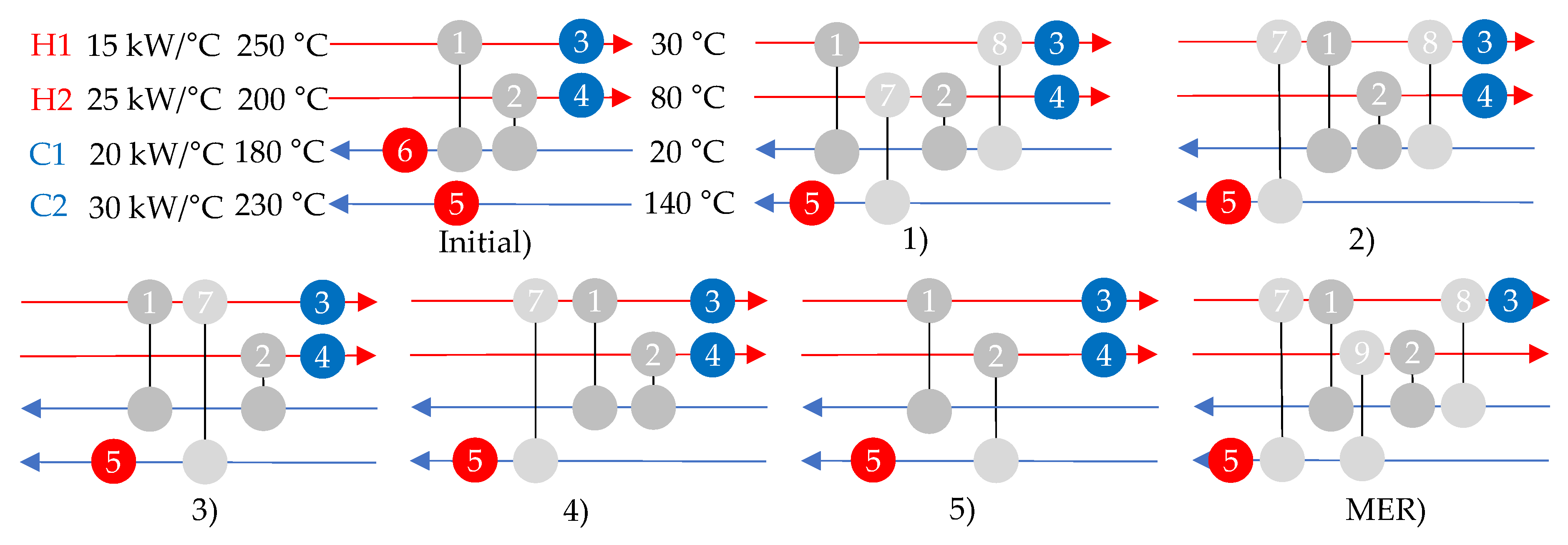
3.1. HEN Retrofit Design Proposals for Single Operating Point—Generation of Superstructure

In a first step, retrofit design measures are derived using single-period and well-proven retrofit design methodologies. Additionally, “experience-based” design proposals may be considered, which can be based on, e.g., already known operability issues. By means of this, the designer is actively involved in the design process, which can be beneficial in industrial applications. The derived design changes are collected in a superstructure, which eventually represents all design proposals that are considered.

3.2. Structural Feasibility Assessment—Reduction of Superstructure

In the next step, the structural feasibility of the identified proposals is analyzed. As outlined in Section 2.1, this can be done by calculating the flexibility index discarding all design constraints and considering only structural constraints. The flexibility index can be calculated using the active set approach developed by Floudas and Grossman [39]. However, the active set approach may result in impractical large problem formulations as industrial applications are often complex. Alternative formulations exist, such as the calculation of the flexibility index via the direction matrix [40] or via cylindrical algebraic decomposition and quantifier elimination [41]. However, the first alternative relies on the simulated annealing algorithm, which means that the global solution may not be found in a reasonable period of time. Moreover, applying cylindrical decomposition to industrial applications (which typically involve more than four HEXs and uncertain parameters) requires excessive computational capacity, which may not be available. An alternative is Monte Carlo network simulations with random variations within the uncertainty span while degrees of freedom are utilized to control operational targets and minimize utility cost in a similar way as it was proposed by Kachacha et al. in [46]. With an increasing number of uncertain parameters and complexity of the problem, computational capacity is the limiting factor for this approach. Although all listed methodologies for (structural) feasibility assessment have known drawbacks, it is assumed that structural feasibility assessment of HENs (also in more complex industrial applications) is possible. To reduce the probability of faulty results, the authors suggest applying several of the proposed methods and compare the achieved results. If design proposals can be identified that are structurally infeasible for at least some operating points within the uncertainty span (i.e., flexibility index smaller than 1), these design proposals are excluded from the superstructure, yielding a reduced superstructure.

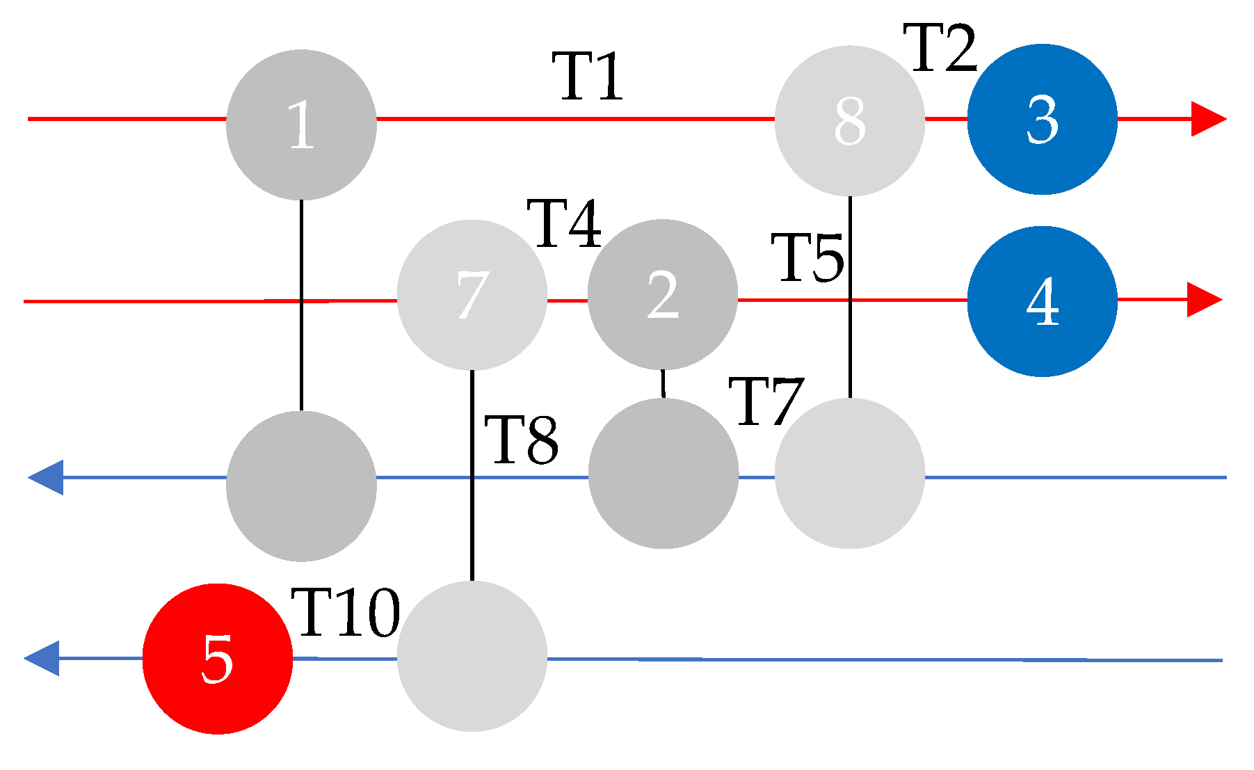
3.3. Determination of Critical Points

In the next step, critical operating points for each design proposal are identified using the different strategies for the identification of candidates for critical points and the set covering algorithm introduced by Pintarič and Kravanja [44]. The determination of critical operating points has been implemented in a methodology for synthesis of HENs with large numbers of uncertain parameters [45]. However, it has not yet been implemented in a retrofitting framework. The main difference in a retrofitting framework is that besides the investment cost of new HEXs, investment in existing equipment can also be considered, e.g., heat transfer enhancement or an increase of the area of existing HEXs, as well as structural changes, such as resequencing and repiping of existing HEXs. However, structurally, problems (5) and (6) are similar for a HEN synthesis and a HEN retrofitting problem.

It is worth mentioning that for the critical point analysis, each design proposal (which is present in the reduced superstructure) is considered individually, i.e., for each design proposal, this step yields an individual set of critical points. To allow a fast evaluation of the different design proposals, the different strategies for the identification of candidates for critical points and the set covering algorithm proposed in [44] were automated in this work in order to be applicable to a superstructure-based approach and industrial applications (see Supplementary Material).

3.4. Multi-Period Design Problem for Reduced Superstructure

With all critical points obtained, the multi-period design problem for the reduced superstructure and the representative operating points can be formulated. This problem is very similar to problem (5), with the exception that each design proposal $\mathrm{p}\in \mathrm{P}$ may include a not generalizable number of individual equality constraints $\mathrm{i}\in {\mathrm{I}}_{\mathrm{p}}$, inequality constraints $\mathrm{j}\in {\mathrm{J}}_{\mathrm{p}}$, and design constraints/variables $\mathrm{d}\in \mathrm{D}{\mathrm{V}}_{\mathrm{p}}$ as well as an individual set of critical points $\mathrm{c}\in \mathrm{C}{\mathrm{P}}_{\mathrm{p}}$, which results in an individual set of operating points $\mathrm{o}{\mathrm{p}}_{\mathrm{p}}\in \left(\mathrm{S}\cup \mathrm{C}{\mathrm{P}}_{\mathrm{p}}\right)$ at which the set of constraints of the respective design proposal must be satisfied. Therefore, problem (5) is reformulated:

$$\begin{array}{l}\min \mathrm{TAC}={\displaystyle {\displaystyle \sum }_{\mathrm{p}\in \mathrm{P}}}{\mathrm{y}}_{\mathrm{p}}\ast \left\{{\displaystyle {\displaystyle \sum }_{\mathrm{s}\in \mathrm{S}}}\left[{\mathrm{w}}_{\mathrm{s}}{\ast \mathrm{c}}_{\mathrm{operating},\mathrm{s},\mathrm{p}}\right]+{\mathrm{c}}_{\mathrm{investment},\mathrm{p}}\ast \mathrm{CRF}\right\}\\ \mathrm{s}.\mathrm{t}.\\ \begin{array}{l}{\mathrm{y}}_{\mathrm{p}}{\ast \mathrm{h}}_{\mathrm{i}}\left(\mathrm{x},\mathrm{z},\mathrm{d},{\mathsf{\theta }}_{\mathrm{op},\mathrm{p}}\right)=0;\mathrm{i}\in {\mathrm{I}}_{\mathrm{p}}\\ {\mathrm{y}}_{\mathrm{p}}{\ast \mathrm{g}}_{\mathrm{j}}\left(\mathrm{x},\mathrm{z},\mathrm{d},{\mathsf{\theta }}_{\mathrm{op},\mathrm{p}}\right)\le 0;\mathrm{j}\in {\mathrm{J}}_{\mathrm{p}}\\ {\mathrm{y}}_{\mathrm{p}}\ast \left[{\mathrm{g}}_{\mathrm{d}}\left(\mathrm{x},\mathrm{z},{\mathsf{\theta }}_{\mathrm{op},\mathrm{p}}\right)-\left({\mathrm{d}}_{\mathrm{existing}}+\mathrm{d}\right)\right] \le 0;\mathrm{d}\in {\mathrm{DV}}_{\mathrm{p}}\\ \mathrm{d}\ge 0\\ \mathrm{x},\mathrm{z},\mathrm{d},{\mathsf{\theta }}_{\mathrm{op},\mathrm{p}}\in \mathrm{R},{ \mathsf{\theta }}_{\mathrm{L}}\le {\mathsf{\theta }}_{\mathrm{op},\mathrm{p}}\le {\mathsf{\theta }}_{\mathrm{U}}\end{array}\}{\mathrm{op}}_{\mathrm{p}}\in \left(\mathrm{S}\cup {\mathrm{CP}}_{\mathrm{p}}\right)\\ {\displaystyle {\displaystyle \sum }_{\mathrm{p}\in \mathrm{P}}}{\mathrm{y}}_{\mathrm{p}}=1\\ {\mathrm{y}}_{\mathrm{p}}\in \left\{0,1\right\};\mathrm{p}\in \mathrm{P}.\end{array}$$

(7)

In problem (7), the set of individual design proposals of the reduced superstructure is represented by $\mathrm{p}\in \mathrm{P}$. Each design proposal is expressed via a binary variable ${\mathrm{y}}_{\mathrm{p}}$ and one and only one of these binary variables is forced to be 1, which will be the design proposal, which performs most cost efficiently at the representative operating points (and critical operating points). Instead of solving problem (7) simultaneously, it may also be solved proposal-wise, setting one ${\mathrm{y}}_{\mathrm{p}}$ to 1 and eventually comparing the TAC of all proposals to identify the most cost-efficient proposal of the reduced superstructure. In this context, it should be noted that all costs that can be associated with the respective retrofit design proposal must be included in the respective cost functions ${\mathrm{c}}_{\mathrm{operating},\mathrm{p}}$ and ${\mathrm{c}}_{\mathrm{investment},\mathrm{p}}$. This is especially important for retrofitting projects of industrial HENs, which are often very interconnected, and which may cause increased cost in other operational units.

3.5. Feasibility Check

In a final step, the feasibility is checked by means of the methodologies presented in Section 3.2. This step is necessary to ensure that all critical points have been identified (i.e., the set of critical points is complete). As outlined in Section 2.1, the previously derived HEX design characteristics are included, i.e., design constraints and solution obtained by solving the multi-period design problem. Since including design characteristics is likely to increase the complexity of the problem, solutions obtained by the methodologies presented in Section 3.2 should be analyzed and it is advisable to compare the achieved results of different methodologies to reduce the probability of failures. If feasibility for the respective design cannot be guaranteed, the result of the feasibility check can provide useful insights. Besides the flexibility index, the feasibility check provides a point in the space of the uncertain parameters, which limits the flexibility. The vector between this point and the average operating point (see Figure 1) can be used to generate candidates of critical points, which can be added to the multi-period design problem. If the newly generated design is feasible, the critical point has been successfully identified; otherwise, the new flexibility limit is analyzed, and the step is repeated until a feasible design is obtained.

4. Illustrative Example

The methodology described in Section 3 is illustrated using a four-stream example. The example was adapted from Lal et al. [34] with some modifications for demonstration purposes and was used as an initial network in a retrofitting process. In Figure 3, the initial network, the average stream data, and six different retrofit proposals are presented. These retrofit proposals are partly inspired by design proposals obtained by applying the Bridge analysis methodology presented in [34]. The main objective of the different retrofit proposals was to reduce the utility consumption in the heaters of the HEN.

Table 1. Hot utility demand for the initial heat exchanger network (HEN) and the different retrofit proposals as well as the potential savings for average operating conditions.

Proposal Number	Hot Utility Demand [kW] (at Average Conditions)	Hot Utility Savings [kW] (at Average Conditions)
Initial	2700	-
1)	1450	1250
2)	1900	800
3)	2000	700
4)	2000	700
5)	1450	1250
MER)	750	1950

shows the hot utility demand of the initial network as well as the hot utility demand and the hot utility savings of the six retrofit proposals.

The initial network consists of two process-to-process HEX and four utility HEXs. In

Table 2. Design characteristics of the initial network.

HEX	UA Value [kW/°C]	A [m2]
1	33.68	64.4
2	12.71	24.3

, the design characteristics of the existing process-to-process HEX are listed. For simplicity, it was assumed that the utility HEXs are not limited by size, i.e., any possible duty can be satisfied. For process-to-process HEX, a constant overall heat transfer coefficient (i.e., U-value) of 0.523 kW/(m² °C) was assumed.

4.1. Structural Feasibility Assessment

The proposed retrofit designs can be considered as different pathways in a superstructure, and in a next step, the structural feasibility of the different proposals was evaluated. For the evaluation, variations in the four inlet temperatures and heat capacity flow rates were assumed. The variations are shown in

Table 3. Variations of the average stream data.

Stream	ΔT+ [°C]	ΔT− [°C]	ΔFcp+ [kW/°C]	ΔFcp− [kW/°C]
H1	5	10	5	5
H2	10	10	5	5
C1	1	1	0.8	0.8
C2	25	20	2	2

.

The structural feasibility was evaluated by calculating the flexibility index using the active set approach developed by Floudas and Grossman [39]. Since all constraints $\mathrm{i}\in \mathrm{I}$ and $\mathrm{j}\in \mathrm{J}$ (see Section 2.1) are linear, the active set approach guarantees the globality of the solution [39]. In

Table 4. Results of the structural feasibility assessment of the different retrofit proposals.

Proposal Number	Structural Flexibility Index
1)	1.47
2)	1.47
3)	1.0
4)	1.0
5)	0.07
MER)	1.18

, the structural flexibility index for each retrofit proposal is listed.

The flexibility analysis revealed that retrofit proposal 5 is structurally infeasible, i.e., the structural flexibility index is smaller than 1 (see Table 4), meaning that for some operating points within the uncertainty span, the target temperature of at least one stream cannot be reached. This retrofit proposal was therefore removed from the initial superstructure of retrofit proposals, yielding a reduced superstructure.

4.2. Economic Data and Identification of Critical Points

In order to identify the critical points of the different retrofit design proposals, design variables were defined. These design variables could be modified in order to achieve feasibility for the entire range of operating conditions. It was assumed that the area of the two existing units could be increased while new units could be designed freely. Furthermore, the structure of the objective function of the overall design problem was specified. All in all, the total annualized cost (TAC) of the design should be minimized. Consequently, different cost functions were specified:

• Investment cost for a new HEX: $\mathrm{Inv}.\cos {\mathrm{t}}_{\mathrm{new}}$;
• Investment cost for increasing an existing HEX: $\mathrm{Inv}.\cos {\mathrm{t}}_{\mathrm{increase}}$;
• Operational cost for utility cooling: ${\mathrm{p}}_{\mathrm{CU}}$; and
• Operational cost for utility heating: ${\mathrm{p}}_{\mathrm{HU}}$.

Additionally, representative operating points $\mathrm{s}\in \mathrm{S}$, their normalized duration factor ${\mathrm{w}}_{\mathrm{s}}$, the capital recovery factor $\mathrm{CRF}$, and the annual operating time ${\mathrm{t}}_{\mathrm{operating}}$ were specified, in order to achieve cost efficiency for the entire operating period. The structure of the objective function for the retrofit design proposals is given in Equation (8):

$$\min \mathrm{TAC}={\displaystyle {\displaystyle \sum }_{\mathrm{s}\in \mathrm{S}}}\left[{\mathrm{w}}_{\mathrm{s}}\left({\mathrm{p}}_{\mathrm{CU}}{\mathrm{Q}}_{\mathrm{CU},\mathrm{s}}+{\mathrm{p}}_{\mathrm{HU}}{\mathrm{Q}}_{\mathrm{HU},\mathrm{s}}\right)\right]{\ast \mathrm{t}}_{\mathrm{operating}}+\left(\mathrm{Inv}.{\cos \mathrm{t}}_{\mathrm{increase}}+\mathrm{Inv}.{\cos \mathrm{t}}_{\mathrm{new}}\right)\ast \mathrm{CRF}.$$

(8)

As mentioned in Section 2.2, the cost function, which is minimized in problem (6) to identify critical points, does not include the operating cost of the representative operating points. The cost function that was used for determining the critical points is given in Equation (9):

$$\min \mathrm{C}=\left({\mathrm{p}}_{\mathrm{CU}}{\mathrm{Q}}_{\mathrm{CU}}+{\mathrm{p}}_{\mathrm{HU}}{\mathrm{Q}}_{\mathrm{HU}}\right){\ast \mathrm{t}}_{\mathrm{operating}}+\left(\mathrm{Inv}.{\cos \mathrm{t}}_{\mathrm{increase}}+\mathrm{Inv}.{\cos \mathrm{t}}_{\mathrm{new}}\right)\ast \mathrm{CRF}.$$

(9)

For simplicity, it was assumed that the increase of the two existing HEX units could be described by the same cost function. The cost for increasing a HEX in € is given in Equation (10) (A in m²):

$$\mathrm{Inv}.{\cos \mathrm{t}}_{\mathrm{increase}}=4000+2000{\ast \mathrm{A}}_{\mathrm{increase}}.$$

(10)

For new HEX units, it was also assumed that the same cost function is applicable for all possible new HEX units. The cost of a new HEX in € is given in Equation (11) (A in m²):

$$\mathrm{Inv}.{\cos \mathrm{t}}_{\mathrm{new}}=40,000+2000{\ast \mathrm{A}}_{\mathrm{HEX}}.$$

(11)

A capital recovery factor of 0.1 (e.g., 15 years lifetime and an interest rate of 7%) and an annual operating time of 8200 h were assumed. Furthermore, for the operating cost, the data in

Table 5. Cost data for operational cooling and heating.

Utility	Price [€/MWh]
Cooling (${\mathrm{p}}_{\mathrm{C}\mathrm{U}}$)	1.7 × 10−3
Heating (${\mathrm{p}}_{\mathrm{H}\mathrm{U}}$):	15

were used. It was further assumed that no additional costs are associated with the retrofit proposals.

For each of the five retrofit design proposals, which together constitute the reduced superstructure, one set of critical points was identified. These sets of critical points are listed in

Table A5. Sets of critical points for the different design proposal of the reduced superstructure.

Proposal Number	Critical Points (Read as Follows) [Tin,H1, Tin,H2, Tin,C1, Tin,C2, FcpH1, FcpH2, FcpC1, FcpC2] with T in [°C] and Fcp in [kW/°C]
1)	[240.0, 190.0, 21.0, 120.0, 10.0, 20.0, 20.8, 32.0]
	[255.0, 210.0, 19.0, 120.0, 10.0, 30.0, 20.8, 32.0]
	[240.0, 190.0, 19.0, 120.0, 10.0, 20.0, 20.8, 32.0]
2)	[240.0, 190.0, 19.0, 120.0, 10.0, 20.0, 20.8, 32.0]
	[240.0, 190.0, 19.0, 120.0, 20.0, 20.0, 20.8, 32.0]
	[255.0, 190.0, 19.0, 165.0, 20.0, 20.0, 19.2, 28.0]
	[255.0, 190.0, 19.0, 165.0, 0, 20.0, 20.8, 28.0]
3)	[240.0, 190.0, 21.0, 120.0, 10.0, 20.0, 20.8, 28.0]
	[240.0, 190.0, 19.0, 120.0, 10.0, 20.0, 20.8, 28.0]
	[255.0, 190.0, 0, 120.0, 20.0, 20.0, 20.8, 28.0]
4)	[240.0, 190.0, 21.0, 120.0, 20.0, 20.0, 20.8, 32.0]
	[240.0, 190.0, 19.0, 0, 10.0, 20.0, 20.8, 0]
	[255.0, 190.0, 0, 165.0, 20.0, 20.0, 19.2, 28.0]
MER)	[255.0, 190.0, 21.0, 165.0, 20.0, 30.0, 19.2, 28.0]
	[255.0, 190.0, 19.0, 120.0, 10.0, 20.0, 20.8, 32.0]
	[240.0, 190.0, 21.0, 120.0, 20.0, 20.0, 20.8, 32.0]
	[240.0, 210.0, 21.0, 120.0, 10.0, 30.0, 19.2, 32.0]
	[255.0, 210.0, 21.0, 165.0, 20.0, 30.0, 19.2, 28.0]
	[240.0, 190.0, 21.0, 120.0, 20.0, 30.0, 20.8, 32.0]
	[240.0, 210.0, 21.0, 120.0, 20.0, 30.0, 19.2, 32.0]
	[240.0, 190.0, 19.0, 120.0, 10.0, 20.0, 20.8, 32.0]

in Appendix B. The sets of critical points listed in Table A5 are complete, i.e., the designs based on these sets were proven to be feasible by means of flexibility analysis (see Section 4.3). To avoid numerical difficulties, the logarithmic mean temperature difference in the design constraints of the HEXs was approximated using Paterson’s approximation (see, e.g., [47]). As the determination of the critical points was connected to difficulties that were neither reported in the literature nor have been experienced when the results of the available literature examples of critical point analysis of HENs (see [44,45]) were reproduced, a description and a discussion on the determination of the critical points can be found in Appendix A. In this context, modifications on the existing methodologies were suggested to be able to determine critical points for more complex HEN structures but also for retrofit studies of HENs. For more information, see Appendix A.

4.3. Solution of the Multi-Period Design Problem and Final Feasibility Check

In the final step, the multi-period design problem was solved. In order to calculate the TAC of the different design proposals, representative operating points and their respective normalized duration factors were defined. For the illustrative example, 11 representative operating points were assumed. Furthermore, it was assumed that each operating point had the same normalized duration factor. The different representative operating points and their normalized duration factors are given in

Table A4. Representative operating points for the illustrative example.

Tin,H1 [°C]	Tin,H2 [°C]	Tin,HC1 [°C]	Tin,C2 [°C]	FcpH1 [kW/°C]	FcpH2 [kW/°C]	FcpC1 [kW/°C]	FcpC2 [kW/°C]	Ws [-]
243.65	208.10	19.59	155.49	15.44	23.23	20.14	28.60	1/11
249.72	202.83	20.29	156.26	16.14	21.22	19.87	29.51	1/11
246.41	202.73	20.34	162.06	16.50	28.27	20.49	29.59	1/11
248.81	194.63	20.04	133.91	16.40	25.15	20.23	31.24	1/11
249.82	202.35	20.76	136.65	12.00	27.33	19.72	31.40	1/11
247.16	200.40	19.21	124.26	14.96	25.44	19.88	30.61	1/11
248.18	200.50	20.56	158.58	19.83	24.80	20.51	28.78	1/11
242.30	206.05	19.89	157.40	11.83	22.99	19.61	30.97	1/11
244.50	207.36	19.13	160.11	14.09	25.36	19.99	30.75	1/11
248.71	204.38	20.02	140.01	13.03	20.93	20.18	30.28	1/11
253.53	191.07	19.39	127.44	12.99	27.18	20.29	30.82	1/11

in Appendix B. As can be seen in Table A4, extreme values (which can be calculated with the values given in Table 3) were not considered as representative operating points since these values represent extreme situations, which are usually not representative for longer operating periods.

To reduce the computational complexity, the multi-period design problem was solved individually for each retrofit proposal. The problems were solved using the global solver BARON.

Table 6. Total annualized cost, annual net savings, and flexibility index of the different retrofit design proposals in the reduced superstructure.

Proposal Number	Total Annualized Cost [€/y]	Net Savings [€/y]	Flexibility Index [-]
1)	228,000	86,600	1.00
2)	237,300	77,300	1.19
3)	250,000	64,600	1.00
4)	262,900	51,700	1.00
MER)	223,100	91,500	1.00

shows the TAC for the proposals in the reduced superstructure, the annual net savings (difference between the annual operating cost of the initial HEN and the TAC of the proposals), and the flexibility index. The annual operating cost of the initial HEN was used as a benchmark for the TAC of the different retrofit proposals and was calculated considering the cost data presented in Section 4.2. The annual operating cost of the initial network is 314,600 €/y. Additionally, the derived design values of the process-to-process HEXs of the different retrofit design proposals are shown in

Table A6. Design characteristics for design proposal 1.

HEX	ΔUA [kW/°C]	ΔA [m2]
1	13.58	25.97
2	1.02	1.95
7	77.81	148.77
8	9.94	19.01

,

Table A7. Design characteristics for design proposal 2.

HEX	ΔUA [kW/°C]	ΔA [m2]
1	0.0	0.0
2	26.5	50.67
7	26.59	50.84
8	19.35	37.0

,

Table A8. Design characteristics for design proposal 3.

HEX	ΔUA [kW/°C]	ΔA [m2]
1	74.87	143.16
2	39.71	75.93
7	57.59	110.11

,

Table A9. Design characteristics for design proposal 4.

HEX	ΔUA [kW/°C]	ΔA [m2]
1	74.87	143.16
2	20.04	38.32
7	24.69	47.21

and

Table A10. Design characteristics for design proposal MER.

HEX	ΔUA [kW/°C]	ΔA [m2]
1	26.71	51.07
2	103.96	198.78
7	33.22	63.51
8	9.57	18.30
9	89.36	170.85

in Appendix B. The results in Table 6 indicate that proposal MER is the most cost efficient.

The flexibility index was calculated using the active set approach developed by Floudas and Grossman [39] and the results were verified by searching for the minimum direction matrix using simulated annealing as it is reported in [40]. In contrast to [40], the subproblem to find the maximum value for δ (maximum feasible variation of the uncertain parameters) in a given direction was obtained by utilizing BARON. The parameters that were used for the simulated annealing algorithm are shown in

Table A11. Parameters for simulated annealing algorithm.

Parameter	Value
Initial temperature	10 K
Final temperature	2 × 10−20 K
Annealing of temperature	0.974*T
Stop criterion	No improvement after 2000 iterations

in Appendix B.

Introducing different representative operating points to the problem increases the problem size and complexity, which may cause longer CPU times to guarantee the globality of the obtained solution. The solutions presented above were obtained on an Intel i7-6600 2.6 GHz processor with 16.0 GB RAM in 1800 s. It is worth mentioning, that globality (within default EpsA range of BARON: 1e-6) could be achieved in the case of proposals 2, 3, and 4. However, it should be mentioned that the optimality gap for proposal 1 was less than 500 €/y while the largest remaining optimality gap was 37,000 €/y in case of proposal MER. Although the remaining optimality gap of the proposal MER is considerable in comparison to the possible savings, the found local solution was considered satisfactory as it indicates that proposal MER is the most cost efficient.

4.4. Discussion of the Results of the Illustrative Example

As mentioned previously, a discussion around the determination of the set of critical points for the different retrofit proposals of the illustrative example can be found in Appendix A.

Based on the results presented in Table 6, the proposal MER performs the most cost efficiently. This, however, relates to the used cost functions. Different cost functions will certainly lead to different results and another proposal may be most cost efficient. The influence of the cost functions can be illustrated by a comparison of the solutions of proposals 1 and MER. An analysis of the results of the multi-period design problem of proposals 1 and MER revealed that the TAC of proposal 1 consists of 23% annualized capital cost (and 77% operating cost) while the TAC of proposal MER consists of 56% annualized capital cost (and 44% operating cost). Thus, the used cost functions favor design proposals that allow more utilization of the HEX surface area. However, if the cost for the area is increased (e.g., increased parameters in investment cost functions), it can be assumed that design proposals that allow more utilization of utilities will be more cost efficient.

From Table 6, it can be seen that design proposal 2 has a significantly higher flexibility index than 1, which indicates overdesign of the HEX units. This overdesign results from the consideration of the chosen representative operating points. When the multi-period design problem for proposal 2 was solved considering only the identified set of critical points (and discard all operating cost), the flexibility index of the achieved design was calculated as 1. To check the influence of the representative operating periods and thereby the completeness of the identified sets of critical points, similar calculations were also made for the other design proposals in the reduced superstructure and the results are shown in

Table 7. Total annualized (capital) cost and flexibility index of the different retrofit design proposals in the reduced superstructure without considering the representative operating points.

Proposal Number	Total Annualized (Capital) Cost [€/y]	Flexibility Index [-]
1)	19,600	1.00
2)	19,600	1.00
3)	37,200	1.00
4)	37,200	1.00
MER)	95,600	1.00

. The results in Table 7 indicate that the sets of critical points shown in Table A5 are complete as it was possible to achieve feasible design characteristics (flexibility index is 1) respecting only the sets of critical points. As all operating costs were discarded, the objective function of these design problems represented only the total annualized capital cost of a certain design.

5. Conclusions

In this work, a novel framework for retrofitting multi-period HENs was developed and presented. The proposed framework divides the retrofit design process into five sub-steps, which allows for the combining of the beneficial designer interaction of graphical approaches (e.g., Pinch based) at an early stage in the design process with the efficiency of mathematical programming to derive flexible and cost-efficient retrofit measures. In this context, inefficient trial and error procedures are avoided. Additionally, by means of splitting the design process in five different sub-steps, the complexity of the sub-problems is decreased compared to the overall problem.

The proposed framework utilizes the designer interaction of graphical approaches to derive different design proposals, which can be very beneficial for large and complex HENs usually found in industrial heat recovery systems. Well-proven, single-period retrofit design methods, such as Bridge analysis, but also “experience-based” retrofit design proposals may be employed. As the single-period character of graphical retrofitting methodologies does not ensure the flexibility and cost-efficiency of the generated proposals for the entire operating period, different mathematical evaluation strategies are incorporated in the proposed framework. By means of structural feasibility assessment based on the calculation of the flexibility index, structurally infeasible design proposals can be identified and discarded from further analysis. Additionally, critical point analysis was suggested to identify those operating points within the uncertainty span that determine necessary overdesign of the HEXs to ensure feasibility of the HEN retrofit proposals for the entire operating range. In order to identify the most cost-efficient proposal, a multi-period MI(N)LP optimization problem was formulated, which considerers the identified critical points (for feasibility) as well as representative operating points (for cost-efficiency). A final feasibility check was suggested to ensure that the complete set of critical points has been identified.

The determination of critical points based on [44] was automated and the achieved results were discussed. Compared to the available literature examples, the HEN examples included in this study are more complex, which caused difficulties when determining critical points. Modifications of the existing methodologies (see Appendix A) were suggested in order to identify the complete set of critical points for the HEN retrofit example presented in this study. It is worth mentioning that by means of the above-mentioned final feasibility check, an incomplete set of critical points is recognized. Additionally, by means of the obtained results of the final feasibility check, the missing critical point(s) can be identified to be included in the multi-period MI(N)LP design problem.

The framework presented in this paper yields opportunities to increase heat recovery in applications operating at multiple periods, e.g., industrial applications. As decarbonization of industry is essential to limit the increase of the global average temperature well below 2 °C, systematic approaches to successfully retrofit industrial heat recovery systems are in demand more than ever. In comparison to existing approaches for retrofitting multi-period HENs, the presented framework splits the design process in five different sub-steps, which decreases the complexity of the sub-problems. The decreased complexity can be the decisive factor for a successful retrofit project when large and complex industrial applications are addressed. The novel contributions of this paper are summarized in the following list:

• Development of a novel framework to achieve flexible and cost-efficient retrofit measures for HENs operating at multiple periods;
• Implementation of critical point analysis in a retrofitting framework to achieve flexible retrofit solutions of HENs;
• Possibility to employ well-proven, single-period retrofit design methods, e.g., advanced composite curves, Bridge analysis, etc., but also “experience-based” retrofit design proposals in a framework that guarantees flexibility and cost efficiency (with respect to investment and operating cost) for the entire operating period;
• Possibility to compare design proposals of different single-period retrofit design methods in a superstructure-based mathematical program ensuring flexibility and cost efficiency with respect to investment and operating cost;
• Automatization of the KKT-formulation, the two-level formulation, and the set-covering algorithm initially suggested by Pintarič and Kravanja [44] to identify critical points of different design proposals (see Supplementary Material); and
• Extension of the set covering algorithm suggested by Pintarič and Kravanja [44] in order to handle more complex network structures (see Appendix A).

References

1. Linnhoff, B.; Hindmarsh, E. The pinch design method for heat exchanger networks. Chem. Eng. Sci. 1983, 38, 745–763. [Google Scholar] [CrossRef]
2. Floudas, C.A.; Ciric, A.R.; Grossmann, I.E. Automatic synthesis of optimum heat exchanger network configurations. AIChE J. 1986, 32, 276–290. [Google Scholar] [CrossRef]
3. Yee, T.F.; Grossmann, I.E. Simultaneous optimization models for heat integration. II. Heat exchanger network synthesis. Comput. Chem. Eng. 1990, 14, 1165–1184. [Google Scholar] [CrossRef]
4. Jiang, N.; Bao, S.; Gao, Z. Heat Exchanger Network Integration Using Diverse Pinch Point and Mathematical Programming. Chem. Eng. Technol. 2011, 34, 985–990. [Google Scholar] [CrossRef]
5. Axelsson, E.; Olsson, M.R.; Berntsson, T. Heat integration opportunities in average Scandinavian kraft pulp mills: Pinch analyses of model mills. Nord. Pulp Pap. Res. J. 2006, 21, 466–475. [Google Scholar] [CrossRef]
6. Bengtsson, C.; Nordman, R.; Berntsson, T. Utilization of excess heat in the pulp and paper industry—A case study of technical and economic opportunities. Appl. Therm. Eng. 2002, 22, 1069–1081. [Google Scholar] [CrossRef]
7. Escobar, M.; Trierweiler, J.O. Optimal heat exchanger network synthesis: A case study comparison. Appl. Therm. Eng. 2013, 51, 801–826. [Google Scholar] [CrossRef]
8. Persson, J.; Berntsson, T. Influence of seasonal variations on energy-saving opportunities in a pulp mill. Energy 2009, 34, 1705–1714. [Google Scholar] [CrossRef]
9. Kang, L.; Liu, Y. Synthesis of flexible heat exchanger networks: A review. Chin. J. Chem. Eng. 2019, 27, 1485–1497. [Google Scholar] [CrossRef]
10. Kotjabasakis, E.; Linnhoff, B. Sensitivity tables for the design of flexible processes (1)—How much contingency in heat exchanger networks is cost-effective? Chem. Eng. Res. Des. 1986, 64, 197–211. [Google Scholar]
11. Hafizan, A.M.; Klemeš, J.J.; Alwi, S.R.W.; Manan, Z.A.; Hamid, M.K.A. Temperature disturbance management in a heat exchanger network for maximum energy recovery considering economic analysis. Energies 2019, 12, 594. [Google Scholar] [CrossRef] [Green Version]
12. Linnhoff, B.; Vredeveld, D.R. Pinch Technology Has Come of Age. Chem. Eng. Prog. 1984, 80, 33–40. [Google Scholar]
13. Floudas, C.A.; Grossmann, I.E. Synthesis of flexible heat exchanger networks for multiperiod operation. Comput. Chem. Eng. 1986, 10, 153–168. [Google Scholar] [CrossRef]
14. Floudas, C.A.; Grossmann, I.E. Automatic generation of multiperiod heat exchanger network configurations. Comput. Chem. Eng. 1987, 11, 123–142. [Google Scholar] [CrossRef]
15. Floudas, C.A.; Grossmann, I.E. Synthesis of flexible heat exchanger networks with uncertain flowrates and temperatures. Comput. Chem. Eng. 1987, 11, 319–336. [Google Scholar] [CrossRef]
16. Aaltola, J. Simultaneous synthesis of flexible heat exchanger network. Appl. Therm. Eng. 2002, 22, 907–918. [Google Scholar] [CrossRef]
17. Verheyen, W.; Zhang, N. Design of flexible heat exchanger network for multi-period operation. Chem. Eng. Sci. 2006, 61, 7730–7753. [Google Scholar] [CrossRef]
18. Short, M.; Isafiade, A.J.; Fraser, D.M.; Kravanja, Z. Two-step hybrid approach for the synthesis of multi-period heat exchanger networks with detailed exchanger design. Appl. Therm. Eng. 2016, 105, 807–821. [Google Scholar] [CrossRef]
19. Tveit, T.M.; Aaltola, J.; Laukkanen, T.; Laihanen, M.; Fogelholm, C.J. A framework for local and regional energy system integration between industry and municipalities-Case study UPM-Kymmene Kaukas. Energy 2006, 31, 2162–2175. [Google Scholar] [CrossRef]
20. Lai, Y.Q.; Manan, Z.A.; Alwi, S.R.W. Simultaneous diagnosis and retrofit of heat exchanger network via individual process stream mapping. Energy 2018, 155, 1113–1128. [Google Scholar] [CrossRef]
21. Kamel, D.A.; Gadalla, M.A.; Abdelaziz, O.Y.; Labib, M.A.; Ashour, F.H. Temperature driving force (TDF) curves for heat exchanger network retrofit—A case study and implications. Energy 2017, 123, 283–295. [Google Scholar] [CrossRef]
22. Bonhivers, J.C.; Srinivasan, B.; Stuart, P.R. New analysis method to reduce the industrial energy requirements by heat-exchanger network retrofit: Part 1—Concepts. Appl. Therm. Eng. 2017, 119, 659–669. [Google Scholar] [CrossRef]
23. Ciric, A.R.; Floudas, C.A. A comprehensive optimization model of the heat exchanger network retrofit problem. Heat Recovery Syst. CHP 1990, 10, 407–422. [Google Scholar] [CrossRef]
24. Asante, N.D.K.; Zhu, X.X. An automated and interactive approach for heat exchanger network retrofit. Chem. Eng. Res. Des. 1997, 75, 349–360. [Google Scholar] [CrossRef]
25. Athier, G.; Floquet, P.; Pibouleau, L.; Domenech, S. A mixed method for retrofiting heat-exchanger networks. Comput. Chem. Eng. 1998. [Google Scholar] [CrossRef]
26. Smith, R.; Jobson, M.; Chen, L. Recent development in the retrofit of heat exchanger networks. Appl. Therm. Eng. 2010, 30, 2281–2289. [Google Scholar] [CrossRef] [Green Version]
27. Jiang, N.; Shelley, J.D.; Doyle, S.; Smith, R. Heat exchanger network retrofit with a fixed network structure. Appl. Energy 2014. [Google Scholar] [CrossRef]
28. Akpomiemie, M.O.; Smith, R. Retrofit of heat exchanger networks with heat transfer enhancement based on an area ratio approach. Appl. Energy 2016. [Google Scholar] [CrossRef]
29. Sreepathi, B.K.; Rangaiah, G.P. Review of Heat Exchanger Network Retrofitting Methodologies and Their Applications. Ind. Eng. Chem. Res. 2014, 53, 11205–11220. [Google Scholar] [CrossRef]
30. Persson, J.; Berntsson, T. Influence of short-term variations on energy-saving opportunities in a pulp mill. J. Clean. Prod. 2010, 18, 935–943. [Google Scholar] [CrossRef]
31. Kang, L.; Liu, Y. Retrofit of heat exchanger networks for multiperiod operations by matching heat transfer areas in reverse order. Ind. Eng. Chem. Res. 2014, 53, 4792–4804. [Google Scholar] [CrossRef]
32. Papalexandri, K.P.; Pistikopoulos, E.N. A Retrofit Design Model for Improving the Operability of Heat Exchanger Networks. In Energy Efficiency in Process Technology; Pilavachi, P.A., Ed.; Springer: Dordrecht, The Netherlands, 1993; pp. 915–928. [Google Scholar]
33. Nordman, R.; Berntsson, T. Use of advanced composite curves for assessing cost-effective HEN retrofit I: Theory and concepts. Appl. Therm. Eng. 2009, 29, 275–281. [Google Scholar] [CrossRef]
34. Lal, N.S.; Atkins, M.J.; Walmsley, T.G.; Walmsley, M.R.W.; Neale, J.R. Insightful heat exchanger network retrofit design using Monte Carlo simulation. Energy 2019, 181, 1129–1141. [Google Scholar] [CrossRef]
35. Langner, C.; Svensson, E.; Harvey, S. Combined Flexibility and Energy Analysis of Retrofit Actions for Heat Exchanger Networks. Chem. Eng. Trans. 2019, 76, 307–312. [Google Scholar] [CrossRef]
36. Marselle, D.F.; Morari, M.; Rudd, D.F. Design of resilient processing plants—II Design and control of energy management systems. Chem. Eng. Sci. 1982, 37, 259–270. [Google Scholar] [CrossRef]
37. Saboo, A.K.; Morari, M.; Woodcock, D.C. Design of resilient processing plants-VIII. A resilience index for heat exchanger networks. Chem. Eng. Sci. 1985, 40, 1553–1565. [Google Scholar] [CrossRef]
38. Swaney, R.E.; Grossmann, I.E. An index for operational flexibility in chemical process design. Part I: Formulation and Theory. AIChE J. 1985, 31, 621–630. [Google Scholar] [CrossRef]
39. Grossmann, I.E.; Floudas, C.A. Active constraint strategy for flexibility analysis in chemical processes. Comput. Chem. Eng. 1987, 11, 675–693. [Google Scholar] [CrossRef] [Green Version]
40. Li, J.; Du, J.; Zhao, Z.; Yao, P. Efficient Method for Flexibility Analysis of Large-Scale Nonconvex Heat Exchanger Networks. Ind. Eng. Chem. Res. 2015, 54, 10757–10767. [Google Scholar] [CrossRef]
41. Zhao, F.; Chen, X. Analytical and triangular solutions to operational flexibility analysis using quantifier elimination. AIChE J. 2018, 64, 3894–3911. [Google Scholar] [CrossRef]
42. Li, J.; Du, J.; Zhao, Z.; Yao, P. Structure and area optimization of flexible heat exchanger networks. Ind. Eng. Chem. Res. 2014, 53, 11779–11793. [Google Scholar] [CrossRef]
43. Pintarič, Z.N.; Kasaš, M.; Kravanja, Z. Sensitivity Analyses for Scenario Reduction in Flexible Flow Sheet Design with a Large Number of Uncertain Parameters. AIChE J. 2013, 59, 2862–2871. [Google Scholar] [CrossRef]
44. Pintarič, Z.N.; Kravanja, Z. Identification of critical points for the design and synthesis of flexible processes. Comput. Chem. Eng. 2008, 32, 1603–1624. [Google Scholar] [CrossRef]
45. Pintarič, Z.N.; Kravanja, Z. A methodology for the synthesis of heat exchanger networks having large numbers of uncertain parameters. Energy 2015, 92, 373–382. [Google Scholar] [CrossRef]
46. Kachacha, C.; Zoughaib, A.; Tran, C.T. A methodology for the flexibility assessment of site wide heat integration scenarios. Energy 2018, 154, 231–239. [Google Scholar] [CrossRef]
47. Pettersson, F. Heat exchanger network design using geometric mean temperature difference. Comput. Chem. Eng. 2008, 32, 1726–1734. [Google Scholar] [CrossRef]
Figure 1. (Hyper-)rectangle with respect to expected variations and maximum scaled (hyper-)rectangle inscribed within the feasible region in the space of the varying inlet temperatures of a heat exchanger network [38].
Energies 13 01472 g001
Figure 2. Retrofitting framework to achieve flexible and cost-efficient retrofit measures of heat exchanger networks (HENs).
Energies 13 01472 g002
Figure 3. Initial network with average stream data and six different retrofit proposals.
Energies 13 01472 g003