Nonlinear Finite Element Analysis-Based Flow Distribution and Heat Transfer Model ^†

Abstract

A new strategy for fast, approximate analyses of fluid flow and heat transfer is presented. It is based on Finite Element Analysis (FEA) and is intended for large yet structurally fairly simple heat transfer equipment commonly used in process and power industries (e.g., cross-flow tube bundle heat exchangers), which can be described using sets of interconnected 1-D meshes. The underlying steady-state model couples an FEA-based (linear) predictor step with a nonlinear corrector step, which results in the ability to handle both laminar and turbulent flows. There are no limitations in terms of the allowed temperature range other than those potentially stemming from the usage of fluid physical property computer libraries. Since the fluid flow submodel has already been discussed in the referenced conference paper, the present article focuses on the prediction of the tube side and the shell side temperature fields. A simple cross-flow tube bundle heat exchanger from the literature and a heat recovery hot water boiler in an existing combined heat and power plant, for which stream data are available from its operator, are evaluated to assess the performance of the model. To gain further insight, the results obtained using the model for the heat recovery hot water boiler are also compared to the values yielded by an industry-standard heat transfer equipment design software package. Although the presented strategy is still a “work in progress” and requires thorough validation, the results obtained thus far suggest it may be a promising research direction.

1. Introduction

During design, operation, and troubleshooting of various process and power equipment-containing tube bundles, it often is important to know the velocity and temperature fields in both the tube and the shell sides. These are obtained predominantly using Computational Fluid Dynamics (CFD) models and, therefore, articles covering a wide range of such applications are available. For example, Wei et al. [1] discussed a coupled CFD-Lagrange multipliers optimization method for flow distribution adjustments to prevent freezing of power generation natural draft cooling systems during winter operation. Chien et al. [2], on the other hand, presented a coupled CFD-surrogate-based optimization of flow distribution in a heat exchanger inlet header. Zhou et al. [3] focused on CFD investigation and optimization of a compact heat exchanger comprising a single row of tubes, and Łopata et al. [4] published an article covering the experimental investigation of flow distribution in a similar cross-flow heat exchanger, but with a tube bank consisting of elliptical tubes. CFD evaluation and optimization of solar collectors, commonly also using a single row of risers, were discussed, for instance, by García-Guendulain et al. [5], who aimed to improve the collector performance by changes of riser-to-header cross-sectional area and diameter ratios. Karvounis et al. [6] carried out a numerical and experimental study of the flow field in a forced circulation Z-type flat plate solar collector. Articles focusing on two-phase flow are also common. Li et al. [7] studied flow reversal in vertically inverted U-tube steam generators used in marine nuclear power plants, whereas Klenov and Noskov [8] investigated the effect of two-phase flow pattern in an inlet duct on flow distribution in the upper part of a trickle bed reactor. As for dispersion headers, which are often used in flue gas cleaning equipment, a CFD investigation of the impacts of inlet flow rate, hole diameter, and downstream distance on the flow distribution in an annular multi-hole header was presented by He et al. [9]. Other frequent research areas where the knowledge of flow distribution is critical are fuel cells and micro-channel heat exchangers. One might mention, e.g., the CFD and laser Doppler velocimetry investigation of flow distribution in a polymer electrolyte membrane fuel cell stack by Bürkle et al. [10], the CFD evaluation of pressure and flow distribution effects on the performance of polymer electrolyte membrane fuel cells by Heck et al. [11], or the CFD optimization of a liquid cooling system of a power inverter in an electric vehicle presented by Hur et al. [12]. Various studies involving liquid-cooled micro-channel heat sinks for electronics are quite common as well. See, e.g., the article by Li et al. [13] discussing the optimization of the micro-channel topology.

Studies not utilizing CFD are much less common and, typically, focus on evaluations of the respective equipment via physical experiments. To name just a few, one could mention the experimental investigation of flow distribution and its effect on the performance of a plate-fin heat exchanger by Zhu et al. [14], the study of two-phase refrigerant distribution in a finned-tube evaporator by Tang et al. [15], or the article by Quintanar et al. [16] covering natural circulation flow distribution in a multi-branch manifold. Micro-channel equipment was discussed, e.g., by Yih and Wang [17], who carried out an experimental investigation of the thermal-hydraulic performance of a micro-channel heat exchanger for waste heat recovery, or by Lugarini et al. [18], who focused on the evaluation of flow distribution uniformity in a comb-like micro-channel network. On the other end of the size spectrum are heat exchanger networks, in which Ishiyama and Pugh [19] studied thermo-hydraulic channeling in the individual parallel branches. In their paper, they also presented a model for prediction of flow distribution in the branches for the case when no flow control was implemented. Similarly, Novitsky et al. [20] discussed multilevel modeling and optimization of large-scale pipeline systems using specialized software tools. In these two studies, however, modelling of pressure drop was only done in a simplified manner. Korelstein [21], on the other hand, discussed mathematical properties of classical hydraulic network flow distribution problems which included pressure-dependent closure relations. An essentially identical problem can also be encountered when it comes to the design of water distribution networks. Still, proper inclusion of pressure drop in the respective models is rare because they generally focus on layout optimization while meeting the local water demands (see, for instance, the article by Cassiolato et al. [22], who proposed a Mixed-Integer Nonlinear Programming (MINLP) model for this purpose), identification of sources of contamination (as done, e.g., using a convolutional neural network by Sun et al. [23]), detection of leakage points (see, for example, the article by Fang et al. [24]), evaluation of the network performance and reliability (as discussed, e.g., in the Hanoi case study by Jeong and Kang [25]), etc.

To the best of the authors’ knowledge, there currently is no semi-accurate but fast Finite Element Analysis-based model of fluid flow other than [26] that would properly include the pressure drop. This model, however, does not consider heat transfer and, thus, is of limited practical value to the designers of process and power equipment. Consequently, CFD models, because of their significant computational cost, are being employed for evaluations of fluid flow distribution and heat transfer only if absolutely necessary. As a result, the corresponding temperature fields, which, to a large degree, depend on mass flow rates through individual tubes, are also unknown. This may not pose significant problems if thermal stress is relatively even throughout the tube bundle in question. Nonetheless, mechanical failures of bundles, stemming from improper design procedures which a priori assume uniform flow distribution, are not uncommon when it comes to heat exchangers featuring large changes in stream temperatures. The present paper, therefore, introduces a significantly extended version of the flow-only, adiabatic model discussed in [26]. This includes heat transfer between the fluids in the tube and the shell sides of a cross-flow tube bank heat exchanger (e.g., an economizer) as well as various other improvements. Shell-side flow was modelled as unidirectional. As test cases, a simple cross-flow tube bundle heat exchanger from the literature and an existing heat recovery hot water boiler, for which the necessary data had been provided by its operator, were considered. These were compared to the results obtained using the present model and, to gain further insight, also to the data from an industry-standard heat exchanger design software package. A good agreement among the data sets was observed.

2. Materials and Methods

The original model discussed in [26] assumed adiabatic flow, that is, no heat transfer was allowed on the walls of the parallel flow channels in the distribution system. The model was shown in the same article to provide data with relative errors of at most 4% compared to detailed transient CFD simulations even in the case of highly turbulent flows. Such accuracy was achievable due to the relative simplicity of the flow systems for which the respective model has been intended (e.g., tube bundles in heat recovery steam generators). The overall conclusion, therefore, was that, in terms of application in preliminary analyses of selected heat transfer equipment or for shape optimization of the mentioned equipment, the model was suitable for engineering practice.

Because of the nature of the model, its performance in case of laminar flow was a priori expected to be acceptable. Although several tests were carried out earlier even with low total mass flow rates to make sure this really was the case, no example was given in [26]. To remedy this, let us mention, for instance, one of the test flow distribution systems (see Figure 1) used in the original article and the respective laminar flow distribution data and relative errors. For convenience’s sake, parameters of the flow system are listed in

Table 1. Parameters of the flow distribution system used to obtain the laminar flow-related data shown in Figure 1.

Parameter	Value
headers (W × H × L)	55 × 55 × 280 mm
tube bundle	5 rows with 10 tubes each, tube layout: 60°
tubes	straight, inner diameter: 10 mm, length: 2000 mm
fluid	water, 0.5 kg s−1, 300 K
flow regime	laminar, average tube Re ≈ 1500

. The obtained mass flow rates are compared in Figure 2a, while Figure 2b shows the corresponding relative errors. It can be seen that the error values generally were in a ±1% band with only two of them being at around 1.2%. Relative errors obtained using other test flow systems were of similar magnitudes. Thus, one could conclude that, in the case of laminar flow, the accuracy was even better than when the flow was highly turbulent.

2.1. Inclusion of Heat Transfer into the Model

The main shortcoming of the original, flow-only version of the Finite Element Analysis (FEA)-based model was its inability to properly evaluate tube bundles in which heat transfer could not be neglected. Given the intended purpose of the model (that is, usage in engineering practice), this functionality had to be implemented.

Please note that heat transfer was not, strictly speaking, evaluated using FEA. However, the temperature fields in the tube side and the shell side were still obtained using a system of linear equations generated as shown in the following text, and this system was then solved in the usual manner. It was assumed that the temperature profile between two end nodes of an edge was continuous and was given by the mean temperatures on control volume cross-sections, which were perpendicular to the corresponding edge. The iterative solver then worked similarly to any other segregated solver. First, the fluid flow (FEA-based) submodel was solved under the assumption of a constant temperature field. Next, the heat transfer submodel was solved under the assumption of a constant velocity field. This was followed by the update of the fluid physical properties and other necessary post-iteration tasks, and then the fluid flow submodel was solved again. This iterative procedure was repeated until convergence was reached.

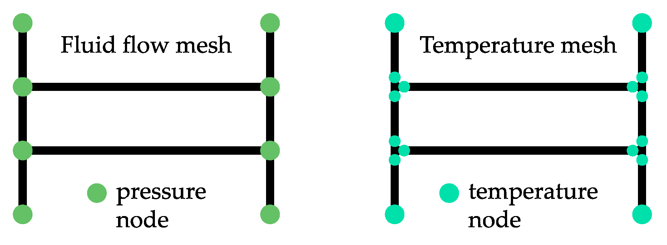
Even though the heat transfer submodel was not using FEA, the corresponding mesh on which the temperature field was calculated can be constructed in a similar manner. In the fluid flow mesh, the field to be calculated was described by total pressures in the nodes. The temperature field can be described analogously with the difference being that every edge had its own temperature in the node. Figure 3 shows the two meshes and the differences between meshes.

As mentioned before, the temperatures were calculated using a set of linear equations. From Figure 3 it is clear that a flow system consisting of n edges will feature 2n node temperatures and, therefore, 2n linear equations were required. There were three classes of temperature-related equations that were used in the model:

• Flow mixing and splitting,
• Heat transfer through channel walls, and
• Boundary conditions.

2.1.1. Flow Mixing and Splitting

When, in an arbitrary mesh node, streams q₁, q₂, …, q_m are mixed into a single stream j, we can write

$${\displaystyle \sum }_{q\in \left\{q_1,q_2,\dots ,q_m\right\}}{\dot{m}}_q{c}_{\mathrm{p},q}\left(T_j-T_q\right)=0.$$

(1)

Here, ${\dot{m}}_q$ denotes the mass flow rate of the qth stream, c_p,q the specific heat capacity, and T_j and T_q the corresponding stream temperatures. Each specific heat capacity should be taken as the mean value obtained for the corresponding temperature range [T_j, T_q].

If, on the other hand, a single stream j is split into streams r₁, r₂, …, r_n, the outflow temperature is the same for all these streams, and the respective n equations are

$$T_r=T_j, r\in \left\{r_1,r_2,\dots ,r_n\right\}.$$

(2)

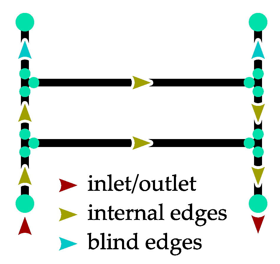
In some systems, there may be blind edges with zero mass flow rate. The temperatures in the nodes of these edges are calculated as if the edges were of the regular type featuring outflow (see also the schematic in Figure 4).

In a general case with streams q₁, q₂, …, q_m being mixed and then split into streams r₁, r₂, …, r_n, one will get one Equation (1) governing the resulting outflow temperature T_j and (n − 1) Equation (2), that is, (n − 1) identities for the remaining outflow temperatures. The total number of equations governing the mixing/splitting in the node will, therefore, be equal to number of outflow streams.

2.1.2. Heat Transfer through Channel Walls

Let us have two meshes representing the tube and the shell sides of a heat exchanger and focus on an arbitrary pair of adjacent control volumes representing a portion of the tube side (i.e., a tube segment) and the enclosing portion of the shell side (see Figure 5). Let ${\dot{m}}_{\mathrm{t}}$, c_p,t, T_t,1, and T_t,2 denote the tube side mass flow rate, mean specific heat capacity at constant pressure, and inlet and outlet temperatures and ${\dot{m}}_{\mathrm{s}}$, c_p,s, T_s,1, and T_s,2 the corresponding shell-side quantities.

Should, e.g., the hot fluid be placed in the shell side, then the overall heat balance could be written as

$${\dot{m}}_{\mathrm{t}}{c}_{\mathrm{p},\mathrm{t}}\left(T_{\mathrm{t},2}-T_{\mathrm{t},1}\right)={\dot{m}}_{\mathrm{s}}{c}_{\mathrm{p},\mathrm{s}}\left(T_{\mathrm{s},1}-T_{\mathrm{s},2}\right).$$

(3)

Let us for a moment assume that the temperature of the fluid in the shell-side control volume is constant and is equal to the shell-side inlet temperature, T_s,1. Let us also assume that the tube-side inlet temperature, T_t,1, is known. Additionally, let L denote the length of the tube-side mesh edge and U the cumulative overall heat transfer coefficient. The heat flux for a small portion of this edge having the length dx can then be expressed as

$$\mathrm{d}\dot{Q}={\dot{m}}_{\mathrm{t}}{c}_{\mathrm{p},\mathrm{t}}\left(T_{\mathrm{t}}\left(x+\mathrm{d}x\right)-T_{\mathrm{t}}\left(x\right)\right)=U\frac{\mathrm{d}x}{L}\left(T_{\mathrm{s},1}-T_{\mathrm{t}}\left(x\right)\right).$$

(4)

This can be modified, rearranged, and written in integral form,

$${{\displaystyle \int }}_{T_{\mathrm{t},1}}^{T_{\mathrm{t}}\left(x\right)}\frac{1}{T_{\mathrm{s},1}-T_{\mathrm{t}}\left(x\right)}\mathrm{d}{T}_{\mathrm{t}}\left(x\right)=\underset{0}{\overset{x}{{\displaystyle \int }}}\frac{U}{{\dot{m}}_{\mathrm{t}}{c}_{\mathrm{p},\mathrm{t}}L}\mathrm{d}x,$$

(5)

which yields

$$T_{\mathrm{t}}\left(x\right)=T_{\mathrm{s},1}+\left(T_{\mathrm{t},1}-T_{\mathrm{s},1}\right)\exp \left(-\frac{U}{{\dot{m}}_{\mathrm{t}}{c}_{\mathrm{p},\mathrm{t}}}\frac{x}{L}\right), x\in \left[0,L\right].$$

(6)

From Equation (6), we immediately see that the temperature at the end of the edge can be obtained using

$$T_{\mathrm{t},2}=T_{\mathrm{s},1}+\left(T_{\mathrm{t},1}-T_{\mathrm{s},1}\right)\exp \left(-\frac{U}{{\dot{m}}_{\mathrm{t}}{c}_{\mathrm{p},\mathrm{t}}}\right).$$

(7)

Equation (7) must be linearized for it to be used in a matrix solver. This is done in a straightforward manner by taking

$$C_U=\exp \left(-\frac{U}{{\dot{m}}_{\mathrm{t}}{c}_{\mathrm{p},\mathrm{t}}}\right)=\mathrm{const}.,$$

(8)

where the necessary cumulative overall heat transfer coefficient, U, is computed from the tube-side and shell-side heat transfer coefficients. These, in turn, are calculated using equations from literature (e.g., [28] in the case of plain tubes or [29] if the tubes are finned) depending on the actual bundle geometry and flow conditions. Additional information regarding validation of the commonly used empirical equations for estimation of heat transfer coefficient in the case of plain and serrated fins can be found, for instance, in [30]. One could also use the correlations from [31], which have been obtained via the machine learning technique. If U-shaped or helical fins of various types are employed, then the two-part article by Hofmann and Heimo [32,33] can be recommended to the reader. The final, linearized equation for a single edge, therefore, is

C_UT_t,1 − T_t,2 = (C_U − 1) T_s,1.

(9)

Considering the shell-side outlet temperature, for cross-flow with T_s,1 = const. on the entire inlet face of the control volume, we have

$$\mathrm{d}\dot{Q}=U\frac{\mathrm{d}x}{L}\left(T_{\mathrm{s},1}-T_{\mathrm{t}}\left(x\right)\right)={\dot{m}}_{\mathrm{s}}{c}_{\mathrm{p},\mathrm{s}}\frac{\mathrm{d}x}{L}\left(T_{\mathrm{s},1}-T_{\mathrm{s},2}\left(x\right)\right).$$

(10)

Just as before, this can be modified and rearranged to yield

$$T_{\mathrm{s},2}\left(x\right)=T_{\mathrm{s},1}+\frac{U}{{\dot{m}}_{\mathrm{s}}{c}_{\mathrm{p},\mathrm{s}}}\left(T_{\mathrm{s},1}-T_{\mathrm{t},1}\right)\exp \left(-\frac{U}{{\dot{m}}_{\mathrm{t}}{c}_{\mathrm{p},\mathrm{t}}}\frac{x}{L}\right), x\in \left[0,L\right].$$

(11)

The mean shell-side outlet temperature then is

$$T_{\mathrm{s},2}=\frac{1}{L}{{\displaystyle \int }}_0^L{T}_{\mathrm{s},2}\left(x\right)\mathrm{d}x=T_{\mathrm{s},1}+\frac{{\dot{m}}_{\mathrm{t}}{c}_{\mathrm{p},\mathrm{t}}}{{\dot{m}}_{\mathrm{s}}{c}_{\mathrm{p},\mathrm{s}}}\left(\exp \left(-\frac{U}{{\dot{m}}_{\mathrm{t}}{c}_{\mathrm{p},\mathrm{t}}}\right)-1\right)\left(T_{\mathrm{s},1}-T_{\mathrm{t},1}\right),$$

(12)

which corresponds to the shell-side outlet temperature obtained using the respective set of linear equations.

One could also simplify the model even further by using a one-dimensional shell-side mesh (i.e., a mesh such that each cross-section of the shell along the general flow direction is spanned by just one cell). With a row of n tubes being present in a specific shell-side cell, Equation (3) would simply become

$${\displaystyle \sum }_{i=1}^n{\dot{m}}_{\mathrm{t},i}{c}_{\mathrm{p},\mathrm{t},i}\left(T_{\mathrm{t},i,2}-T_{\mathrm{t},i,1}\right)={\dot{m}}_{\mathrm{s}}{c}_{\mathrm{p},\mathrm{s}}\left(T_{\mathrm{s},1}-T_{\mathrm{s},2}\right),$$

(13)

while Equation (7), still necessary for each of the n tubes, would remain almost identical:

$$T_{\mathrm{t},i,2}=T_{\mathrm{s},1}+\left(T_{\mathrm{t},i,1}-T_{\mathrm{s},1}\right)\exp \left(-\frac{U_i}{{\dot{m}}_{\mathrm{t},i}{c}_{\mathrm{p},\mathrm{t},i}}\right), i=1, 2,\dots ,n.$$

(14)

There also is a special case of no heat transfer, which can be treated similarly. The necessary equation can easily be obtained by setting the heat transfer coefficient in Equation (14) to zero, which results in the equation being reduced to the equality between the temperatures in the end nodes of an edge. This is important because the number of linear equations describing heat transfer is always constant no matter if heat transfer occurs or not.

2.1.3. Boundary Conditions and the Complete System of Linear Equations

Up to this point, every equation was simply describing some relationship between the node temperatures. For a steady state problem to be completely specified, some temperatures must be known. However, let us first analyze the number of equations available thus far. For a fluid flow system with n edges and m inflow streams, there are 2n unknown temperatures. We can get n equations from the heat transfer. The following n − m equations can be obtained from stream mixing in the nodes. The remaining m equations must be provided via boundary conditions, i.e., inlet temperatures must be specified for each of the inflow stream (other arrangements may be possible in selected cases). When there are multiple fluid flow systems connected by heat transfer equations, the number of available equations remains the same.

2.1.4. Coupling of the Flow Distribution and Heat Transfer Submodels

Each major iteration of the FEA-based solver consists of two steps. The first step is a fixed temperature field analogy of the adiabatic model (as described in [26]; robustness of the model can be improved by carrying out this first step repeatedly until the respective residual falls below a predefined threshold). New estimates of the temperature fields for both the tube and the shell sides are then obtained in the second step. Here, the necessary values of C_U are updated using edge mass flow rates from the first step and the corresponding new estimates of cumulative overall heat transfer coefficients. To solve the respective combined linear system for the tube-side and the shell-side temperatures, one boundary temperature must be provided for each stream (for instance, at the inlet of each tube in the bundle and for each inlet cell in the discretized shell side). The resulting temperature matrix could look, for example, like the one in Figure 6. Even though linear systems represented by such matrices can be solved quite easily, it is obvious from the figure that implementation of a reordering algorithm would be necessary should one want to improve performance via preconditioning in case of much larger linear systems.

As the convergence criterion, the fluid flow submodel used the scaled norm of the difference between the solutions from the predictor step and the corrector step. The corresponding scaled residual limit was 10⁻⁵. In the case of the heat transfer submodel, if we denote the original linear system Ax = b, then the scaled residual norm is computed from b − Ax just before the heat transfer submodel is solved. (If it were done after the respective solution process, the norm would be equal to zero.) The same residual limit, that is, 10⁻⁵, was used here.

All physical property data (mean specific heat capacity, dynamic viscosity, etc.) are always taken for the current conditions from the IAPWS [34] or the CoolProp [35] physical property libraries, or, in special cases (e.g., flue gas), are computed using various interpolation functions or tabulated data depending on the actual compositions. Thermal properties of the tube and fin materials are always obtained using tabulated data from literature (for example, from the technical standard [36]).

2.2. Shell-Side Pressure Drop

Similarly to heat transfer coefficients, pressure drop in the shell side cross-flow tube bundle is calculated via well-known empirical equations from, e.g., [37]. The actual formula to be used depends on the bundle geometry, possible presence of fins, etc.

2.3. The Developed Computer Code

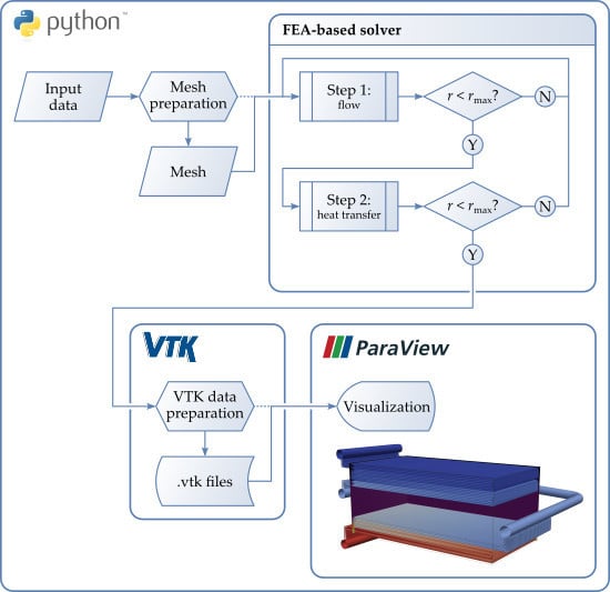
The computer code was developed in Python [38] and utilized NumPy [39] to carry out the necessary matrix computations. The Visualization Toolkit (VTK) [40] and meshio [41] libraries were used to export solution data to Kitware ParaView [42] for visualization. Although no graphical user interface (GUI) is available yet, the authors plan to add it in the future, for example, via the Django web framework [43]. Please note that the code is not publicly available.

Apart from the inclusion of heat transfer, many additional improvements of the code have been made since the publication of the initial article discussing the FEA-based model [26]. The most important one probably is parallelization of the mass flow rate corrector step (please see [26] for details). As the correction algorithm was carried out independently for each mesh edge, a set of asynchronous workers was created using the standard Python multiprocessing library, and the correction tasks were processed in batches on all available CPU cores. This then results in much shorter computational times. Parallelization of the internal matrix computations, however, was not implemented because, given the numbers of elements in the simplified meshes, the matrices were rather small. In other words, the CPU time saved by parallel solution would be wasted on auxiliary operations needed to split the task to multiple cores, thus rendering the net improvement either negligible or even negative.

3. Results

In this section, two test cases are discussed to demonstrate the capabilities of the present version of the developed model. First, a simple cross-flow tube bundle heat exchanger from the literature is evaluated in Section 3.1. Section 3.2 then focuses on a heat recovery hot water boiler in an existing combined heat and power plant, for which stream data have been provided by its operator.

3.1. Simple Cross-Flow Tube Bundle Heat Exchanger from the Literature

The example discussed here was taken from [44] and involves an air-to-water heat exchanger from Figure 7. Its parameters are listed in

Table 2. Parameters of the air-to-water heat exchanger (for the remaining construction data, etc., please see [44]) and the corresponding results obtained using the present model and HTRI Xchanger Suite (“HTRI XS”).

Parameter	Literature [44]	Present Model	HTRI XS
TS 1 inlet conditions	3.0 kg s−1, 25 °C, 500 kPa
TS outlet temperature	37.0 °C	37.5 °C	36.3 °C
TS pressure drop	2.24 kPa	3.01 kPa	1.9 kPa
SS 2 inlet conditions	2.7 kg s−1, 95 °C, 200 kPa
SS outlet temperature	40.0 °C	37.6 °C	42.8 °C
SS pressure drop	1.40 kPa	1.38 kPa	1.2 kPa
heat duty	150.3 kW	156.6 kW	143.0 kW

¹ Tube side (water); ² Shell side (air).

together with the data obtained using the present model and HTRI Xchanger Suite 8.0.1 [45]. The computational time needed by the present model to automatically create the necessary meshes, reach in 46 major iterations the results mentioned below, and export all the solution data into Kitware ParaView for visualization purposes was ca. 15 s on an average desktop computer with the Intel Core i-5 2500K CPU. The ranks of the matrices used in the model were ca. 800 and ca. 1600 in case of fluid flow and heat transfer, respectively.

In order to minimize the number of sources of discrepancies, the necessary heat transfer coefficients were calculated by the present model using the equations mentioned in the literature [44]. The results should, therefore, have been identical, yet they were not. The reason for the difference became clear once one noticed that, in [44], the iterative computation was stopped while the difference between the hot and the cold heat duties was still relatively large. In fact, should one carry out the heat balance for the data from the literature, one would get the actual water heat duty of 150.3 kW (as listed among the results) while for air the duty would be 149.9 kW. There may also be another reason for the discrepancies in the data, namely the fact that, in [44], the computation was done using average temperatures, average fluid physical properties, etc. for the entire tube side and shell side.

Considering the differences between the values provided by the present model and the data yielded by HTRI Xchanger Suite, these most likely stemmed from the software package using much more accurate equations for obtaining the heat transfer coefficients. It, therefore, is entirely possible that with different equations the results obtained using the present model would be much closer to the data from HTRI Xchanger Suite. In any case, this supports the notion that any such tool or model can only be as good as the equations internally utilized by it.

To demonstrate the level of detail of the solution data provided by the developed software, the water and air temperatures were exported (together with the respective geometry, which used only plain tubes to improve clarity) into Kitware ParaView. The resulting combined plot is shown in Figure 8.

3.2. Heat Recovery Hot Water Boiler in an Existing Plant

A heat recovery hot water boiler with nominal thermal power of 53.3 MW in an existing combined heat and power (CHP) plant was selected as the second test case. The boiler contained two counter-flow tube bundles which were mounted in the vertical portion of the flue gas duct (i.e., the tubes are horizontal, see Figure 9). Both bundles consisted of several passes, and each pass was composed of four staggered tube rows with 48 tubes per row. In the bottom bundle, the first pass was unfinned, the second pass used plain round fins, and serrated fins were utilized in the third pass. The top bundle contained solely tubes enhanced with serrated fins. The built-up area of the heated portion of each bundle was ca. 7.6 × 4.0 m. All stream-related data presented in this article were obtained by the operator of the boiler in the course of a guarantee test.

The boiler was driven by flue gas exiting from a gas turbine. Because the temperature field (see the measurement array shown in Figure 9) was almost uniform, the corresponding boundary condition was specified in both the models discussed further as a constant. The outlet temperature of flue gas was estimated by the operator because the respective quantity had not been measured during the guarantee test. All the necessary data are summarized in

Table 3. Data provided by the operator of the heat recovery hot water boiler.

Parameter	Value
tube side fluid	water
tube side inlet conditions	141.7 kg s−1, 48.0 °C, 1,071.7 kPa
tube side outlet temperature	139.3 °C
tube side pressure drop	32.15 kPa
shell side fluid	flue gas
shell side inlet conditions	124.5 kg s−1, 453.9±3.6 °C 1, 101.31 kPa
shell side outlet temperature	ca. 70 °C 2
shell side pressure drop	1.61 kPa
heat duty	53.3 MW

¹ Calculated from time-dependent data obtained using the measurement array shown in Figure 9; ² Estimated (not measured during the guarantee test).

.

The simulation carried out using the developed computer code mentioned in Section 2.3 included both water distribution in the tube side and heat transfer between the flue gas and water. To assess the accuracy of the predicted temperatures, the boiler was also analyzed using an industry-standard tool, namely, HTRI Xchanger Suite. Please note that, with respect to the requests of the manufacturer of the boiler and the operator of the CHP plant, no other data regarding the apparatus can be explicitly specified in this article. For the same reason, neither the HTRI Xchanger Suite case files nor the simplified 3-D CFD model of the flue gas duct discussed in the following sections can be made available.

3.2.1. Simulation in HTRI Xchanger Suite

Compared to a full-scale CFD simulation of the boiler, which would rarely be done in the case of equipment of such size, the actual computational time required by HTRI Xchanger Suite was negligible (units of seconds). Unlike CFD, however, the software generally focuses on the thermal side of the apparatus design, i.e., its primary goal is to provide as accurate stream temperatures as possible while the flows in both the tube and shell sides are assumed to be uniformly distributed (unless the user specifies the distribution explicitly). Moreover, one cannot directly set tube inner and outer surface roughnesses, which may significantly influence the predicted pressure drops.

Results obtained using the discussed software package are listed in

Table 4. Results obtained using HTRI Xchanger Suite and the corresponding errors compared to the data from the operator of the boiler. It is apparent that the temperatures and the tube-side pressure drop were predicted quite accurately, but the shell-side pressure drop was markedly below the measured value.

Parameter	Value	Error
tube side outlet temperature	136.9 °C	−2.4 °C (−1.7%)
tube side pressure drop	32.33 kPa	+0.18 kPa (−0.6%)
shell side outlet temperature	59.3 °C	ca. −10.7 °C (−15%)
shell side pressure drop	0.93 kPa	−0.68 kPa (−42%)
heat duty	53.1 MW	−0.2 MW (−0.4%)

together with the data provided by the operator of the heat recovery hot water boiler. The table also mentions the absolute and relative errors. From these, one can see that the predictions of both the outlet temperatures and the tube-side pressure drop were quite accurate. The predicted shell-side pressure drop, however, was markedly lower than the measured value. It also was a notable disadvantage that no detailed information was given by HTRI Xchanger Suite regarding the actual flow distributions in the bundles and the shell.

3.2.2. Assessment of the Shell-Side Flow Behavior

In order to verify whether the assumption of uniform velocity distribution over the flue gas duct cross-section was appropriate in the FEA-based computation discussed in the next section, a simplified 3-D CFD model of the duct was created in ANSYS Fluent [46]. Parameters of the model are listed in

Table 5. Parameters of the simplified 3-D CFD model of the flue gas duct.

Parameter	Value
solver	pressure-based, transient
pressure–velocity coupling	SIMPLE
transient formulation	2nd order implicit, time step: 0.01 s
active equations	flow, turbulence
turbulence model	Realizable k–ε, Scalable Wall Functions
discretization	2nd order (pressure), 2nd order upwind (other quantities)
inlet/outlet types	mass flow inlet, pressure outlet

. To keep computational demand at a reasonable level, the bundles were replaced by porous zones. Additionally, the entire duct was split into several parts, and hexahedral cells were used whenever possible to further lower the cell count while maintaining acceptable mesh quality. After the necessary mesh adaptation, the final cell count was ca. 3.3 M (see the y⁺ histogram in Figure 10). As for cell equiangle skewness, only 1231 cells (ca. 0.04% of the total number of cells) featured skewness greater than 0.6, of which 1227 fell between 0.6 and 0.7. The obtained contour plot of velocity magnitude just below the bottom bundle is then shown in Figure 11. This indicates that, although the velocity distribution was not entirely uniform (see also the pathlines in Figure 12), the non-uniformity was still at a reasonable level, which should not lead to significant inaccuracy in the calculated overall heat transfer rate.

3.2.3. Present Model

The data yielded by the present, FEA-based model are listed in

Table 6. Results obtained using the present model and the corresponding errors compared to the data from the operator of the boiler. The accuracy was not as good as in the case of HTRI Xchanger Suite, but, in terms of fast, approximate analyses of process and power equipment, it was sufficient.

Parameter	Value	Error
tube side outlet temperature	136.1 °C	−3.2 °C (−2.3%)
tube side pressure drop	30.33 kPa	−1.82 kPa (−5.7%)
shell side outlet temperature	62.9 °C	ca. −7.1 °C (−10%)
shell side pressure drop	1.14 kPa	−0.47 kPa (−29%)
heat duty	52.6 MW	−0.7 MW (−1.3%)

together with the values provided by the operator of the boiler. Here, the accuracy was slightly lower than that of HTRI Xchanger Suite, but it still was acceptable. The computational time needed to automatically create the meshes, reached in 39 major iterations the solution, and export the necessary solution data into Kitware ParaView for visualization purposes was ca. 240 s on the same average desktop computer used in the previous example. The ranks of the matrices were ca. 9000 and ca. 18,500 in case of fluid flow and heat transfer, respectively.

As mentioned before, the present model uses a one-dimensional mesh to represent the shell side. This means that the predicted temperature distribution was, too, only one-dimensional, while flow distribution across the shell-side cannot be predicted at all. In the tube side, on the other hand, the mass flow rate was known for each individual tube, and the predicted temperature distribution was spatially as fine or as coarse as the utilized tube bundle mesh. Figure 13 shows the predicted shell-side temperature distribution along the portion of the flue gas duct enclosing the two bundles, which was obtained using the present model, and the corresponding temperatures provided by the operator of the boiler and yielded by HTRI Xchanger Suite. The temperature curve yielded by the model matches the point values reasonably well with the discrepancies being most likely caused by the usage of different equations for the calculation of the necessary heat transfer coefficients.

Similarly as before, a combined plot of water and flue gas temperatures was generated using Kitware ParaView. This is shown in Figure 14.

The obtained tube mass flow rates were distributed quite uniformly in both bundles. The actual relative standard deviations from uniform flow distribution computed using

$$\delta =\frac{100}{{\dot{m}}_{\mathrm{id}}}\sqrt{\frac{1}{n}{{\displaystyle \sum }}_{i=1}^n{\left({\dot{m}}_i-{\dot{m}}_{\mathrm{id}}\right)}^2},$$

(15)

where ${\dot{m}}_{\mathrm{id}}$ denotes the ideal mass flow rate through one tube of the bundle, n the number of tubes therein, and ${\dot{m}}_i$ the mass flow rate through the ith tube, were 0.3% and 0.4% in case of the top bundle and the bottom bundle, respectively.

4. Discussion

The results yielded by the present model and by HTRI Xchanger Suite for the air-to-water heat exchanger from the literature have shown that even though an apparatus can be decomposed into parts for which correlations or calculation procedures for heat transfer coefficients and pressure losses may exist, successfully applying them may not be straightforward. The main reason is that such procedures require local fluid and material properties, and these generally depend on the temperature and pressure, that is, quantities which the designer is trying to calculate. This is where the present model steps in. The data have also highlighted the facts that the accuracy of any model depends to a large degree on the quality of equations utilized for the calculation of the various coefficients and that further research in this area is, therefore, necessary. Additionally, one can draw the conclusion that using averaged values for the entire tube side and shell side can lead to notable differences. In the case of the outlet temperatures in this air-to-water heat exchanger, it was up to ca. ±7%.

As for the heat recovery hot water boiler, the most important stream parameters are listed in

Table 7. Summary of the main results obtained using the two discussed approaches alongside the data provided by the operator of the boiler.

Parameter	Present Model	HTRI Xchanger Suite	Operator
TS 1 outlet temperature	136.1 °C	136.9 °C	139.3 °C
TS pressure drop	30.33 kPa	32.33 kPa	32.15 kPa
SS 2 outlet temperature	62.9 °C	59.3 °C	ca. 70 °C 3
SS pressure drop	1.14 kPa	0.93 kPa	1.61 kPa
heat duty	52.6 MW	53.1 MW	53.3 MW

¹ Tube side (water); ² Shell side (flue gas); ³ Estimated (not measured during the guarantee test).

. It can be seen that the tube-side outlet temperature and pressure drop were better predicted by HTRI Xchanger Suite, while the accuracy of the shell-side outlet temperature and pressure drop predictions was higher in the case of the present model. Overall, the accuracy of the model was deemed acceptable concerning its intended purpose.

A significant advantage of the model over the industry-standard design package offered by HTRI (or other commonly used heat transfer equipment design packages) lies in the fact that it provides detailed data on the tube-side fluid flow and temperature distributions. This information can be of great value when trying to prevent certain types of operating problems (e.g., excessive thermal loading of the tubes in the bundle and the subsequent mechanical failures). Another advantage is that in the case of cross-flow tube bundles (the primary target application of the present model), HTRI Xchanger Suite assumes that mixing of tube streams occurs after each pass, even if this may not actually be true. Such a simplification may increase convergence, but it also may diminish local effects and, therefore, introduce errors into the data.

5. Conclusions

The point of this research was not to develop a replacement to the universally applicable, commercial heat transfer equipment design packages, such as HTRI Xchanger Suite. On the contrary, the goal was to create a simplified model for heat exchangers representable using sets of interconnected 1-D meshes, which are typically used in high-temperature (i.e., heat recovery) industrial applications and are prone to suffer from operating problems. The model, once finished, should be fast, yet accurate enough, and should provide estimates of not only the flow distribution in the bundle and the tube- and shell-side temperature fields but also the resulting mechanical stress field in the bundle caused by uneven thermal loading. In other words, the aim was to have a supplementary tool which would enable the designer to evaluate in advance, and without any significant effort or time spent, the thermal-hydraulic behavior of the mentioned heat exchangers as well as the likelihood of them suffering mechanical failures under the design operating conditions. In this regard, the FEA-based modelling approach seems to be promising, but a lot of work, as well as a thorough validation, are still needed before it is ready for production use.

The comparison with HTRI was mentioned in this paper solely to present the current capabilities of the model in terms of heat transfer prediction. The discrepancy (or at least a part of it) was very likely caused by the heat transfer coefficients and the hydraulic resistance coefficients being calculated differently. However, the model was designed in such a way that it can easily incorporate any standard method for calculating these coefficients for the simple 1-D mesh elements. More complex flow systems can then be built from these simple elements and the solution strategy remains the same, which ensures scalability of the model.

Considering the fact that shell-side flow velocity fields commonly are not uniform, one of the possible future improvements of the FEA-based model could lie in strictly using a grid of cells in the shell side (in the plane perpendicular to the general direction of flow) instead of only one cell. Another enhancement, which the authors plan to implement, is to make it possible to interface the current computer code with other simulation codes. This would enable the evaluation of flow systems in which some parts are more complex and, therefore, not directly compatible with the simplified mesh elements used by the FEA-based model.

References

1. Wei, H.; Yang, X.; Ge, Z.; Yang, L.; Du, X. Anti-freezing of natural draft dry cooling system of power generation by water re-distribution during winter. Int. J. Heat Mass Transf. 2020, 149, 119194. [Google Scholar] [CrossRef]
2. Chien, N.B.; Linh, N.X.; Jong-Taek, O. Numerical optimization of flow distribution inside inlet header of heat exchanger. Energy Procedia 2019, 158, 5488–5493. [Google Scholar] [CrossRef]
3. Zhou, J.; Ding, M.; Bian, H.; Zhang, Y.; Sun, Z. Characteristics of flow distribution in central-type compact parallel flow heat exchangers with modified inlet and header. Appl. Therm. Eng. 2020, 166, 114636. [Google Scholar] [CrossRef]
4. Łopata, S.; Ocłoń, P.; Stelmach, T. Investigation of flow non-uniformities in the cross-flow heat exchanger with elliptical tubes. E3S Web Conf. 2019, 108, 01009. [Google Scholar] [CrossRef]
5. García-Guendulain, J.M.; Riesco-Ávila, J.M.; Picón-Núñez, M. Reducing thermal imbalances and flow nonuniformity in solar collectors through the selection of free flow area ratio. Energy 2020, 194, 116897. [Google Scholar] [CrossRef]
6. Karvounis, P.; Koubogiannis, D.; Hontzopoulos, E.; Hatziapostolou, A. Numerical and experimental study of flow characteristics in solar collector manifolds. Energies 2019, 12, 1431. [Google Scholar] [CrossRef] [Green Version]
7. Li, M.; Hao, J.; Chen, W.; Li, W. Experimental and theoretical investigations on reverse flow characteristics in vertically inverted U-tube steam generator under transient condition. Prog. Nucl. Energy 2020, 120, 103216. [Google Scholar] [CrossRef]
8. Klenov, O.P.; Noskov, A.S. Influence of input conditions on the flow distribution in trickle bed reactors. Chem. Eng. J. 2020, 382, 122806. [Google Scholar] [CrossRef]
9. He, Y.; Sun, Z.; Shen, B.; Guo, F.; Yang, Y.; Zhan, X.; Li, X. CFD study on the flow distribution of an annular multi-hole nozzle. Can. J. Chem. Eng. 2020, 98, 590–606. [Google Scholar] [CrossRef]
10. Bürkle, F.; Moyon, F.; Feierabend, L.; Wartmann, J.; Heinzel, A.; Czarske, J.; Büttner, L. Investigation and equalisation of the flow distribution in a fuel cell stack. J. Power Sources 2020, 448, 227546. [Google Scholar] [CrossRef]
11. Heck, J.D.; Vaz, W.S.; Koylu, U.O.; Leu, M.C. Decoupling pressure and distribution effects of flow fields on polymer electrolyte fuel cell system performance. Sustain. Energy Technol. Assess. 2019, 36, 100551. [Google Scholar] [CrossRef]
12. Hur, D.-J.; Jeong, S.-H.; Song, S.-I.; Noh, J.-H. Optimization based on product and desirability functions for flow distribution in multi-channel cooling systems of power inverters in electric vehicles. Appl. Sci. 2019, 9, 4844. [Google Scholar] [CrossRef] [Green Version]
13. Li, H.; Ding, X.; Jing, D.; Xiong, M.; Meng, F. Experimental and numerical investigation of liquid-cooled heat sinks designed by topology optimization. Int. J. Therm. Sci. 2019, 146, 106065. [Google Scholar] [CrossRef]
14. Zhu, J.; Zhang, W.; Li, Y.; Ji, P.; Wang, W. Experimental study of flow distribution in plate-fin heat exchanger and its influence on natural gas liquefaction performance. Appl. Therm. Eng. 2019, 155, 398–417. [Google Scholar] [CrossRef]
15. Tang, H.; Zhang, T.; Liu, X.-H. Experimental study on refrigerant maldistribution in a fin-and-tube evaporator for a direct expansion air-conditioning system. Energy Build. 2020, 208, 109638. [Google Scholar] [CrossRef]
16. Quintanar, N.R.; Nguyen, T.; Vaghetto, R.; Hassan, Y.A. Natural circulation flow distribution within a multi-branch manifold. Int. J. Heat Mass Transf. 2019, 135, 1–15. [Google Scholar] [CrossRef]
17. Yih, J.; Wang, H. Experimental characterization of thermal-hydraulic performance of a microchannel heat exchanger for waste heat recovery. Energy Convers. Manag. 2020, 204, 112309. [Google Scholar] [CrossRef]
18. Lugarini, A.; Franco, A.T.; Errera, M.R. Flow distribution uniformity in a comb-like microchannel network. Microfluid. Nanofluid. 2019, 23, 44. [Google Scholar] [CrossRef]
19. Ishiyama, E.M.; Pugh, S.J. Effect of flow distribution in parallel heat exchanger networks: Use of thermo-hydraulic channeling model in refinery operation. Heat Transf. Eng. 2020, 41, 189–198. [Google Scholar] [CrossRef]
20. Novitsky, N.N.; Alekseev, A.V.; Grebneva, O.A.; Lutsenko, A.V.; Tokarev, V.V.; Shalaginova, Z.I. Multilevel modeling and optimization of large-scale pipeline systems operation. Energy 2019, 184, 151–164. [Google Scholar] [CrossRef]
21. Korelstein, L. Hydraulic networks with pressure-dependent closure relations, under restrictions on the value of nodal pressures. Maxwell matrix properties and monotonicity of flow distribution problem solution. E3S Web Conf. 2019, 102, 01005. [Google Scholar] [CrossRef]
22. Cassiolato, G.; Carvalho, E.P.; Caballero, J.A.; Ravagnani, M.A. Optimization of water distribution networks using a deterministic approach. Eng. Optim. 2020. [Google Scholar] [CrossRef]
23. Sun, L.; Yan, H.; Xin, K.; Tao, T. Contamination source identification in water distribution networks using convolutional neural network. Environ. Sci. Pollut. Res. 2019, 26, 36786–36797. [Google Scholar] [CrossRef] [PubMed]
24. Fang, Q.-S.; Zhang, J.-X.; Xie, C.-L.; Yang, Y.-L. Detection of multiple leakage points in water distribution networks based on convolutional neural networks. Water Supply 2019, 19, 2231–2239. [Google Scholar] [CrossRef]
25. Jeong, G.; Kang, D. Hydraulic uniformity index for water distribution networks. J. Water Resour. Plan. Manag. 2020, 146, 04019078. [Google Scholar] [CrossRef]
26. Létal, T.; Turek, V.; Fialová, D. Nonlinear finite element analysis-based flow distribution model for engineering practice. Chem. Eng. Trans. 2019, 76, 157–162. [Google Scholar] [CrossRef]
27. Fialová, D. Flow Distribution in Equipment with Dense Tube Bundles. Master’s Thesis, Brno University of Technology, Brno, Czech Republic, 2017. (In Czech). [Google Scholar]
28. Gnielinski, V. Heat Transfer in cross-flow around single rows of tubes and through tube bundles. In VDI Heat Atlas, 2nd ed.; Part, G., Stephan, P., Kabelac, S., Kind, M., Martin, H., Mewes, D., Schaber, K., Eds.; Springer: Berlin, Germany, 2010; pp. 725–730. [Google Scholar] [CrossRef]
29. Webb, R.L.; Kim, N.-H. Externally finned tubes. In Principles of Enhanced Heat Transfer, 2nd ed.; Taylor & Francis Group: New York, NY, USA, 2005. [Google Scholar]
30. Lindqvist, K.; Næss, E. A validated CFD model of plain and serrated fin-tube bundles. Appl. Therm. Eng. 2018, 143, 72–79. [Google Scholar] [CrossRef]
31. Lindqvist, K.; Wilson, Z.T.; Næss, E.; Sahinidis, N.V. A machine learning approach to correlation development applied to fin-tube bundle heat exchangers. Energies 2018, 11, 3450. [Google Scholar] [CrossRef] [Green Version]
32. Hofmann, R.; Heimo, W. Experimental and numerical investigation of the gas side heat transfer and pressure drop of finned tubes—Part I: Experimental analysis. J. Therm. Sci. Eng. Appl. 2012, 4, 041007. [Google Scholar] [CrossRef]
33. Hofmann, R.; Heimo, W. Experimental and numerical investigation of the gas side heat transfer and pressure drop of finned tubes—Part II: Numerical analysis. J. Therm. Sci. Eng. Appl. 2012, 4, 041008. [Google Scholar] [CrossRef]
34. Python Implementation of the IAPWS Standard. Available online: https://github.com/jjgomera/iapws (accessed on 21 January 2020).
35. Bell, I.H.; Wronski, J.; Quoilin, S.; Lemort, V. Pure and pseudo-pure fluid thermophysical property evaluation and the open-source thermophysical property library CoolProp. Ind. Eng. Chem. Res. 2014, 53, 2498–2508. [Google Scholar] [CrossRef] [PubMed] [Green Version]
36. European Committee for Standardization. EN 12952-2:2011. Water-Tube Boilers and Auxiliary Installations—Part 2: Materials for Pressure Parts of Boilers and Accessories; European Committee for Standardization: Brussels, Belgium, 2011. [Google Scholar]
37. Ganapathy, V. Finned tubes. In Waste Heat Boiler Deskbook; The Fairmont Press, Inc.: Lilburn, GA, USA, 1991; Appendix A; pp. 275–306. [Google Scholar]
38. Python Language Reference, Version 3.8.1. Available online: https://www.python.org (accessed on 21 January 2020).
39. Oliphant, T.E. A Guide to NumPy; Trelgol Publishing: Spanish Fork, UT, USA, 2006. [Google Scholar]
40. Schroeder, W.; Martin, K.; Lorensen, B. The Visualization Toolkit, 4th ed.; Kitware, Inc.: Clifton Park, NY, USA, 2006. [Google Scholar]
41. I/O for Mesh Files. Available online: https://github.com/nschloe/meshio (accessed on 21 January 2020).
42. Ayachit, U. The ParaView Guide: A Parallel Visualization Application; Kitware, Inc.: Clifton Park, NY, USA, 2015. [Google Scholar]
43. Django, Version 3.0.2. Available online: https://djangoproject.com (accessed on 21 January 2020).
44. Pismennyi, E.; Polupan, G.; Carvajal-Mariscal, I.; Sanchez-Silva, F.; Pioro, I. Examples of calculations. In Handbook for Transversely Finned Tube Heat Exchanger Design; Academic Press: Cambridge, MA, USA, 2016; Chapter 7; pp. 83–106. [Google Scholar] [CrossRef]
45. Heat Transfer Research, Inc. HTRI Xchanger Suite User’s Guide, Version 8.0.1; Heat Transfer Research, Inc.: Navasota, TX, USA, 2019. [Google Scholar]
46. ANSYS, Inc. ANSYS Fluent User’s Guide, Version 2019 R3; ANSYS, Inc.: Canonsburgh, PA, USA, 2019. [Google Scholar]
Figure 1. Schematic of the flow distribution system from Table 1.
Energies 13 01664 g001
Figure 2. (a) Tube mass flow rates obtained for the flow system from Table 1 using the model based on Finite Element Analysis (FEA) discussed in [26] and a transient Computational Fluid Dynamics (CFD) simulation. Average tube Reynolds number was ca. 1500. (b) The corresponding relative tube mass flow rate errors (FEA vs. CFD simulation). Tube numbers correspond to Figure 1. For the details regarding the CFD model, the reader is kindly referred to [27].
Energies 13 01664 g002
Figure 3. Comparison of the fluid flow mesh (left) and the temperature mesh (right). The fluid flow mesh consists of 8 edges with 8 nodes total, and there are 8 unknown pressures (in the green nodes, some of which are shared between edges); in the temperature mesh, there are 2 × 8 = 16 nodes and, therefore, 16 unknown temperatures.
Energies 13 01664 g003
Figure 4. Internal flows in a system vs. flow mixing; there are 4 locations (the T-joints) for which the flow mixing/splitting equations must be present in the final linear system.
Energies 13 01664 g004
Figure 5. A pair of adjacent control volumes representing a portion of the tube side and the enclosing portion of the shell side.
Energies 13 01664 g005
Figure 6. Non-zero values in the sparse temperature field matrix used in the second step of the FEA solver. Please note that, for the sake of clarity, only a small matrix with the rank slightly below 800 is shown here, which originates from a flow distribution system with two bundles consisting of just four tubes each.
Energies 13 01664 g006
Figure 7. The evaluated air-to-water heat exchanger (please note that the tubes are shown as unfinned for clarity even though the exchanger used rolled helical fins in the heated portion of the bundle). The dimensions of the air duct were 0.56 × 0.5 × 1.0 m (width × height × length).
Energies 13 01664 g007
Figure 8. Visualization generated in Kitware ParaView of the bundle in the air duct (some faces are culled). These were colored by the tube-side (water) and the shell-side (air) temperatures obtained using the FEA-based model.
Energies 13 01664 g008
Figure 9. Schematic of the investigated boiler. Top bundle collector was connected to the bottom bundle distributor via an external duct as indicated using the dashed lines. The temperature field measurement array, consisting of 12 (4 × 3) sensors, was only installed in the duct during the guarantee test.
Energies 13 01664 g009
Figure 10. Histogram of y+ values of wall-adjacent cells in the model from Table 5. There were 275 cells with y+ ≤ 30 (all of these but 12 were between 25 and 30, ca. 0.04% of the total number of wall-adjacent cells) and no cells with y+ > 300.
Energies 13 01664 g010
Figure 11. Contour plot of velocity magnitude just below the bottom bundle, which was obtained using the CFD model from Table 5. The velocity distribution was not uniform (due to the flue gas duct being bent) and fluctuated in time.
Energies 13 01664 g011
Figure 12. Pathlines in the flue gas duct, which were colored by velocity magnitude. One can see that the flow behind the bend is pushed to one side as indicated in Figure 11 and that there are relatively large recirculation zones present.
Energies 13 01664 g012
Figure 13. Comparison of the temperature distribution in the portion of the flue gas duct enclosing the two bundles, which was obtained using the present model, and the corresponding temperatures provided by the operator of the boiler and yielded by HTRI Xchanger Suite (“HTRI XS”). Vertical distance along the channel corresponds to the distance from the point denoted “y = 0 m” in Figure 9.
Energies 13 01664 g013
Figure 14. Visualization generated in Kitware ParaView of the bundles and the surrounding portion of the flue gas duct (front faces are culled). These were colored by the tube-side (water) and the shell-side (flue gas) temperatures obtained using the FEA-based model.
Energies 13 01664 g014