Article

Second-Order Approximation of the Seismic Reflection Coefficient in Thin Interbeds

1
Key Laboratory of Earth and Planetary Physics, Institute of Geology and Geophysics, Chinese Academy of Sciences, Beijing 100029, China
2
University of Chinese Academy of Sciences, Beijing 100049, China
3
School of Geophysics and Information Technology, China University of Geosciences, Beijing 100083, China
*
Author to whom correspondence should be addressed.
Energies 2020, 13(6), 1465; https://doi.org/10.3390/en13061465
Submission received: 10 February 2020 / Revised: 14 March 2020 / Accepted: 19 March 2020 / Published: 20 March 2020
(This article belongs to the Section H: Geo-Energy)

Abstract

:
As most of the lithostratigraphic reservoirs in China are thin interbeds, the study of seismic responses in thin interbeds is an integral part of lithologic reservoir exploration. However, at present, the research on seismic reflection coefficients of thin interbeds in exploration seismology is still weak, which leads to the lack of theoretical basis for the subsequent interpretation of amplitude variation with offset (AVO) related to thin interbed. To solve this problem, in this paper, we proposed second-order approximate equations of the seismic reflection coefficients in thin-bed and thin-interbed layers. Under the assumption of a small impedance contrast in layered media, we made a second-order approximation with a more evident physical meaning to the reflection coefficient calculation method proposed by Kennett. Then, based on the test of the single thin-layer theoretical model, it was confirmed that the second-order approximation equation of the PP-wave (reflected compressional wave) is accurate at incident angles less than 30°, and that of the PS-wave (converted shear wave) is accurate at wider incident angles. Finally, based on the single-thin-bed equations, the approximate equations of seismic reflection coefficients in thin interbeds were established, the validity of which was verified by the theoretical model. Our equations will be applicable to the calculation of PP- and PS-wave reflection coefficients in thin interbeds where internal multiples are difficult to suppress and transmission loss is hard to accurately compensate. This lays a theoretical foundation for improving the seismic prediction accuracy of lithologic reservoirs.

1. Introduction

The technology of amplitude versus offset (AVO) or amplitude versus incident angle (AVA) has been used to predict rock properties and fluid in the subsurface reservoirs for decades [1,2,3,4]. Conventional AVO analysis is based on Zoeppritz equations or their approximations; however, these equations are not suitable for thin-bed problems due to the mixing of the reflected waves, converted waves, and internal multiples, which are hard to separate [5,6,7].
The problem of thin-bed layers has been studied for decades. Typically, a single layer with a thickness of less than a quarter of a wavelength is defined as a thin layer in seismology [8,9]. Brekhovskikh [10,11] gave the displacement potential reflections and transmissions of plane waves propagating in layered elastic media. Kennett [12] proposed the recursive algorithm for the calculation of total reflection and transmission coefficients for a stack of layers, in which the unconditional stability for all frequencies and slownesses was improved. The recursive algorithm solved the overflow problems in the calculation of exponential functions for high frequencies and slownesses [13,14]. Liu and Schmitt [15] proposed an exact analytical solution in the acoustic wave domain and simulated the reflection amplitude and AVO responses of a single thin bed for arbitrary incident angles. Pan and Innanen [6] simplified the elastic multi-layered medium equation based on Breshkovskikh’s equations to analyze the relationship between the AVO effect and frequency in thin elastic media. Yang et al. [16] derived thin-bed reflection and transmission coefficients defined in terms of displacements and approximated them to be in a quasi-Zoeppritz matrix form under the assumption of a very thin thickness for the thin bed. Yang et al. [17] proposed a low-order series approximation of thin bed for PP-wave, and estimated the P-wave (compressional wave) impedance ratios and thickness. Lu et al. [18] equated the set of thin interlayers with vertical transverse isotropic stratigraphy and used the reflection coefficients of anisotropic media for AVO inversion study.
In general, the existing approximate equations of thin-bed reflection coefficients are based on the assumption of small incident angle and weak impedance contrast. Additionally, these equations are complicated and their physical meaning is not clear, so they do not easily provide theoretical support for the subsequent AVO interpretation of single thin beds or thin interbeds. In this paper, we performed a numerical simulation analysis on the single thin-bed model based on the Kennett equation and found that the high-order multiples contribute less to the overall reflection coefficient of the single thin bed. Thus, we deduced the second-order approximate equation with a more evident physical meaning of the reflection coefficient in a single thin-bed, which is suitable for both PP- and PS-waves. Further, we used a recursive algorithm [12] to extend the second-order approximation equation of the thin-bed reflection coefficient to the thin-interbed model and verified its accuracy by numerical simulation analysis.

2. Exact Reflection Coefficient Equation in Stratified Media

Our single thin-bed reflection coefficient equation is deduced based on the exact reflection coefficient equation in stratified media proposed by Kennett [13,14]. For the stratified strata, as shown in Figure 1, A and C are the top and bottom interfaces, respectively, and B is an interface inside the model. The down-going wave (denoted by subscript ‘D’) propagates in area AC (the area between interfaces A and C), generating reflected waves, converted waves, and internal multiples. These wavefields are mixed together, and the up-going waves are denoted by subscript ‘U’. Kennett [13,14] derived the following equation using the recursive algorithm to calculate the overall reflection and transmission coefficient matrices of region AC:
R D AC = r D A + t U A R ^ D BC [ I r U A R ^ D BC ] 1 t D A ,
where r D A and t D A are the single-interface reflection coefficient and transmission coefficient matrices at interface A, respectively:
r D A = [ r PP r PS r SP r SS ] D A ,
t D A = [ t PP t PS t SP t SS ] D A ,
where the superscripts ‘PP’, ‘PS’, ‘SS’, and ‘SP’ represent the four wave modes (P-wave reflected/transmitted to P-wave, P-wave reflected/transmitted to shear wave, shear wave reflected/transmitted to shear wave, shear wave reflected/transmitted to P-wave,) of single interface reflections or transmissions, which can be calculated by Zoeppritz equations [19]. R ^ D BC is obtained from the total reflection matrix R D BC of region BC by phase shift to the bottom of interface A:
R ^ D BC = E R D BC E ,
where E is the phase income for downward propagation through the layer. Furthermore, the following exists:
E = [ e i ω q α h e i ω q β h ] ,
where ω is the angular frequency; h indicates the thickness of region AB; qα and qβ are the vertical slownesses for P- and S-waves (shear wave):
{ q α = 1 α 2 p 2 , q β = 1 β 2 p 2 ,
where α and β are the P- and S-wave velocities, respectively, and p is the horizontal slowness.

3. Second-Order Approximate Reflection of Single Thin-Bed Media

3.1. Assumption of Small to Medium Impedance Contrast

We extracted a single thin bed model from the layered medium model shown in Figure 1. As shown in Figure 2, Layers 1 and 3 are the adjacent overlying and underlying strata of the single thin bed Layer 2, respectively. According to Equation (1), the total reflection matrix at top interface 1 can be written as
R D ( 1 ) = r D ( 1 ) + t U ( 1 ) R ^ D ( 2 ) [ I r U ( 1 ) R ^ D ( 2 ) ] 1 t D ( 1 ) ,
where R ^ D ( 2 ) is the phase-shifted reflection matrix relative to interface 2.
R ^ D ( 2 ) = E ( 2 ) r D ( 2 ) E ( 2 ) ,
where E(2) is the phase income for downward propagation through the thin layer with the thickness h(2),
E ( 2 ) = [ e i ω q α ( 2 ) h ( 2 ) e i ω q β ( 2 ) h ( 2 ) ] ,
the function of which is to move the reflection coefficient matrix r D ( 2 ) to the bottom of interface 1.
Using Taylor’s expansion approach, Equation 7 can be expanded as
R D ( 1 ) = r D ( 1 ) + t U ( 1 ) R ^ D ( 2 ) [ I + n = 1 ( r U ( 1 ) R ^ D ( 2 ) ) n ] t D ( 1 ) ,
where the total reflection matrix R D ( 1 ) is in 2 × 2 form of
R D ( 1 ) = [ R PP R PS R SP R SS ] D ( 1 ) .
Since the current multi-component seismic exploration mainly uses reflected PP- and PS-waves, in this paper, we will only study the reflection coefficients of the reflected PP- and PS-waves. According to the different propagation paths, the PP- and PS-waves relating to R D ( 1 ) can be divided into several modes, as shown in Figure 3 and Figure 4, respectively. The PP-waves in Figure 3 are divided into the following modes based on the wave types in the propagation path: a. PP mode, b. PPPP mode, c. PSPP mode, d. PPSP mode, e. PSSP mode, and f. internal multiples. Here, we take PPPPPP and PPPPPPPP modes as examples. Similarly, according to the wave types in the propagation path, the PS-waves in Figure 4 can be divided into the following modes: a. PS mode, b. PPPS mode, c. PSPS mode, d. PPSS mode, e. PSSS mode, and f. internal multiples. Here, we take PSSSSS and PSSSSSSS modes as examples.
We grade the energy of the internal multiples and retain the multiples that contribute most to the single thin-bed reflection.
Let the absolute amplitude of the incident wave be A0, and the absolute amplitudes of the first-order multiples and second-order multiples in the single thin layer ( Layer 2 ) be A1 and A2, respectively. According to the definition of reflection and transmission coefficients [20], the relationships between A1, A2, and A0 are as follows:
A 1 = A 0 t D ( 1 ) t U ( 1 ) r D ( 2 ) ( r U ( 1 ) r D ( 2 ) ) ,
A 2 = A 0 t D ( 1 ) t U ( 1 ) r D ( 2 ) ( r U ( 1 ) r D ( 2 ) ) 2 .
Similarly, the absolute amplitude An of the nth-order multiples is
A n = A 0 t D ( 1 ) t U ( 1 ) r D ( 2 ) δ n .
where
δ = r U ( 1 ) r D ( 2 ) .
If n = 0, Equation (14) represents the absolute amplitude of the primary reflected wave.
Because the seismic wave energy E is proportional to the square of amplitude and to the primary wave energy EP, we obtain
E P ( A 0 t D ( 1 ) t U ( 1 ) r D ( 2 ) ) 2 .
Thus, for the energy of all internal multiples EM, we obtain
E M ( A 1 2 + A 2 2 + + A n 2 + ) .
Because the range of the reflection coefficients r U ( 1 ) and r D ( 2 ) is (−1, 1), δ < 1. If n approaches infinity, Equation (17) is simplified to
E M ( A 0 t D ( 1 ) t U ( 1 ) r D ( 2 ) ) 2 δ 2 1 δ 2 .
Then, the ratio between the energy of all internal multiples EM and the energy of the primary wave EP is
E M / E P = ( A 0 t D ( 1 ) t U ( 1 ) r D ( 2 ) ) 2 δ 2 1 δ 2 ( A 0 t D ( 1 ) t U ( 1 ) r D ( 2 ) ) 2 = δ 2 1 δ 2 .
The ratio between the energy of first-order multiples EM1 and the energy of all multiples EM is
E M 1 / E M = ( A 0 t D ( 1 ) t U ( 1 ) r D ( 2 ) ) 2 δ 2 ( A 0 t D ( 1 ) t U ( 1 ) r D ( 2 ) ) 2 δ 2 1 δ 2 = 1 δ 2 .
The ratio of the sum energy of the first-order and second-order multiples to the energy of all multiples EM is
E M 2 / E M = ( A 0 t D ( 1 ) t U ( 1 ) r D ( 2 ) ) 2 ( δ 2 + δ 4 ) ( A 0 t D ( 1 ) t U ( 1 ) r D ( 2 ) ) 2 δ 2 1 δ 2 = 1 δ 4 .
Furthermore, the ratio of the sum energy of the first-order, second-order, and third-order multiples to the energy of all multiples EM is
E M 3 / E M = ( A 0 t D ( 1 ) t U ( 1 ) r D ( 2 ) ) 2 ( δ 2 + δ 4 + δ 6 ) ( A 0 t D ( 1 ) t U ( 1 ) r D ( 2 ) ) 2 δ 2 1 δ 2 = 1 δ 6 .
In the derivation of Equations (12)–(22), wave types are not distinguished, so they are applicable to both PP- and PS-waves. Let the reflection coefficient be in the range of (−1, 1); the calculated energy ratios are shown in Figure 5, from which we can conclude the following.
(1) The smaller the absolute value of the reflection coefficient, the smaller the ratio of EM/EP. Figure 5a shows that, as the reflection coefficient decreases, EM/EP also decreases. When the absolute value of the reflection coefficient is less than 0.3, the ratio of EM/EP will be less than 0.1, and the energy ratio corresponds to the blue color in Figure 5a.
(2) The sum of the first- and second-order multiple energies occupies the major part of the internal multiples energy. Figure 5b shows that when the absolute value of the reflection coefficient is less than about 0.3, the energy of the first-order multiples occupies more than 95% of the multiple energy. Besides, it can be seen from Figure 5c that when the absolute value of the reflection coefficient is less than about 0.6, the sum energy of the first- and second-order multiples occupy more than 95% of the multiple energy. In addition, Figure 5d shows that when the absolute values of the reflection coefficients are less than about 0.75, the sum of the energy of the first-, second-, and third-order multiples occupies more than 95% of the multiple energy. In actual seismic data, the absolute values of the reflection coefficients of most strata are less than 0.6. Therefore, for most single thin layers, the contribution of multiple waves in the overall reflection coefficient only needs to take the first- and second-order multiples into account.
According to the energy ratio analysis, if the wave impedance contrast is very small—that is, the reflection coefficient is also extremely small—the energy of internal multiples will be very weak. In this case, internal multiples may not be considered, and then Equation (10) can be approximated as
R D ( 1 ) = r D ( 1 ) + t U ( 1 ) R ^ D ( 2 ) t D ( 1 ) .
Under the condition of moderate impedance contrast (i.e., the absolute value of reflection coefficient is less than 0.6), according to the energy ratio analysis, let n = 2 in Equation (10), and the second-order approximation equation of the total reflection coefficient of the single thin-bed is
R D ( 1 ) = r D ( 1 ) + t U ( 1 ) R ^ D ( 2 ) [ I + r U ( 1 ) R ^ D ( 2 ) + ( r U ( 1 ) R ^ D ( 2 ) ) 2 ] t D ( 1 ) ,
the expansion of which is
R D ( 1 ) = r D ( 1 ) + t U ( 1 ) R ^ D ( 2 ) t D ( 1 ) + t U ( 1 ) R ^ D ( 2 ) r U ( 1 ) R ^ D ( 2 ) t D ( 1 ) + t U ( 1 ) R ^ D ( 2 ) r U ( 1 ) R ^ D ( 2 ) r U ( 1 ) R ^ D ( 2 ) t D ( 1 ) .
As shown in Figure 6, in Equation (25), each item has a clear physical meaning. The details are as follows:
(1)
r D ( 1 ) : the reflection coefficient at the top interface (Interface 1) of the thin bed.
(2)
t U ( 1 ) R ^ D ( 2 ) t D ( 1 ) : the primary reflection coefficient at the bottom interface (Interface 2) of the thin bed, in which the down-going and up-going wave transmission losses ( t U ( 1 ) and t D ( 1 ) ) at Interface 1 are considered;
(3)
t U ( 1 ) R ^ D ( 2 ) r U ( 1 ) R ^ D ( 2 ) t D ( 1 ) : the first-order multiple reflection coefficient of the thin-bed. An additional interaction in the thin-bed is introduced based on the primary reflection.
(4)
t U ( 1 ) R ^ D ( 2 ) r U ( 1 ) R ^ D ( 2 ) r U ( 1 ) R ^ D ( 2 ) t D ( 1 ) : the second-order multiple reflection coefficient of the thin-bed. An additional interaction in the thin-bed is added based on the first-order multiple reflections.
It should be noted that the reflection coefficient calculated by Equation (24) is in the slowness-frequency domain, and can be written as
R D ( 1 ) ( p , ω ) = r D ( 1 ) ( p ) + t U ( 1 ) ( p ) R ^ D ( 2 ) ( p , ω ) [ I + r U ( 1 ) ( p ) R ^ D ( 2 ) ( p , ω ) + ( r U ( 1 ) ( p ) R ^ D ( 2 ) ( p , ω ) ) 2 ] t D ( 1 ) ( p ) .
However, the reflection coefficient used in seismic inversion is mainly in the angle–time domain, and thus a domain conversion is necessary. The entire domain transformation process can be divided into the following two steps.
(1)
Slowness to incident angle
According to Snell’s law, there is
p = sin θ α ,
where θ is the incident angle. Given the incident angle and the P-wave velocity of the overlying formation of the thin layer, the corresponding horizontal slowness can be calculated according to Equation (27), and R D ( 1 ) ( ω , θ ) is further obtained according to Equation (26).
(2)
Frequency domain to time domain
Using an inverse Fourier transform, we can get the reflection coefficient in the intercept time and angle (τ-θ) domain [14,21]:
R D ( 1 ) ( τ , θ ) = 1 2 π R D ( 1 ) ( ω , θ ) e i ω t d ω .
Then, the AVA synthetic seismogram can be obtained by the convolution of the reflection coefficients and wavelets:
Φ ( τ , θ ) = W R D ( 1 ) ( τ , θ ) ,
where W denotes the wavelets.

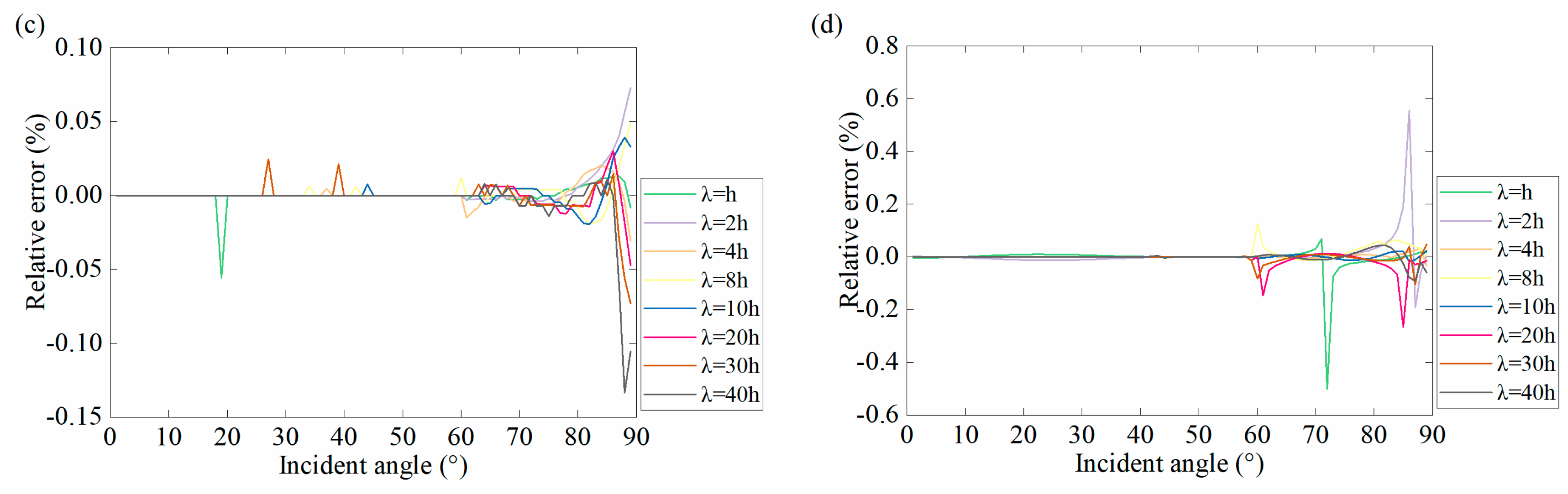
3.2. Accuracy Analysis of Second-Order Approximation

We used a theoretical model to test the accuracy of our second-order approximate equation (Equation (24)) of the single thin-bed reflection coefficient. In the model, the elastic parameters of the first and third layers are fixed and those in the middle layer change with varying impedance contrast. The parameters of the first and third layers are set as α1 = 3.094 km/s, β1 = 1.515 km/s, ρ1 = 2.4 g/cm3, h1 = 150 m. The thickness of the thin bed is 8 m, and its elastic parameters are shown in Table 1 with different P-wave impedance differences between the thin-bed layer and the top layer. Besides, the S-wave velocities and densities of the thin-bed layer are converted from the P-wave velocity according to Castagna equation [22] and Gardner equation [23], respectively. In the numerical simulation, the Ricker wavelets with a dominant frequency of 40 Hz and 30 Hz are used for PP- and PS-waves, respectively [24].
Taking ΔI = −1.5 as an example, Figure 7 and Figure 8 display the angle gathers of PP- and PS-waves, respectively. It can be seen from Figure 7e and Figure 8e that the difference between the angle gather including all the reverberations and the second-order approximation is very small. Besides, Figure 7d and Figure 8d show that the second-order approximate angle gather contains multiples, which are aliased together with the primary waves. It is difficult for the existing technology to eliminate these internal multiples without affecting the energy of primary reflections.
To further quantify the accuracy of the second-order approximation equation, we extract the amplitude along with the top interface of the thin bed, where the amplitude of the second-order approximation is A2, and the amplitude of the data containing all reverberations is Aall. We define the amplitude change ratio Ara as
A ra = A all A 2 A all .
Figure 9 shows the change of Ara with the incident angles of PP- and PS-wave corresponding to the thin-bed model shown in Table 1, from which we can obtain the following rules:
(1)
With the increase of impedance contrasts, Ara also tends to increase.
(2)
If the incident angle exceeds 30°, the error will rapidly increase when using the second-order approximation equation to calculate the PP-wave reflection coefficient. For the PP-wave, initially, Ara is small and increases very slowly with the increasing angle, but after the angle exceeds 30°, Ara increases rapidly.
(3)
The Ara of the PS-wave decreases as the incident angle increases, which shows that the second-order approximation equation is suitable for calculating PS reflections at large angles. However, if the PP- and PS-wave are jointly used for seismic inversion, the applicable angle range of the second-order approximate equation needs to take the intersection of PP- and PS-waves.
In order to test the influence of frequency on the second-order approximate equation, we used waves with different wavelengths (frequencies) to test the single thin-bed model. As shown in Figure 10 and Figure 11, taking ΔI = –1.5 as an example, we calculated the modulus and phase angles of the second-order approximate reflection coefficients of PP- and PS-waves in the frequency domain based on Equations 26 and 27, and compared them with the exact reflection coefficients calculated by the Kennett equation (Equation 7). The wavelengths of the incident waves are set as λ = h, λ = 2h, λ = 4h, λ = 8h, λ = 10h, λ = 20h, λ = 30h, λ = 40h. For the PP-wave, the corresponding frequencies are 333.01 Hz, 166.50 Hz, 83.25 Hz, 41.63 Hz, 33.30 Hz, 16.65 Hz, 11.10 Hz, and 8.33 Hz respectively; for the PS-wave, the corresponding frequencies are 216.78 Hz, 108.39 Hz, 54.19 Hz, 27.10 Hz, 21.68 Hz, 10.84 Hz, 7.23 Hz, and 5.42 Hz, respectively.
Due to the low impedance contrast of the model, the results calculated by the second-order approximate equation and the Kennett equation are very close. The relative percentage errors are shown in Figure 10c,d and Figure 11c,d. The critical angle of the model is about 59.4°. It can be seen that the error is relatively small when the incident angle is within the critical angle. Especially when the thickness is less than half a wavelength, the relative error is almost zero. If the angle of incidence is greater than the critical angle, the error of the second-order approximation equation is relatively large.

4. Second-Order Approximate Reflection of Thin-Interbed Media

4.1. Assumption of Small to Medium Impedance Contrast

Since thin-interbed layers are widespread in the Earth, such as interbeds formed by thin sand and thin mud, it is necessary to expand the approximate equation from the thin bed to thin interbed signal. If several thin layers with small impedance contrasts are superposed together, a set of thin interbeds can be formed. We chose a recursive algorithm [12,13,14] to generate the response of a thin-interbed medium recursively by adding one layer at a time (Figure 12). Since there is no reflection under the bottom interface, the total reflection coefficient of the bottom R D ( n + 1 ) is the same as the reflection coefficient of the single interface r D ( n + 1 ) :
R D ( n + 1 ) = r D ( n + 1 ) = [ r PP r PS r SP r SS ] D ( n + 1 ) .
According to Equation (24), the second-order approximate total reflection coefficient at the top of the nth layer is
R D ( n ) = r D ( n ) + t U ( n ) R ^ D ( n + 1 ) [ I + r U ( n ) R ^ D ( n + 1 ) + ( r U ( n ) R ^ D ( n + 1 ) ) 2 ] t D ( n ) ,
where R ^ D ( n + 1 ) = E ( n ) R D ( n + 1 ) E ( n ) .
The second-order approximate total reflection coefficient at any interface K in the thin interbed can be derived by the recursive algorithm:
R D ( k ) = r D ( k ) + t U ( k ) R ^ D ( k + 1 ) [ I + r U ( k ) R ^ D ( k + 1 ) + ( r U ( k ) R ^ D ( k + 1 ) ) 2 ] t D ( k ) , k [ 1 , n ] ,

4.2. Accuracy Analysis of Second-Order Approximation

Compared with the single thin-bed model, the thin-interbed model will produce more complex internal multiples, which cannot be discriminated by the reflection coefficient curve. Therefore, we will directly use the angle gather to analyze the accuracy of the second-order approximate equation of the thin-interbed model. The thickness of a single thin bed in the thin-interbed model is set as 6 m, and the elastic parameters of the thin-interbed model are shown in Table 2. In the numerical simulation, we used the Ricker wavelet with dominant frequencies of 40 Hz and 30 Hz for PP- and PS-waves, respectively. The angle gathers of the PP- and PS-waves of the thin-interbed model are shown in Figure 13 and Figure 14. In order to avoid wide-angle reflection, the incident angle range is set to 0°–65°. Figure 13 and Figure 14 reveal that:
(1)
The simulated angle gather of the second-order approximate equation is very similar to the angle gather including all reverberations (Figure 13e and Figure 14e).
(2)
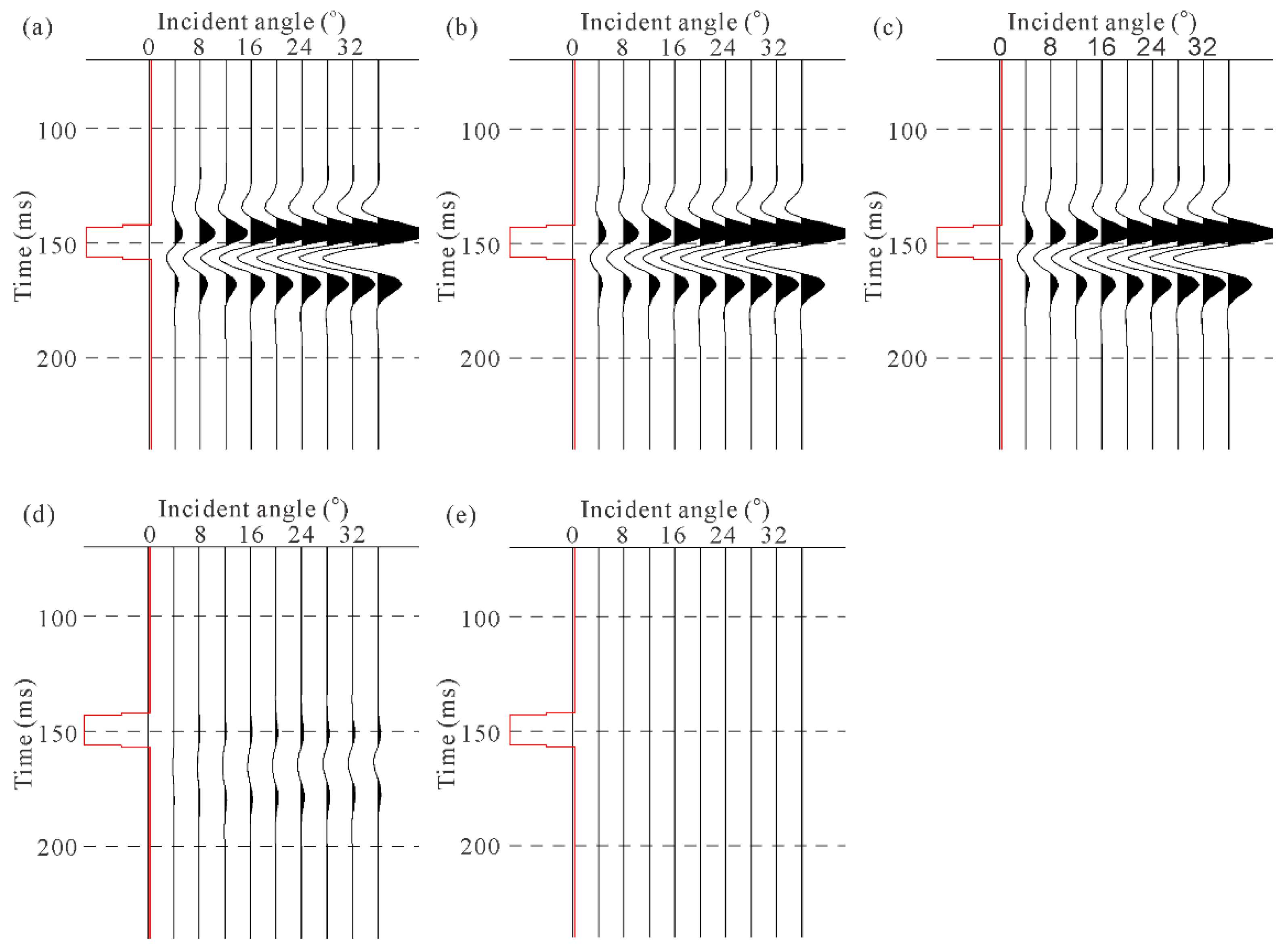
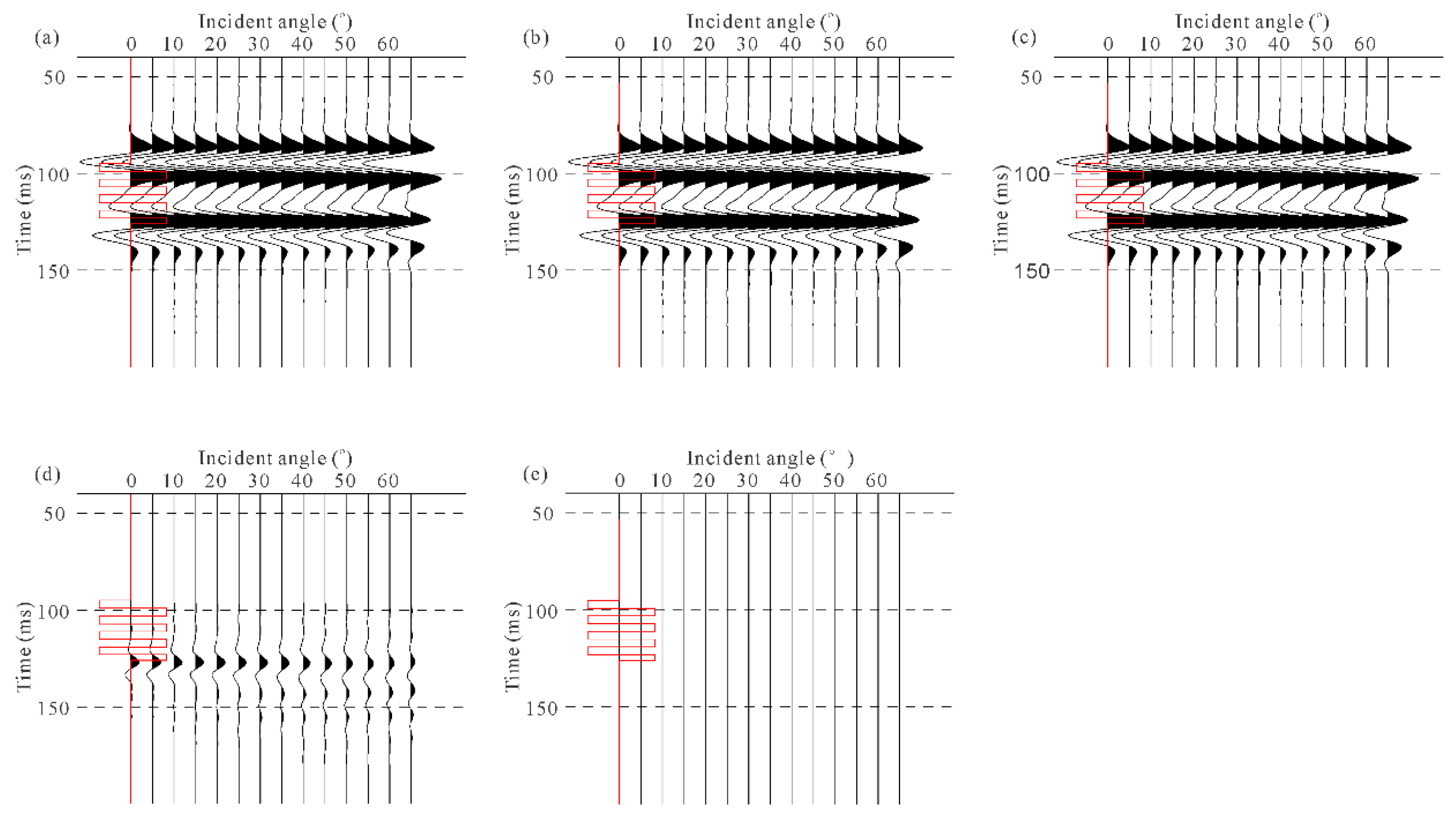
The second-order approximation equation effectively calculates the internal multiples (Figure 13d and Figure 14d), and these multiples are aliased together with the primary wave. It is difficult for existing technology to eliminate these internal multiples without affecting the energy of primary reflections.
(3)
As can be seen from Figure 13d and Figure 14d, for PP-waves, the internal multiples have a more significant effect on the reflection coefficient at small to medium angles, and the effect decreases as the incident angle increases. For PS-waves, the internal multiples have a large effect on the reflection coefficient at medium to large angles, and the effect becomes more significant as the incident angle increases.

4.3. Comparison With Field Multicomponent Data
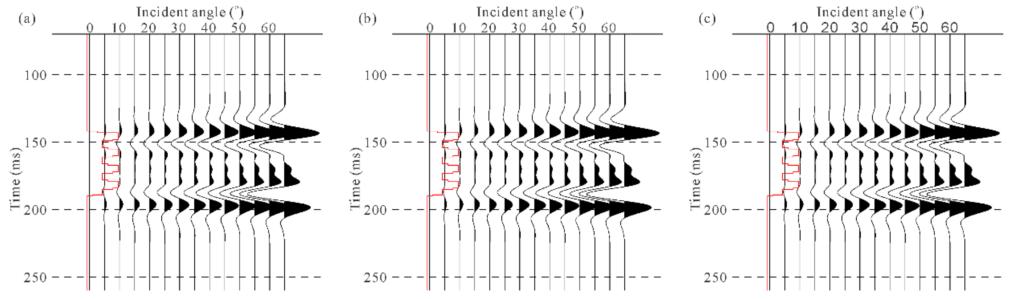
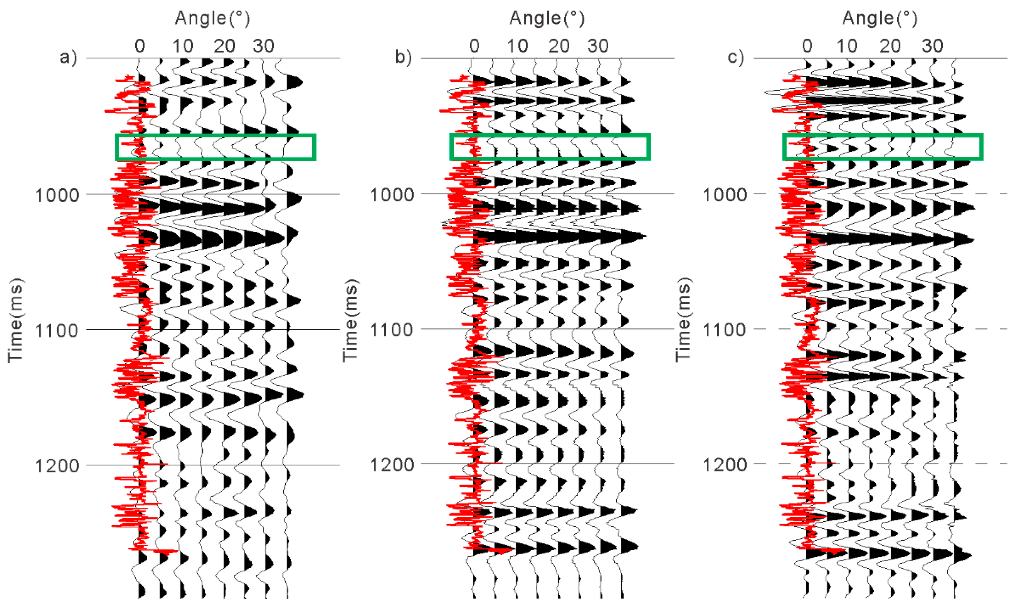
In order to verify the validity of the second-order approximate equation, we simulated the angle gather of field multicomponent data in the Sichuan Basin, West China [24]. Figure 15a and Figure 16a are the angle gather of field data at the well location for PP-wave and PS-wave, respectively. Besides, in order to compare the simulation accuracy, we simulated the angle gathers using exact Zoeppritz equations and second-order approximate equation. The seismic wavelets used for simulation are statistical wavelets extracted from the corresponding filed data [24]. Moreover, the simulation angle gathers are shown in Figure 15 and Figure 16. In summary, the comparison with field data reveals that:
(1)
The simulated angle gathers based on the second-order approximate equation will be more similar to the field data. For example, the field angle gather in the green box in Figure 15a has a phase inversion phenomenon, but this phenomenon only appears in the simulated angle gather based on the second-order approximate equation.
(2)
For thin interbeds, the simulation results of the second-order approximate equation contain richer information. As shown in Figure 16, the strata in the green box is thin interbeds. Moreover, the simulation results based on the second-order approximate equation contain internal multiples and are more similar to the field data.

5. Discussion

The reflection coefficient equations of the thin-bed and thin-interbed media discussed in this paper are approximated based on the Kennett equation. Our second-order approximate equations have no layer thickness limitation since there is no layer thickness limitation in the Kennett equation. For thick layers, multiples can be suppressed by the predictive deconvolution method. However, for thin-bed and thin-interbed layers, internal multiples are aliased together with primary waves, and it is difficult for the existing technologies to eliminate these internal multiples without affecting the energy of primary reflections. Therefore, for the inversion of a single thin bed and thin interbed, internal multiples must be considered, since this has a significant impact on the overall reflection coefficient.
During the analysis of the single thin-bed model, we found that if the impedance contrast is too large, the error of the approximate equation will increase. Therefore, the approximate equation of the thin-interbed is not suitable for strata with a large impedance contrast. Besides, although there are only two sets of interbed elements in thin-interbed model testing, the approximate equation can be applied to multiple sets of interbed elements.
We did not consider the influence of the incident angle during the derivation of the approximate equation. However, we found that the approximate equation of the PP-wave will have higher accuracy in the range of small and medium angles in the model tests. On the contrary, the approximate equation of the PS-wave can be applied to a broader range of incident angles. However, in order to cooperate with the PP-wave, we limited the application scope of the PS-wave approximation equation to the range of the PP-wave approximation equation. Most of the actual seismic data are acquired within a medium incident angle, because a large incidence angle tends to produce wide-angle reflections. In addition, the distortion caused by normal moveout correction is severe at large incident angles. Thus, reflections at large angles are often removed during data processing. Therefore, the second-order approximate equation is suitable for most seismic data.
The single thin-bed models and thin-interbed models can be divided into multiple types according to the strata parameters and thicknesses. The conclusions and phenomena we discussed above are only for the models involved in this paper. Therefore, there may be different phenomena in other models, which we will test in the future work.
Forward modeling using our equation is implemented in the frequency domain, and then the seismic record can be obtained by the conversion to the time domain. Thus, we should consider the time-frequency conversion when using our equations for AVO inversion, and the time consumption of this process is relatively large. In the next study, we will focus on designing a fast algorithm for our equation to improve the efficiency of AVO inversion.
In the numerical simulation analysis of the thin-interbed model, the thickness of each thin bed is set to a constant, and the elastic parameters of thin beds with the same lithology are also set to be consistent. Therefore, this model is idealized by us, but it does not affect the accuracy analysis of the second-order approximate reflection coefficient equations. The thickness of each thin bed in the actual thin-interbed strata is different, and the elastic parameters of thin beds with the same lithology may vary significantly. The anomalous seismic responses caused by the changes of physical properties of a thin bed in thin interbeds will be further studied in the future.

6. Conclusions

We analyzed the relationship between the energy of internal multiples and primary waves based on the single thin-bed model. Then, we proposed the second-order approximate reflection coefficient equations with a clear physical meaning for the single thin-bed model. For PP-waves, the approximate equation has a high accuracy at small to medium angles (≤30°), while for PS-waves, the equation can be applied to a larger range of angles. Under the assumption of weak impedance contrast, we extended the second-order approximate equation of the single thin-bed model to the thin-interbed model and tested its accuracy through numerical simulation analysis. At present, it is challenging to remove internal multiples in thin interbeds without affecting primary waves. In this case, the second-order approximate reflection coefficient equations can be used to calculate the total reflection coefficients of thin interbeds more conveniently and efficiently, which is conducive to improving the accuracy of seismic inversion.

Author Contributions

J.L. conceived the idea of this research. Z.Y. and J.L. deduced the equations. Z.Y. programmed the codes and performed the simulation tests. The paper was written by all the authors. All authors have read and agreed to the published version of the manuscript.

Funding

This research was funded by [National Natural Science Foundation of China] grant number [Nos U1910205 and 41574126].

Conflicts of Interest

This manuscript has not been published or presented elsewhere in part or in entirety and is not under consideration by another journal. We have read and understood your journal’s policies, and we believe that neither the manuscript nor the study violates any of these. There are no conflicts of interest to declare.

References

  1. Ostrander, W.J. Plane-wave reflection coefficients for gas sands at nonnormal angles of incidence. SEG Tech. Progr. Expand. Abstr. 1982, 216–218. [Google Scholar] [CrossRef]
  2. Ostrander, W.J. Plane-wave reflection coefficients for gas sands at non-normal angles of incidence. Geophysics 1984, 49, 1637–1648. [Google Scholar] [CrossRef]
  3. Hilterman, F.J. Seismic Amplitude Interpretation; SEG and EAGE: Houton, TX, USA, 2001; ISBN 1-56080-109-3. [Google Scholar]
  4. Lu, J.; Meng, X.; Wang, Y.; Yang, Z. Prediction of coal seam details and mining safety using multicomponent seismic data: A case history from China. Geophysics 2016, 81, B149–B165. [Google Scholar] [CrossRef]
  5. Xu, Z.; Tu, H.; Wu, Q. Reflection coefficient of planar wave and AVO technique. Geophys. Prospect. Pet. 1991, 30, 1–21. [Google Scholar]
  6. Pan, W.; Innanen, K.A. AVO/AVF analysis of thin-bed in elastic media. SEG Techn. Progr. Expand. Abstr. 2013, 373–377. [Google Scholar] [CrossRef]
  7. Yang, C.; Wang, Y.; Lu, J. Weak impedance difference approximations of thin-bed PP-wave reflection responses. J. Geophys. Eng. 2017, 14, 1010–1019. [Google Scholar] [CrossRef]
  8. Widess, M.B. How thin is a thin bed? Geophysics 1973, 38, 1176–1180. [Google Scholar] [CrossRef]
  9. Lu, J.M.; Wang, Y. The Principle of Seismic Exploration; China Petroleum University Press: Beijing, China, 2011; ISBN 978-7-5636-2822-3. [Google Scholar]
  10. Brekhovoskikh, L.M. Waves in Layered Media; Academic Process: Tamil Nadu, India, 1960. [Google Scholar]
  11. Brekhovskikh, L.M. Waves in Layered Media, 2nd ed.; Academic Press: New York, NY, USA, 1980; ISBN 0-12-130560-0. [Google Scholar]
  12. Kennett, B.L.N. Reflections, rays, and reverberations. Bull. Seismol. Soc. Am. 1974, 64, 1685–1696. [Google Scholar]
  13. Kennett, B.L.N. Seismic Wave Propagation in Stratified Media; Cambridge University Press: Cambridge, UK, 1983. [Google Scholar]
  14. Kennett, B.L.N. Seismic Wave Propagation in Stratified Media, 2nd ed.; ANUE Press: Canberra, Australia, 2009. [Google Scholar] [CrossRef]
  15. Liu, Y.; Schmitt, D.R. Amplitude and AVO responses of a single thin bed. Geophysics 2003, 68, 1161–1168. [Google Scholar] [CrossRef]
  16. Yang, C.; Wang, Y.; Wang, Y.H. Reflection and transmission coefficients of a thin bed. Geophysics 2016, 81, N31–N39. [Google Scholar] [CrossRef] [Green Version]
  17. Yang, C.; Wang, Y.; Lu, J.; Chen, B.C.; Shi, L. A Low-Order Series Approximation of Thin-Bed PP-Wave Reflections. Appl. Sci. 2019, 9, 709. [Google Scholar] [CrossRef] [Green Version]
  18. Lu, J.; Wang, Y.; Chen, J.; An, Y. Joint anisotropic amplitude variation with offset inversion of PP and PS seismic data. Geophysics 2018, 83, N31–N50. [Google Scholar] [CrossRef]
  19. Aki, K.; Richards, P.G. Quantitative Seismology, 2nd ed.; Integrated Book technology: Mill Valley, CA, USA, 2009; ISBN 978-1-891389-63-4. [Google Scholar]
  20. Mavko, G.; Mukerji, T.; Dvorkin, J. The Rock Physics Handbook: Tools for Seismic Analysis of Porous Media; Cambridge University Press: Cambridge, UK, 2009; ISBN -13. [Google Scholar]
  21. Fryer, G.J. A slowness approach to the reflectivity method of seismogram synthesis. Geophys. J. Int. 1980, 63, 747–758. [Google Scholar] [CrossRef] [Green Version]
  22. Castagna, J.P.; Batzle, M.L.; Kan, T.K. Rock physics—The link between rock properties and AVO response. In Offset-Dependent Reflectivity—Theory and Practice of AVO Analysis; Castagna, J.P., Backus, M., Eds.; Investigations in Geophysics, Society of Exploration Geophysicists: Tulsa, OK, USA, 1993; pp. 135–171. [Google Scholar]
  23. Gardner, G.H.F.; Gardner, L.W.; Gregory, A.R. Formation velocity and density—The diagnostic basics for stratigraphic traps. Geophysics 1974, 39, 770–780. [Google Scholar] [CrossRef] [Green Version]
  24. Lu, J.; Yang, Z.; Wang, Y.; Shi, Y. Joint PP and PS AVA seismic inversion using exact Zoeppritz equations. Geophysics 2015, 80, R239–R250. [Google Scholar] [CrossRef] [Green Version]
Figure 1. Schematic diagram of layered strata.
Energies 13 01465 g001
Figure 2. Schematic diagram of a single thin-bed model. r and t are the reflection and transmission coefficient matrices, respectively. Superscripts ‘(1)’ and ‘(2)’ denote the top and bottom interface of the single thin bed (Layer 2), respectively.
Energies 13 01465 g002
Figure 3. Reflected PP-wave modes in the thin-bed model. P- and S-wave paths are denoted by solid and dashed arrows, respectively.
Energies 13 01465 g003
Figure 4. Reflected PS-wave modes in the thin-bed model. P- and S-wave paths are denoted by solid and dashed arrows, respectively.
Energies 13 01465 g004
Figure 5. Energy ratios: (a) EM/EP, (b) EM1/EM, (c) EM2/EM, (d) EM3/EM.
Energies 13 01465 g005
Figure 6. Graphic representation of the second-order approximation equation (Equation (25)) of the reflection matrices for the single thin-bed model.
Energies 13 01465 g006
Figure 7. Angle gathers of PP-wave when ΔI = −1.5: (a) primary wave angle gather, (b) angle gather including first- and second-order multiples, (c) angle gather including all reverberations, (d) difference between b and a, (e) difference between c and d. The red curve donates the P-wave velocity.
Energies 13 01465 g007aEnergies 13 01465 g007b
Figure 8. Angle gathers of PS-wave when ΔI = −1.5: (a) primary wave angle gather, (b) angle gather including first- and second-order multiples, (c) angle gather including all reverberations, (d) difference between b and a, (e) difference between c and d. The red curve donates the S-wave velocity.
Energies 13 01465 g008
Figure 9. Ara variation with incident angle: (a) PP-wave, (b) PS-wave.
Energies 13 01465 g009
Figure 10. Accuracy analysis of the second-order approximate reflection coefficient of the PP-wave in the frequency domain: the modulus (a) and phase angle (b) of the second-order approximate reflection coefficient, the relative modulus error (c), and the relative phase error (d).
Energies 13 01465 g010
Figure 11. Accuracy analysis of the second-order approximate reflection coefficient of the PS-wave in the frequency domain: the modulus (a) and phase angle (b) of the second-order approximate reflection coefficient, the relative modulus error (c), and the relative phase error (d).
Energies 13 01465 g011aEnergies 13 01465 g011b
Figure 12. Schematic diagram of a thin-interbed model.
Energies 13 01465 g012
Figure 13. PP-wave angle gathers of thin-interbed model: (a) primary wave angle gather, (b) angle gather including first- and second-order multiples, (c) angle gather including all reverberations, (d) difference between b and a, (e) difference between c and d. The red curve donates the P-wave velocity.
Energies 13 01465 g013
Figure 14. PS-wave angle gathers of the thin-interbed model: (a) primary wave angle gather, (b) angle gather including first- and second-order multiples, (c) angle gather including all reverberations, (d) difference between b and a, (e) difference between c and d. The red curve donates the S-wave velocity.
Energies 13 01465 g014aEnergies 13 01465 g014b
Figure 15. PP-wave angle gathers of the field data in PP time domain: (a) field PP amplitude versus incident angle (AVA) data, (b) synthetic PP AVA data based on Zoepprotz equations, (c) synthetic PP AVA data based on the second-order approximate equation. The red curve donates the P-wave velocity log.
Energies 13 01465 g015
Figure 16. PS-wave angle gathers of the field data in PS time domain: (a) field PS AVA data, (b) synthetic PS AVA data based on Zoepprotz equations, (c) synthetic PS AVA data based on the second-order approximate equation. The red curve donates the S-wave velocity log.
Energies 13 01465 g016
Table 1. Parameters of the thin-bed model, where ΔI is the impedance contrast between the thin bed and its upper layer.
ΔI (km/s∙g/cm3)α2 (km/s)β2 (km/s)ρ2 (g/cm3)
54.8172.9812.579
4.54.6622.8462.558
44.5052.7112.536
3.54.3462.5742.514
34.1862.4372.490
2.54.0252.2982.466
23.8622.1572.441
1.53.6972.0152.414
13.5311.8712.386
0.53.3621.7262.357
−0.53.0181.4302.295
−12.8421.3712.261
−1.52.6641.2862.224
−22.4831.1982.185
−2.52.2981.1092.144
−32.1091.0192.098
−3.51.9160.9262.048
−41.7190.8311.993
Table 2. Elastic parameters of the thin-interbed model.
α (km/s)β (km/s)ρ (g/cm3)h (m)
3.0941.5152.400150
3.0481.5952.2306
3.1461.5542.4106
3.0481.5952.2306
3.1461.5542.4106
3.0481.5952.2306
3.1461.5542.4106
3.0481.5952.2306
3.1461.5542.4106
3.0941.5152.400150

