Study on Loose-Coupling Methods for Aircraft Thermal Anti-Icing System

Abstract

To simulate aircraft thermal anti-icing systems and solve the conjugate heat transfer of air-droplet flow and solid skin, the heat and mass transfer model of the runback water on the anti-icing surface was combined with the heat conduction equation of the skin by loosely coupled methods. According to the boundary conditions used for the runback water conservation equations, two loose-coupling methods for the heat exchange between the runback water and the solid skin were developed based on surface heat flow and surface temperature, respectively. The anti-icing and ice accretion results of a NACA 0012 electro-thermal anti-icing system were obtained by the two loose-coupling methods. The heat flow-based method directly solves the thermodynamic model of the runback water without any extra assumptions, but the convergence rate is relatively slow. On the other hand, the temperature-based method achieves higher calculation speed, but the freezing point is extended to an artificial temperature range between water and ice phases. When the value of the artificial temperature range is small, the results obtained by the temperature-based method are consistent with those of the heat flow-based method, indicating that the effect of freezing point extension can be ignored for thermal anti-icing simulation. Furthermore, the solutions of the two methods are in acceptable and comparable agreement with the experimental and simulative results in the literature, confirming their feasibility and effectiveness. In addition, it is found that the ice thicknesses and ice shapes rise obviously near the runback water limits as a result of the transverse heat conduction of the solid skin.

1. Introduction

When an aircraft flies in the cloud under icing conditions, its windward surfaces collect super-cooled water droplets, and ice accretion may occur [1]. Aircraft ice accretion has a significant effect on aircraft performances. It can cause increased drag, a decrease in lift and stall angle [2], and even lead to serious flight accidents [3]. Therefore, anti-icing or de-icing systems are usually equipped in aircrafts to protect critical surfaces and ensure flight safety [4].

Many kinds of ice protection devices have been developed, in which thermal anti-icing systems are traditional and the most prominent one used in modern aircrafts [5]. Currently, due to the low energy consumption, more and more attention has been paid to ice-phobic or super-hydrophobic coatings for aircraft ice protection. However, those coatings cannot prevent icing completely in practice, and they should be combined with thermal anti-icing systems to prevent ice formation [6]. In a thermal anti-icing system, the thermal energy provided by hot air [7] or electrical heaters [8] is conducted through aircraft skin to heat the protected surfaces and evaporate the impinging water droplets. When heating power density is insufficient to evaporate all the water droplets impinged on the local skin surface, a runback water film forms and flows backwards thanks to the aerodynamic forces [9]. The anti-icing characteristics depend not only on the air-water droplet flow parameters but also on the internal skin heat conductions. The anti-icing state can be divided into three categories according to the amount of energy applied [10]: (1) evaporative anti-icing: the impinging water evaporates in the heating area; (2) running wet anti-icing: the impinging water runs back behind the ice protected area, and freezes into ice ridges; (3) icing: the impinging water freezes with the anti-icing system turned off. To predict the temperature distribution on the anti-icing surface and analyze the system performances, a coupling method is necessary for the conjugate heat transfer of the external air flow, the internal skin heat conduction and the thermodynamics of the runback water on the aircraft surface. Unlike traditional conjugate heat transfer problems, the heat exchange between fluid and solid domains is affected by the runback water film when it flows backwards, evaporates, and freezes.

Since the effects of surface temperature and ice shape on external air flow and water droplet impact can be neglected, the convective heat transfer coefficient is assumed unchanged during the iteration process [11], and the anti-icing simulation is reduced to the coupled analysis of the runback water thermodynamics and the internal heat conduction. The heat transfer in the solid skin is generally determined by the thermal conduction differential equation, while the thermodynamic models of the runback water consist of Messinger [12], Meyer [13], Shallow water [14], rivulets [15], and so on. The coupling methods are critical for thermal anti-icing simulations to ensure the convergence of both temperature and heat flow at the runback water film-solid interface. Nearly all the ice accretion and anti-icing codes, such as LEWICE [16], FENSAP-ICE [17], ONERA [18], CANICE [19], and ICECREMO [20], use loose-coupling methods to perform the conjugate heat transfer solution [21]. Considering the runback water thermodynamics as an extra calculation domain, the loose-coupling method solves the control equations of the water film and solid domains individually to provide interface parameters for each other [22]. Exchanging boundary parameters continuously and iteratively, the solutions in both domains are carried out alternately until the temperature and heat flow in their interface converge. According to the parameters offered to the runback water equations, there are two loose-coupling methods: heat flow-based method and temperature-based one.

The heat flow-based method directly solves the thermodynamic model of the runback water under the condition that the heat flow at the water film-solid interface is known, and the calculation results are used as the boundary condition for the solid heat conduction equation, so as to update the heat flow of the interface to complete the conjugate heat transfer simulation. According to the parameters transferred between the water film and solid domains, various approaches, with different computational stabilities and convergences, have been established to implement the heat flow-based method for thermal anti-icing simulations. FENSAP-ICE [22] extracts the temperature at the water film-solid interface from solid heat conduction to calculate the surface heat flow with the help of a reference temperature and a local heat transfer coefficient. Then, the temperature solved by the thermodynamic model of the runback water is converted to a Robin boundary condition for the temperature update in the solid domain. By adopting the “improved Schwarz method,” Chauvin [23] took the same Fourier type boundary condition at the interface for both internal and external heat transfer calculations, and the surface heat flux was updated by its relationship with the temperature difference between the two adjacent domains. CANICE [19], Zhou [24] and Mu [25] directly used the surface heat flow from the solid heat conduction to solve the runback water equations, and the obtained temperature was taken as a Dirichlet boundary condition for the solid skin to update the interface heat flow.

On the other hand, the temperature-based method generally obtained the anti-icing heat load corresponding to the interface temperature by solving the conservation equations of the runback water film. The heat load is used as a Neumann boundary condition [26] or converted to a Robin boundary condition [27] for the solid skin to update its temperature field. However, when the surface temperature is at the freezing point, part of the runback water on the anti-icing surface freezes, but the ratio of ice to water is impossible to be determined under this temperature condition. LEWICE [16] assumes that water solidification occurs over a small artificial temperature range instead of at the freezing point, and then defines a freezing coefficient related with the temperature range between water and ice phases to calculate the heat load. Using the temperature-based method with this assumption, Domingos [28] simulated a hot-air anti-icing system, and Shen [29] calculated the temperature variations of an electro-thermal de-icing system. However, the influence of the freezing point extension on thermal anti-icing simulations has not been analyzed, and the value of the artificial temperature range has not been given in those articles, either.

At present, heat flow-based and temperature-based loose-coupling methods are widely used for thermal anti-icing simulation, and various implementation approaches have been developed. However, little attention has been paid to the comparisons and features of the two methods. With the same thermodynamic model of runback water and solid heat conduction equation, two loose-coupling methods are established based on anti-icing surface heat flow and surface temperature, respectively. The two methods are then used for the simulations of an electro-thermal anti-icing system under an evaporative anti-icing condition, a running wet anti-icing condition, and an icing condition to compare their characteristics and analyze the effect of the freezing point extension.

2. Heat and Mass Transfer Model

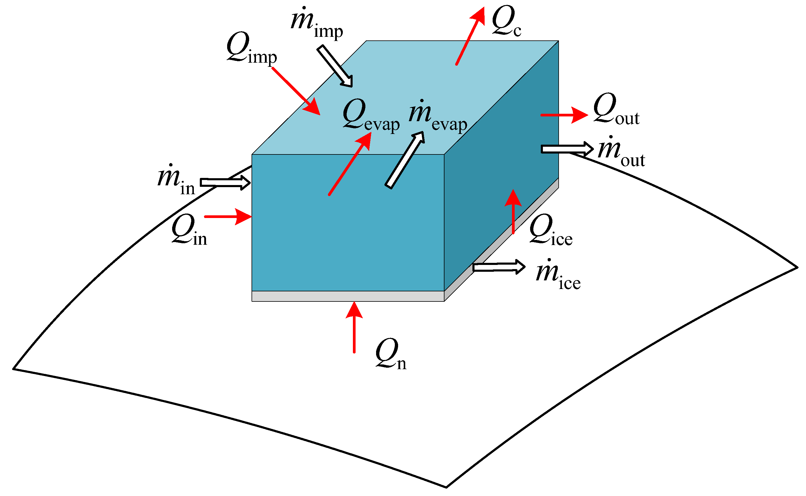
The runback water film, formed on the anti-icing surface after the impact of the super-cooled water droplets, is analyzed following the traditional Messinger [16] model. As shown in Figure 1, the mass flows in a control volume (CV) on the outer skin surface include: impinging water flow ${\dot{m}}_{\mathrm{imp}}$, evaporative water flow ${\dot{m}}_{\mathrm{evap}}$, and runback water flows entering ${\dot{m}}_{\mathrm{in}}$ and leaving ${\dot{m}}_{\mathrm{out}}$ the current CV. Correspondingly, the heat flows on the anti-icing surface consist of: heat flow brought by the impinging water droplets Q_imp, evaporative heat flow Q_evap, heat flows carried by the runback water inflow Q_in and outflow Q_out, convective heat flow of the external air Q_c, and heat flow conducted from the internal solid skin Q_n. When the heating power density is small and the anti-icing capacity of the thermal system is insufficient, ice accretion may occur on the outer skin surface, along with mass flow of the frozen water ${\dot{m}}_{\mathrm{ice}}$, and heat flow released by the frozen water Q_ice.

Thermal anti-icing is a steady heat and mass transfer process, and all the non-frozen water flows outwards of the current CV according to the Messinger model. Based on mass and energy conservation laws, we obtain the following equation [16]:

$$\{\begin{array}{c}{\dot{m}}_{\mathrm{imp}}+{\dot{m}}_{in}={\dot{m}}_{\mathrm{evap}}+{\dot{m}}_{\mathrm{out}}+{\dot{m}}_{\mathrm{ice}}\\ Q_{\mathrm{imp}}+Q_{\mathrm{in}}+Q_n+Q_{\mathrm{ice}}=Q_{\mathrm{evap}}+Q_{\mathrm{out}}+Q_c\end{array}$$

(1)

External air convective heat transfer is the only heat dissipating term when there is no water in the CV, and the heat flow can be calculated by the convective heat transfer coefficient h_s and the temperature difference between skin surface and air [29]:

$$Q_c=h_s\cdot \left(T_s-T_{\mathrm{ad}}\right)\cdot \Delta s$$

(2)

where T_s is the surface temperature, T_ad is the reference surface temperature calculated by the airflow solver based on an adiabatic boundary condition, and Δs is surface length of the CV.

The motions of the super-cooled water droplets can be calculated with the help of the Lagrangian or Eulerian method, and the impinging water flow is obtained by:

$${\dot{m}}_{\mathrm{imp}}=\beta \cdot U_{\infty }\cdot LWC\cdot \Delta s$$

(3)

where β is the local collection efficiency and LWC is the liquid water content.

With the assumption that the enthalpy of the liquid water at the freezing point is zero, the heat flow brought by the impinging water droplets is obtained by:

$$Q_{\mathrm{imp}}={\dot{m}}_{\mathrm{imp}}\cdot \left[\frac{U_{\infty }^2}{2}+c_{p,w}\cdot \left(T_{\infty }-T_{\mathrm{ref}}\right)\right]$$

(4)

where T_ref is the freezing point temperature, 273.15 K.

When dry air flows through wet surface, diffusion process of water molecules occurs under the concentration difference, and the evaporative water flow can be obtained by the Chilton-Colburn analogy theory [23]:

$${\dot{m}}_{\mathrm{evap}}=\Delta s\cdot \frac{h_s}{c_{p,\mathrm{air}}}\cdot {\left(\frac{Pr}{Sc}\right)}^{\frac{2}{3}}\cdot \frac{M_v}{M_{\mathrm{air}}}\cdot \left[\frac{p_{v,\mathrm{sat}}\left(T_s\right)-p_{\mathrm{v},\mathrm{e}}}{p_e-p_{\mathrm{v},\mathrm{e}}}\right]$$

(5)

where p_v,sat(T_s) is the saturated evaporative pressure at the surface temperature T_s [21].

At the same time, the heat flow taken away by the evaporative water is:

$$\{\begin{array}{l}{Q}_{\mathrm{evap}}={\dot{m}}_{\mathrm{evap}}\cdot \left[i_{\mathrm{sv}}+c_{p,\mathrm{ice}}\cdot \left(T_s-T_{\mathrm{ref}}\right)-i_{\mathrm{ls}}\right]\hspace{0.17em}\hspace{0.17em}{T}_s<T_{\mathrm{ref}}\\ Q_{\mathrm{evap}}={\dot{m}}_{\mathrm{evap}}\cdot \left[i_{\mathrm{lv}}+c_{p,w}\cdot \left(T_s-T_{\mathrm{ref}}\right)\right]\hspace{0.17em}\hspace{0.17em}\hspace{0.17em}{T}_s\ge T_{\mathrm{ref}}\end{array}$$

(6)

In addition, the heat flow released by the frozen water includes the latent heat and the sensible heat:

$$Q_{\mathrm{ice}}={\dot{m}}_{\mathrm{ice}}\cdot \left[i_{\mathrm{ls}}+c_{p,\mathrm{ice}}\cdot \left(T_{\mathrm{ref}}-T_s\right)\right]$$

(7)

Lastly, the sensible heat flows carried by the runback water can be written as:

$$Q_{\mathrm{in}}={\dot{m}}_{\mathrm{in}}\cdot c_{p,w}\cdot \left(T_{in}-T_{\mathrm{ref}}\right)$$

(8)

$$Q_{out}={\dot{m}}_{out}\cdot c_{p,w}\cdot \left(T_s-T_{\mathrm{ref}}\right)$$

(9)

For the CV at the stagnation point, no runback water enters, and ${\dot{m}}_{\mathrm{in}}=0$. For other CVs, the amount of the inflow water is equal to the vale leaving the upstream CV. Therefore, the solution of the runback water is performed from the stagnation point backwards along either side so that ${\dot{m}}_{in}$ is a known quantity at each location [16]. However, there are four unknowns, T_s, Q_n, ${\dot{m}}_{\mathrm{out}}$, and ${\dot{m}}_{\mathrm{ice}}$, in the two conservation equations for a CV on the anti-icing surface. Two additional conditions are needed to close the heat and mass transfer model. One should be the parameter provided by the adjacent solid skin domain, and the other is the constraint between the freezing point and the phase state of runback water.

3. Coupling Methods and Solution Procedures

As described in the Introduction, the calculations of the external air-droplet flow and the air convective heat transfer coefficient were separated from the coupled analysis of the runback water thermodynamics and the solid skin heat conduction. In this paper, the external air flow and temperature fields were obtained by Reynolds-averaged Navier-Stokes equations (RANS) with the Spalart-Allmaras (S-A) turbulence model. An ideal gas was defined for the external air. The pressure-far-field boundary condition was used for the airflow inlet, while no slip wall was set for the anti-icing surface. The maximum value of y+ in the anti-icing area was about 0.3, which satisfies the S-A model requirement of y+ < 1 for boundary layer calculation. Moreover, the mesh independence was satisfied for convective heat transfer coefficients, and the check procedure was the same as that in the reference [30]. The air flow and water droplet motion were considered to be one-way coupled, ignoring the influence of droplet on airflow field, and an Eulerian method [31] was used to get the local water droplet collection efficiency.

With the external air and water droplet results, the loose coupling method was adopted to perform the conjugate heat transfer solution of thermal anti-icing system. The runback water thermodynamic model was coupled with the heat transfer in the solid skin, and the heat conduction differential equation in the skin can be written as:

$$\rho c_p\frac{\partial T}{\partial t}=\nabla \cdot \left(\lambda \nabla T\right)+S$$

(10)

To solve this equation, the boundary condition of the outer skin surface was needed, and could be obtained by the thermodynamic model of the runback water. Due to the parameters offered to the heat and mass transfer equations of the runback water, the two loose-coupling methods below were developed with different solution procedures.

3.1. Heat Flow-Based Coupling Method

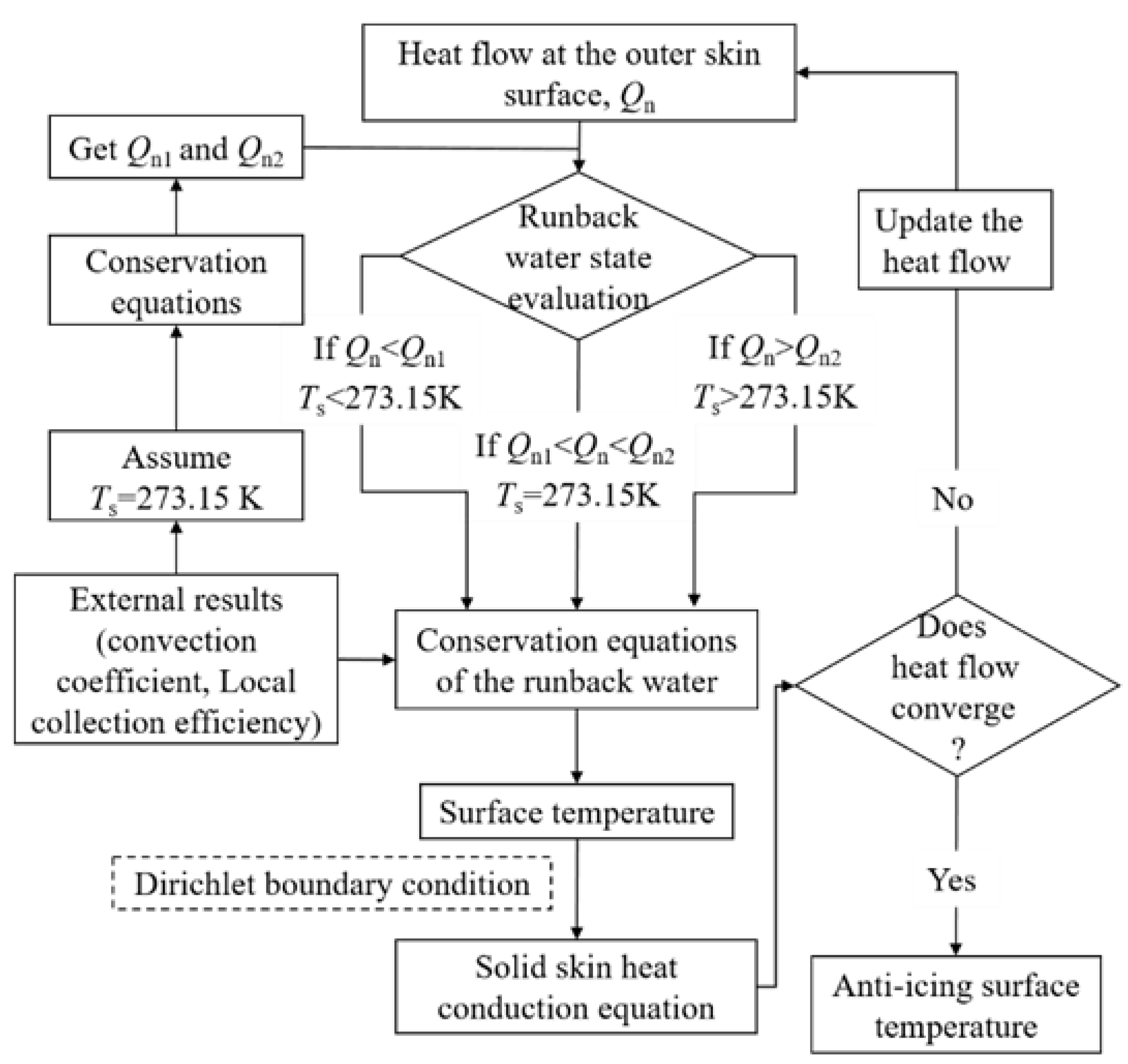
Since heating power is transferred to the outer skin surface for ice protection in a thermal anti-icing system, the surface heat flow Q_n can be obtained from the temperature field of the solid skin to solve the runback water conservation equations; the surface temperature was taken as a Dirichlet boundary condition of the heat conduction equation to update the skin temperature field and the surface heat flow. In this heat flow-based coupling method, the constraint between the surface temperature and solid-liquid phase state can be expressed as follows: (1) When Q_n is large enough, the anti-icing surface temperature is higher than the freezing point, and there is no ice layer accumulated (${\dot{m}}_{\mathrm{ice}}=0$); (2) When Q_n is small, its temperature is lower than the freezing point, and the water is completely frozen with no runback water flowing out (${\dot{m}}_{\mathrm{out}}=0$); (3) Otherwise, the surface temperature is at the exact freezing point under moderate heat flow, and the mass flow of the frozen water can be determined by Q_n. With this constraint, the unknowns in the runback water equations are reduced to two, and the solution is unique.

However, it can be seen that the mass and energy conservation equations are implicit functions when surface temperature is solved by the heat flow-based coupling method. It is difficult to identify the solid-liquid phase state during the iterative solution of the implicit functions. To avoid computational divergence, the surface heat flow Q_n is evaluated to predetermine the water phase state before the runback water solution, as shown in Figure 2. With the surface temperature set to 273.15 K, the critical heat flows under which all water freezes and all water remains liquid were calculated, respectively [24]. When all water freezes at 273.15 K, the corresponding heat flow Q_n1 is the critical point that the ice layer begins to melt, which can be obtained by:

$$\{\begin{array}{c}{\dot{m}}_{\mathrm{ice}}={\dot{m}}_{\mathrm{imp}}+{\dot{m}}_{in}-{\dot{m}}_{\mathrm{evap}}\\ Q_{\mathrm{n}1}=Q_c+Q_{\mathrm{evap}}-Q_{\mathrm{imp}}-Q_{\mathrm{in}}-Q_{\mathrm{ice}}\end{array}$$

(11)

When all water remains liquid at 273.15 K, the corresponding heat flow Q_n2 is the critical value corresponding to when the liquid water begins to freeze, which can be calculated by:

$$\{\begin{array}{c}{\dot{m}}_{\mathrm{out}}={\dot{m}}_{\mathrm{imp}}+{\dot{m}}_{in}-{\dot{m}}_{\mathrm{evap}}\\ Q_{\mathrm{n}2}=Q_c+Q_{\mathrm{evap}}+Q_{\mathrm{out}}-Q_{\mathrm{imp}}-Q_{\mathrm{in}}\end{array}$$

(12)

For a specific heat flow Q_n transferred from the solid heat conduction, the water phase state can be determined by comparing these two critical heat flows: If $Q_{\mathrm{n}}>Q_{\mathrm{n}2}$, the heat flow is large with no water freezing, and T_s > 273.15 K; If $Q_{\mathrm{n}}<Q_{\mathrm{n}1}$, the heat flow is small and T_s < 273.15 K, leading all the water to freeze; If $Q_{\mathrm{n}1}<Q_{\mathrm{n}}<Q_{\mathrm{n}2}$, water and ice coexist on the surface, and T_s = 273.15 K. Then, the thermodynamic model of the runback water is solved separately. During the iterations between the runback water and the solid skin, the corresponding surface temperature is regarded to be the final thermal anti-icing temperature when the deviation of the surface heat flow is small enough. The solution procedure of this heat flow-based coupling method is presented in Figure 2.

3.2. Temperature-Based Coupling Method

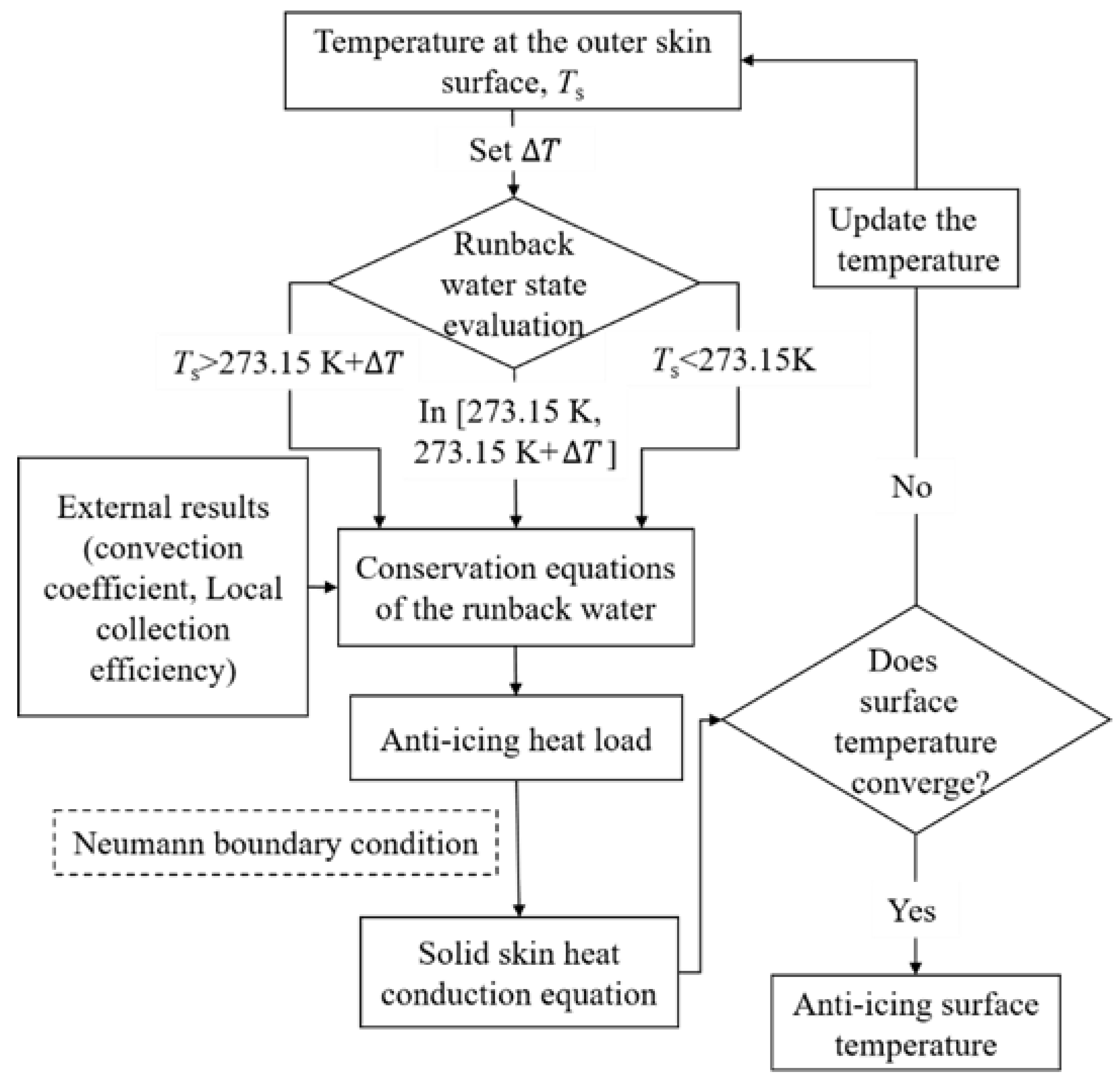
Assuming that the thermal anti-icing system meets the anti-icing temperature requirement, the mass and energy conservation equations of the runback water can be solved according to the known surface temperature, and the corresponding anti-icing heat load can be obtained according to this surface temperature. Then, the heat load is taken as a Neumann boundary condition for the solid skin, and the anti-icing surface temperature can be updated by solving the heat conduction differential equation. Calculation converges when the temperature deviation between the iterations reaches a very small value. This coupling method extracts the anti-icing surface temperature T_s to calculate the runback water model, and is called the temperature-based coupling method.

Since the surface temperature is known in this method, the solid-liquid phase state can be determined directly. When T_s > 273.15 K, there is no icing, and ${\dot{m}}_{\mathrm{ice}}=0$. Moreover, when T_s < 273.15 K, the surface water is completely frozen; thus, there is no water flowing out of the CV, and ${\dot{m}}_{\mathrm{out}}=0$. In both conditions, two unknowns can be reduced for the conservation equations, and the heat and mass transfer model of runback water can be solved to obtain the anti-icing heat load. In addition, since heat load is an explicit function of temperature, the solution of the mass and energy conservation equations is performed without iteration, resulting in little calculation time.

However, when T_s = 273.15 K, part of the runback water freezes, and there are still three unknowns, Q_n, ${\dot{m}}_{\mathrm{out}}$, and ${\dot{m}}_{\mathrm{ice}}$, in the two equations. It can be explained that the ratio of ice to water in the CV is impossible to be determined at the surface temperature of 273.15 K, so that the anti-icing heat load cannot be obtained. Under this circumstance, the phase transformation process of the runback water is regarded to occur within an artificial temperature range ΔT, instead of at the exact freezing point [16]. With this assumption, the freezing point temperature is extended from 273.15 K to the water-ice mush zone [273.15 K, 273.15 K+ΔT].

The frozen water in the CV is defined as the freezing coefficient f, as expressed as:

$$f=\frac{{\dot{m}}_{\mathrm{ice}}}{{\dot{m}}_{in}+{\dot{m}}_{\mathrm{imp}}-{\dot{m}}_{\mathrm{evap}}}$$

(13)

Following the approaches of LEWICE [16] and Domingos [28], f is related to ΔT:

$$f=1-\frac{T_s-T_{ref}}{\mathsf{\Delta }T}$$

(14)

Then, the equations to be solved for the mush zone become:

$$\{\begin{array}{c}{Q}_{\mathrm{imp}}+Q_{\mathrm{in}}+Q_n+Q_{\mathrm{ice}}=Q_{\mathrm{evap}}+Q_{\mathrm{out}}+Q_c\\ {\dot{m}}_{in}+{\dot{m}}_{\mathrm{imp}}={\dot{m}}_{\mathrm{evap}}+{\dot{m}}_{\mathrm{out}}+{\dot{m}}_{\mathrm{ice}}\\ {\dot{m}}_{ice}\cdot \Delta T=\left({\dot{m}}_{in}+{\dot{m}}_{\mathrm{imp}}-{\dot{m}}_{\mathrm{evap}}\right)\left(T_{ref}-T_s+\Delta T\right)\end{array}$$

(15)

Consequently, the temperature range above the freezing point becomes T_s > 273.15 K + ΔT, and the anti-icing heat load at any surface temperature can be obtained by the method of explicit functions. The solution process of the runback water model and the specific procedure of the temperature-based coupling method are presented in Figure 3.

Since the surface temperature corresponds to the heat flow on a one-to-one basis without any extra assumptions in the heat flow-based coupling method, its results fully satisfy the conversation equations of runback water and the solid heat conduction equation, and its solution is considered to be accurate. To study the effect of the freezing point extension, the results of the temperature-based coupling method are compared with those of the temperature-based one. In addition, the parameter of the artificial temperature range ΔT between water and ice phases is analyzed in this work, and the values of 0.01 K, 0.1 K, and 1 K are used for the simulations in the temperature-based method.

4. Geometry and Conditions

To focus on the anti-icing coupling methods, an electro-thermal anti-icing system of NACA 0012 airfoil is chosen for numerical simulations. The experimental results of the system can be found in the reference [10], and these have been used to validate many anti-icing codes. Case 22A and Case 22B were chosen for anti-icing calculations. Despite sharing the same external airflow and water droplet conditions, Case 22A is an evaporative anti-icing condition under which the water droplet totally evaporates in the ice protected area, while Case 22B is a running-wet anti-icing condition and the runback water would turn into ice on the skin surface after flowing out of the heated zone. Spray time was defined for Case 22B to obtain the runback ice shape. In addition, an icing condition with the anti-icing system turned off was also analyzed, in which the chord length is different from that under the anti-icing conditions. The external conditions of Run 401 were selected from the reference [32] for the icing simulation. The specific parameters relating to external air flow and water droplet motion for all three cases are listed in

Table 1. External airflow and icing conditions.

	Case 22A	Case 22B	Run 401
Chord length, m	0.9144	0.9144	0.5334
U∞, m/s	44.7	44.7	102.8
T∞, °C	−7.6	−7.6	−7.78
LWC, g/m3	0.78	0.78	0.55
Diameter, μm	20	20	20
Angle of attack, °	0	0	3.5
Spray time, s	/	420	420

.

The thermal anti-icing system was attached to the leading edge to protect the windward surface, since the water droplets usually impact there. Seven heating elements were arranged along the chord direction inside the skin, as shown in Figure 4. The heating power of each element can be controlled individually.

Table 2. Position and heat flux of the heating element.

Heating Element	Start_s/c	End_s/c	Heat Flux, kW/m2
			Case 22A	Case 22B	Run 401
F	−0.1024	−0.0607	9.92	2.635	0
D	−0.0607	−0.0329	10.23	2.945
B	−0.0329	−0.0051	32.5	4.03
A	−0.0051	0.0157	46.5	4.805
C	0.0157	0.0435	18.6	2.945
E	0.0435	0.0713	6.98	3.41
G	0.0713	0.1129	10.24	2.325

lists the specific position and heat flux for each electrical heating element, where the dimensionless surface distance s/c is measured from the leading edge of the airfoil. The value of s/c is negative on the lower surface and positive on the upper one.

As can be seen from Figure 4, the solid skin is composed of six layers, and the material properties of the multi-layered structure are listed in

Table 3. Material properties of the multilayer skin [10].

Material	λ, W/m/K	ρ, kg/m3	cp, J/kg/K	Thickness, mm
Heating Element (alloy 90)	41.018	8906.26	385.112	0.0127
Erosion Shield (SS 301 HH)	16.269	8025.25	502.32	0.2032
Elastomer (COX 4300)	0.256	1383.99	1255.8	0.2794
Fiberglass/Epoxy Composite	0.294	1794.07	1569.75	0.889
Silicone Foam Insulation	0.121	648.75	1130.22	3.429

. The thickness of each layer presented in the table is the value when the chord length is 0.9144 m, and it changes proportionally for Run 401. The thickness and thermal resistance of the outer skin are small, while those of the inner skin are large. Therefore, most of the electrical energy is conducted outwards for anti-icing, and the inner surface of the solid skin can be set to be adiabatic.

5. Result and Discussion

5.1. Results of Case 22A

Local water droplet collection efficiency β of the NACA 0012 airfoil obtained by the Eulerian method is presented in Figure 5 for Case 22A. It can be seen that the β value used in this paper agrees well with those of ANTICE [10] and Silva [8]. Overall, the collection efficiency gradually decreased as the distance to the leading edge increased, with a maximum value of about 0.56 located at the stagnation point. The positions of the impingement limits were around s/c = ±0.32, which means the droplet impingement range was within the ice-protected area.

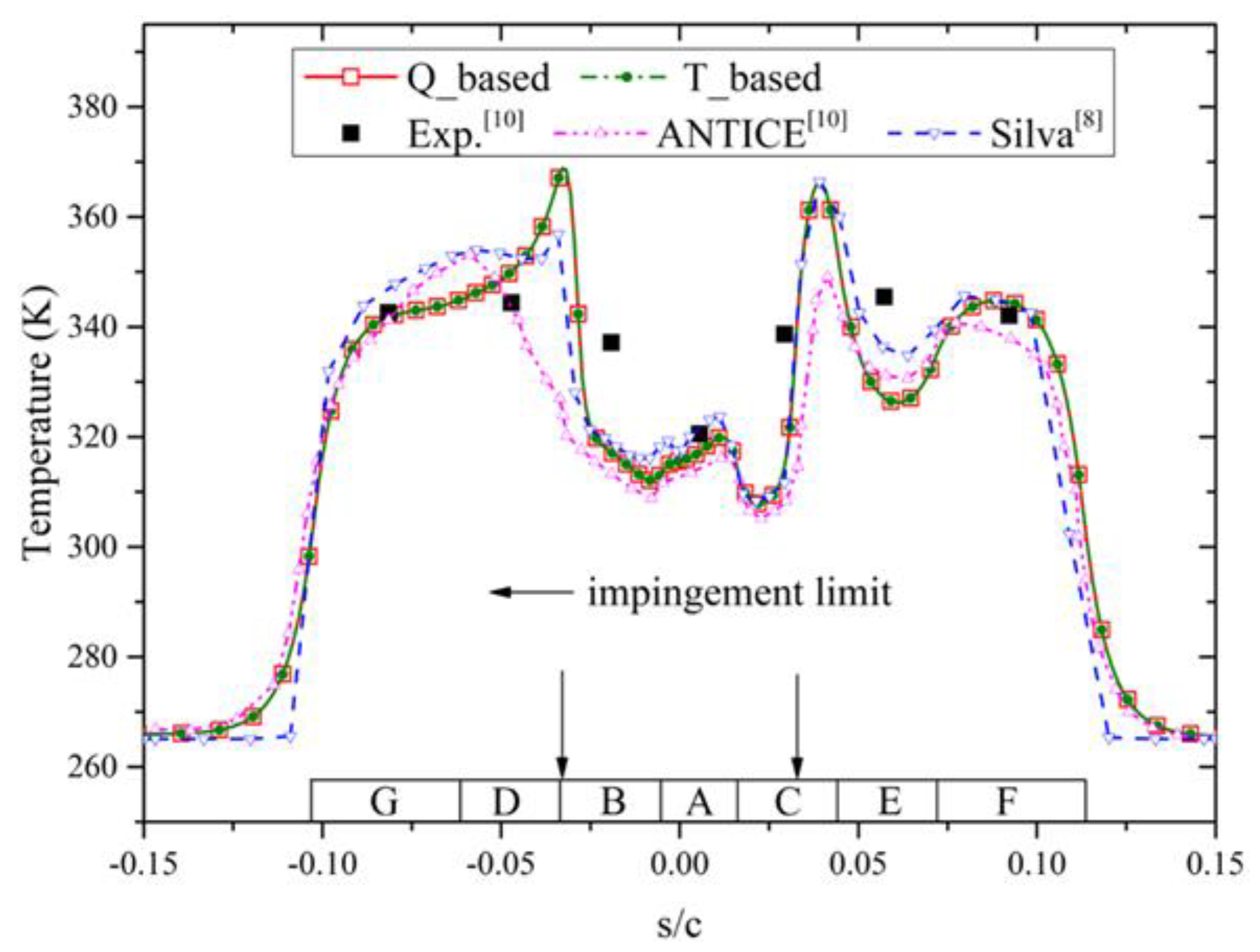
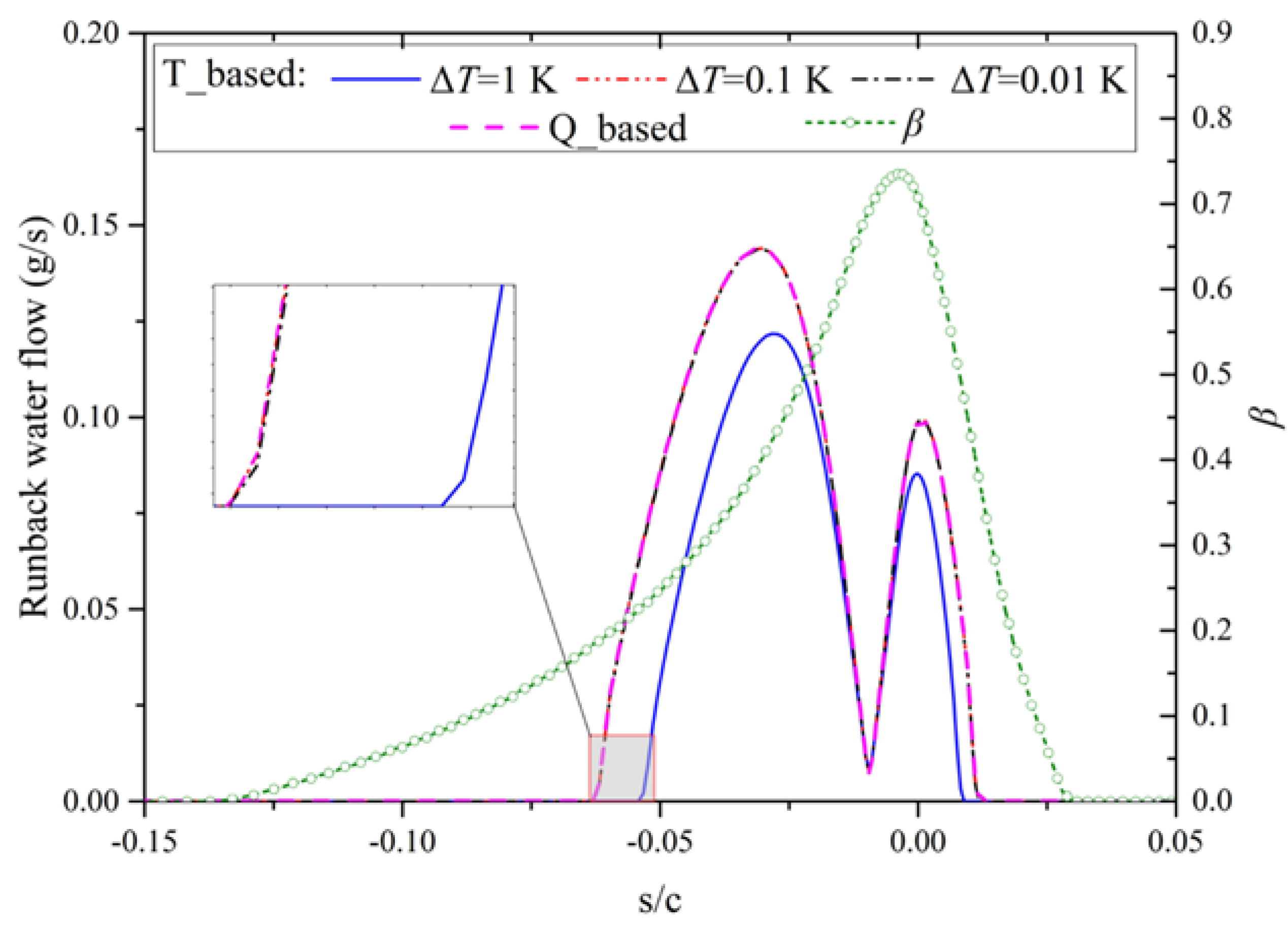
The runback water flow on the external skin surface and the surface temperature distribution for Case 22A are presented in Figure 6 and Figure 7, respectively. Since the temperatures of runback water were all above the freezing point under this evaporative anti-icing condition, the results at ΔT = 0.01 K, 0.1 K and 1 K are the same in the temperature-based coupling method, and only one curve is shown in the figure. It can be seen from Figure 6 that the runback water flow was low at the stagnation point, and the value gradually increased, peaking at s/c of around 0.022 and −0.015 on the upper and lower surfaces, respectively. The runback water flow finally declined to zero when all the water in the CV evaporated. In addition, the control volumes bearing the runback water were all within the water droplet impingement region, which indicates that Case 22A was a totally evaporative anti-icing condition. Figure 7 shows that, due to the heat flow taken away by the water evaporation, the temperature near the stagnation point was low in spite of the large electric heat flux. When there is no water in the CV, the surface temperature rose rapidly, and remained at a high value until the edges of the heated area.

Furthermore, the results of the runback water flow and surface temperature solved by the heat flow-based coupling method were almost identical to those obtained by the temperature-based one, since the two methods solve the same water flow equations without the effect of the freezing point extension in this case. The curves of both methods match well with the data in literatures as evidence for the feasibility and accuracy of the two coupling methods for evaporative anti-icing conditions.

5.2. Results of Case 22B

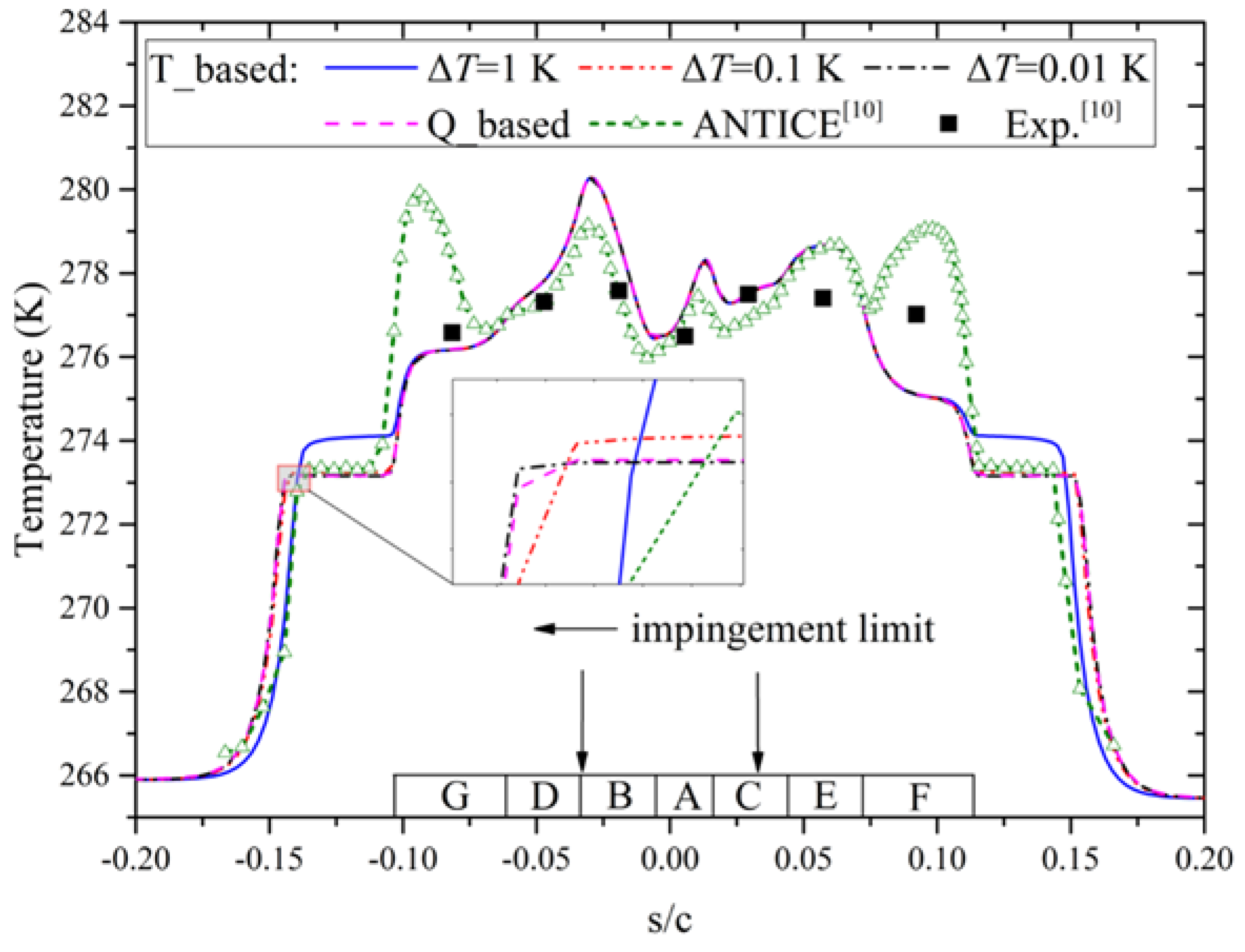
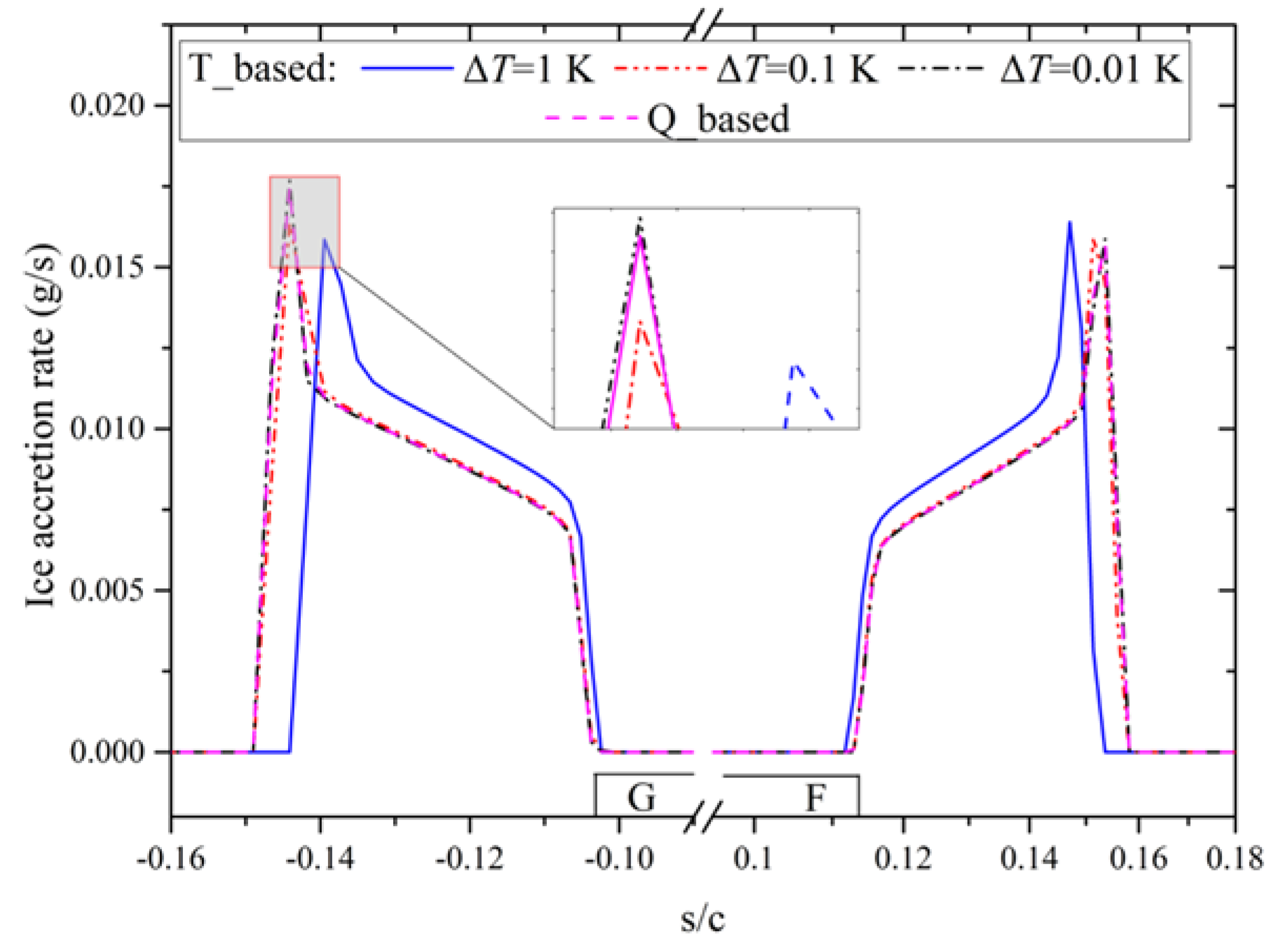
Figure 8, Figure 9, and Figure 10 present the runback water flow, the temperature distribution, and the ice accretion rate on the anti-icing surface for Case 22B, respectively. The runback water film flows backwards along the upper and lower surfaces from the stagnation point, and the liquid water exists in the whole ice protected area since it is a running-wet anti-icing condition. Due to the electric power loaded around the leading edge, the temperature is relatively high and fluctuates with the heat fluxes of the heaters in the heated area. When the surface temperature drops to the freezing point outside this region, part of the runback water begins to freeze, and the runback water flow drops quickly. The surface temperature remains stable at the freezing point or in the range from 273.15 K to 273.15 K + ΔT as it moves backwards, and it drops when the water is totally frozen. This type of icing is caused by the runback water and refers to the glaze ice ridge. Around the water film end positions, the calculated ice accretion rate increased sharply to form two obvious rises, which was due to the heat removed through the conduction of solid skin.

When ΔT = 0.01 K in the temperature-based coupling method, the runback water flow, surface temperature, and ice accretion rate outside the heated area are in good agreement with those of the heat flow-based coupling method, indicating that the effects of the freezing point extension can be neglected with low ΔT. Additionally, the anti-icing results obtained by the two coupling methods show satisfactory numerical accuracy on comparison with the literature data, verifying the feasibility and accuracy of both methods for running-wet anti-icing conditions. As the value of ΔT increases in the temperature-based method, the deviations go up as a result of higher phase changing point, and the errors are significant at ΔT = 1 K.

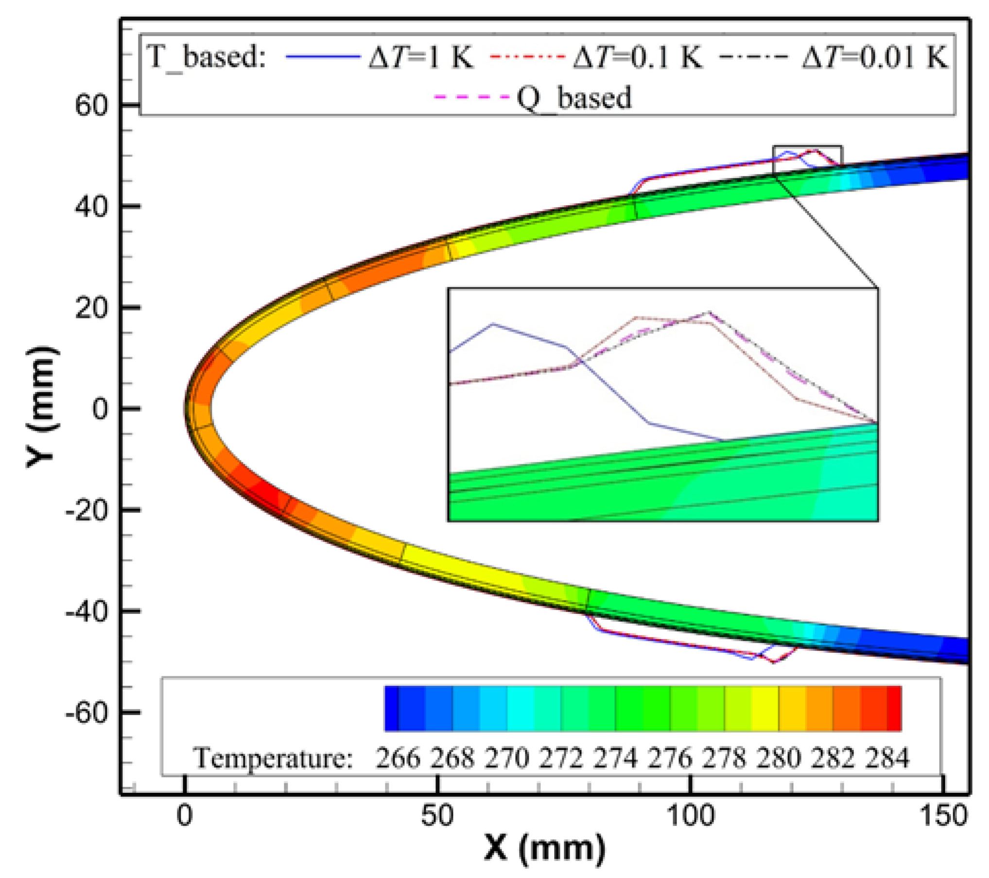
Following the approach of Ref. [2], the ice shape can be obtained based on the ice accretion rate. Figure 11 show the ice shape of Case 22B, along with the contour of the skin temperature obtained by the heat flow-based method. There was no ice accreted on the heated area, and the skin temperature varied with the heat fluxes of the heaters. The temperature decreased to the freezing point around the ends of the protected area, and an ice layer began to form on the surface. The differences of the ice shapes obtained by the two methods were small, except when ΔT = 1 K. Near the ends of the icing area, the ice thicknesses were relatively large with a high ice accretion rate, which was also found by Morency [33]. As shown in Figure 11, the temperature differences in the transverse direction were quite large near the ends of the icing area, so that extra heat flow was taken away to the downstream region by the heat conduction of the solid skin, and more water froze there to form peaks.

5.3. Results of Run 401

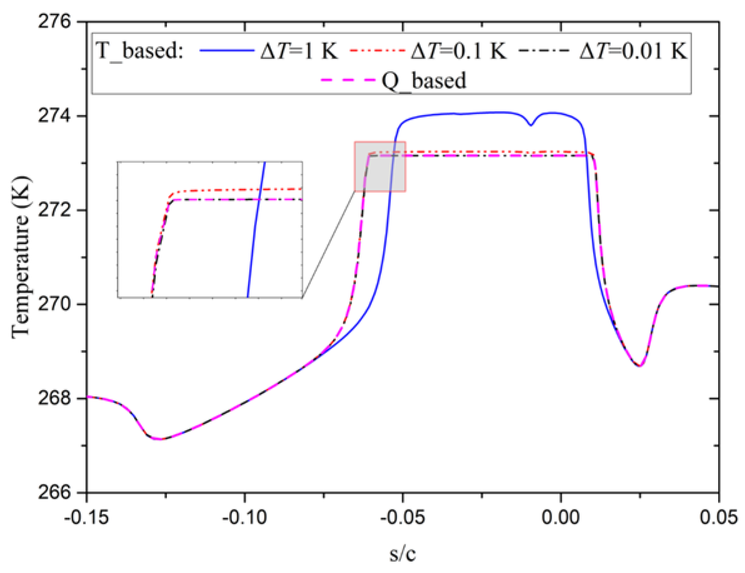
The runback water flow results of Run 401 are presented in Figure 12, along with the local water droplet collection efficiency. Because the stagnation point was located on the lower airfoil surface due to positive angle of attack, a larger droplet impingement range existed on the lower surface. The runback water distributed around the stagnation point, and the ice accreted in this area was glaze ice. The runback water flow declined to zero when it moved backwards, and the droplet impingement range was larger than the runback water range. In the droplet impingement range, no runback water on the icing surface means that the water droplets froze instantaneously when impinging; this is the rime ice area. Therefore, the icing type of Run 401 was mixed ice, since glaze ice and rime ice coexisted on the skin surface. As shown in Figure 13, the surface temperature in the glaze ice area keeps at the freezing point or in the range of 273.15 K ~ 273.15 K + ΔT, and when it changed to rime ice, the temperature dropped rapidly below that. When the temperature-based coupling method was applied, the phase change temperature at ΔT = 1 K was relatively high, leading to noticeable deviations in terms of runback water flow and surface temperature. The calculated results, however, match well with each other when ΔT was 0.01 K and 0.1 K. Moreover, there were no noticeable differences observed between the heat flow-based coupling method and the temperature-based one with a low value of ΔT.

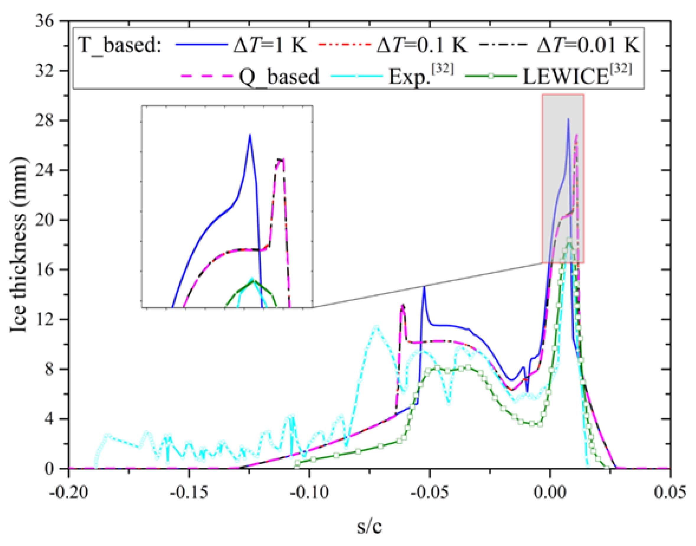
The ice thickness distribution and ice shape for Run 401 are presented in Figure 14 and Figure 15, respectively. The ice thickness was initially small at the stagnation point on the lower airfoil surface, and then grew to form ice horns as the distance to the stagnation point increased. In the rime ice area, it decreased smoothly, and reached zero at the droplet impingement limits. When the ice type transitioned from glaze ice to rime ice, the ice thickness has obvious rises with the peaks in ice shape curves near the end positions of the runback water, which is the same as the situation in Case 22B but different from the result obtained by the traditional method of LEWICE [32]. LEWICE did not consider the heat conduction in solid skin. As can be seen from the temperature distribution obtained by the heat flow-based method in Figure 15, the latent heat flow released by water freezing keeps the skin temperature above the ambient value. Since surface temperature in the glaze ice area was near the freezing point, the skin temperature was relatively high near the stagnation point. As the amount of freezing water flow decreased, the latent heat released can be taken away immediately by the airflow convection, resulting in the skin temperature dropping rapidly in the rime ice area. Therefore, a large temperature difference in the transverse direction lies between the glaze ice and rime ice areas, and extra latent heat released by water freezing can be removed through solid skin easily, resulting in a peak of ice thickness there. Furthermore, the icing results obtained by the heat flow-based and temperature-based coupling methods were in comparable agreement with the experimental and simulative data in the literature as evidence of the applicability for icing conditions.

5.4. Comparison of Computational Time

In order to guarantee the convergence and stability in solving the complex conjugate heat transfer problem, the relaxation coefficient was used for both loose-coupling methods. Since the numerical instability and the under-relaxation scheme were not studied in detail in this work, the comparison of computational time was qualitatively analyzed for the two methods. It was found that the relaxation coefficient can be relatively large, and the convergence rate was fast for the temperature-based method. Even in the case of the runback water freezing in which a small relaxation coefficient was used due to small value of ΔT, its calculation converged more quickly (about 20 min) than that of the heat flow-based one (about 1 h). This might be attributed to two reasons, as follows.

Firstly, the heat flow-based method needs an iterative process to solve the implicit functions of the heat and mass transfer conservation equations of the runback water, while the solution of the temperature-based method can be obtained directly from the explicit functions.

Secondly, there was an effect of the interface boundary condition on the convergence speed of solid heat conduction. When the Dirichlet boundary condition was used, the boundary temperature updated during coupling iteration would lead to the redistributions of heat flow and temperature in the whole solid region. If the temperature changes dramatically, divergence occurred. Therefore, a very small relaxation coefficient was required and the convergence was slow for the method based on surface heat flow. On the other hand, when Neumann boundary condition was applied for the solid heat conduction, the effect of the heat flow change on the anti-icing surface could be limited in a small range by the transverse heat conduction. Thus, a larger relaxation coefficient can be taken to accelerate the convergence speed in the temperature-based coupling method.

6. Conclusions

Two loose-coupling methods, heat flow-based and temperature-based, were established to simulate aircraft thermal anti-icing systems. Numerical calculations are performed for a NACA 0012 electro-thermal anti-icing system under the conditions of evaporative anti-icing (Case 22A), running wet anti-icing (Case 22B) and icing (Run 401). The main conclusions are as follows:

(1) When the artificial temperature range between water and ice phases is small (ΔT ≤ 0.1 K), the results obtained by the temperature-based method are consistent with those of the heat flow-based one, indicating that the effect of freezing point extension can be ignored.

(2) The anti-icing and icing results obtained by both coupling methods are in acceptable and comparable agreement with the experimental and simulative results in the literature, verifying the feasibility and effectiveness of the methods.

(3) Due to the transverse heat conduction of the aircraft skin, there are obvious rises of ice accretion rate and ice shape around the ends of the runback water range.

(4) Compared to the heat flow-based coupling method, the temperature-based one has faster computational speed, and its solution can converge with higher relaxation coefficient.