Article

Systematic Frequency and Statistical Analysis Approach to Identify Different Gas–Liquid Flow Patterns Using Two Electrodes Capacitance Sensor: Experimental Evaluations

by
Fayez M. Al-Alweet
1,2,*,
Artur J. Jaworski
3,*,
Yusif A. Alghamdi
4,5,*,
Zeyad Almutairi
4,6 and
Jerzy Kołłątaj
7
1
National Center for Oil and Gas Technology, King Abdulaziz City for Science and Technology, P.O. Box 6086, Riyadh 11442, Saudi Arabia
2
National Center for Corrosion Technology, King Abdulaziz City for Science and Technology, P.O. Box 6086, Riyadh 11442, Saudi Arabia
3
School of Computing and Engineering, University of Huddersfield, Huddersfield HD1 3DH, UK
4
Sustainable Energy Technologies Center (SET), King Saud University, P.O. Box 800, Riyadh 11421, Saudi Arabia
5
Deanship of Scientific Research (DSR), King Saud University, Riyadh 11421, Saudi Arabia
6
Mechanical Engineering Department, King Saud University, P.O. Box 800, Riyadh 11421, Saudi Arabia
7
Department of Electrical Engineering, Białystok Technical University, Wiejska 45D, 15-351 Białystok, Poland
*
Authors to whom correspondence should be addressed.
Energies 2020, 13(11), 2932; https://doi.org/10.3390/en13112932
Submission received: 26 April 2020 / Revised: 23 May 2020 / Accepted: 2 June 2020 / Published: 8 June 2020
(This article belongs to the Special Issue Fluid Flow and Heat Transfer Ⅱ)

Abstract

:
This work proposes a method to distinguish between various flow patterns in a multiphase gas–liquid system. The complete discrimination between different flow patterns can be achieved by mapping the corresponding frequency and statistical parameters. These parameters are usually obtained from further analysis conducted on the signal data of the utilized sensor. The proposed technique is based on establishing interrelationships between these parameters, namely the mean (m), the standard deviation ( σ ¯ ), power spectral density (PSD), the width of the characteristic frequency peaks (Δƒ), the skewness ( γ 1 ) and the kurtosis ( γ 2 ). Therefore, a relatively simple electrical capacitance sensor with two electrodes was designed and implemented on a two-phase flow apparatus with a circular pipe. The experimental operating conditions comprised of different combinations of air–water superficial velocities at three inclinations (i.e., horizontal, upward 15° and upward 30°). This research discusses in specific the analysis underlying flow patterns identification method and the rationale for selecting the proposed approach. The results showed that some parameters found to be more valuable than others such as m, σ ¯ and Δƒ. Besides, combining two sets of these statistical graphs which are (a) σ ¯ vs. Δƒ with Δƒ vs. m (or Δƒ vs. total power), (b) Δƒ vs. total power with γ 1 vs. σ ¯ (or γ 2 vs. σ ¯ ), and (c) σ ¯ vs. m with Δƒ vs. m (or Δƒ vs. total power), allowed all flow patterns field to be identified clearly at all inclinations. It is therefore concluded that for any gas–liquid multiphase flow system, the reported approach can be used reliably to discriminate between different generated flow patterns.

1. Introduction

1.1. Multiphase Flow Systems

A wide ranges of interfaces are possible in a system that depends on two types of flow (i.e., multiphase system: gas–liquid flow, gas–solids flow, or liquid–solids flow), due to the exceptionally great quantity of flow formations inside the pipe or the fluidized bed. These interfaces and flow formations manifest themselves as the typical flow regimes or patterns [1,2,3]. In addition, there are three significant features of those multiphase flow systems, which are (a) the flow regimes/patterns, (b) liquid/gas/solids holdup (including its time-dependent holdup fluctuations), and (c) pressure drop (including its time-dependent pressure fluctuations). These characteristics, especially the holdup and the pressure fluctuation, are largely influenced by the generated hydrodynamic of the system and its corresponding flow patterns/regimes. Henceforth, the developed hydrodynamic status is a crucial characteristic of any multiphase flow system. A strong comprehension and correctly predicting the generated flow are tremendously essential for many multiphase flow aspects, such as the pipelines/fluidized-bed design, calculating pressure-drop/holdup, and for numerical studies. However, it is very difficult and complex to estimate and compute multiphase flow discrete phenomena due to the artefact of several variables. These variables are the heat and mass transfer, and the interfaces present among any two types of phases and its corresponding slippage [4,5,6]. Moreover, there are many operating variables that can affect the hydrodynamics of a multiphase flow system such as (1) the pipe cross sectional area and arrangement, (2) superficial velocities, (3) direction and angle of inclination, and (4) the physical features of the utilized fluids and particles (solids size, liquid/gas/solids density, liquid/gas viscosity and the surface tension) [7,8,9,10,11]. The focus of this study will be on the gas–liquid multiphase flow system. Generally, in the research literature, several different flow patterns in the horizontal flow are observed. These flow patterns are discrete bubbles, elongated bubbles, slug, slug-churn, annular, and stratified flow, except plug flow [9,10]. In the upward flow inclination, all the abovementioned flow patterns are observed including plug except stratified flow pattern [10,12], whereas in the downward flow inclination, due to the gravity effect, only stratified flow is observed [10]. Therefore, the real time prediction and distinguishing between all flow patterns by the utilization of measurement devices are very significant. This can support engineers in the industrial field and academic researchers to calculate and optimize the hydrodynamics status, the variables of the system, and predict the generated flow patterns.

1.2. Flow Patterns Identification Techniques

There are many well investigated techniques for identifying the flow patterns [10,13,14,15,16,17,18,19,20,21,22,23,24,25,26]. Researchers in the field have used image post-processing methods to (a) categorize different flow formations and (b) measure the intermittent flow pattern velocities [13,14,15,27]. High speed camera images were usually used to study the rise of an air bubble and its generated field in a still liquid, and therefore, discriminate between different flow patterns by using an active photochromic dye technique [28]. Others also suggested this method to measure the size/shape of the bubbles as well as calculating the bubble rising velocity [6,29]. Such approach can be only accurate and valid for low flow rate operating conditions. This is because at high superficial velocity, the flow becomes more chaotic and even if the flow pattern can be identified, however, the flow velocity is more difficult to calculate. The main advantage of image post-processing methods is that they can positively differentiate among all the flow regimes. Yet, the implementation of image post-processing method in the actual multiphase system is expensive, time consuming and difficult to use in the industry.
Other techniques which were developed for multiphase flow pattern identification are the electrical capacitance [10,20,22,25,30,31], optical fiber probes [32], hot film anemometers [33], and conductive probes [6,34,35,36,37]. The focus and the approach explored in the current study is on the electrical capacitance technique. The electrical capacitance sensor is suitable because it provides values of the phase’s field and distribution around the pipe cross-section (or core visualization), gives an instantaneous distribution of the flow pattern, and measures the gas/liquid holdup [9,10,17,18,19,20,22,23,25,26,30,31,36,38].
A typical electrical capacitance sensor comprises of two to sixteen electrodes around the circumference of a pipe, parted by small gaps. The capacitor and its signal are usually influenced by the disturbance of the electromagnetic fields inside the pipe and the linking wires of the utilized electrodes. The factors affecting the signal can be reduced through optimizing the capacitor shield and reducing the connecting wire as much as applicable [39]. It was reported that the accurate visual formation obtained from a capacitance sensor is influenced by the size and the number of the electrodes. In addition, by minimizing the area between the electrodes, the ratio of the capacitance value to its produced noise can be fundamentally reduced. Thus, a proportional relation was observed between the sensitivity of the capacitor and the electrodes’ conduct region, indicating that the measurements of the electrical capacitance that were captured from all potential pairs of electrodes can provide a method to reconstruct images of the electrical filed generated by any flow pattern inside the pipe.
Many inherent disadvantages were observed when a tomography method was used [17,24], (1) the distortion of the reconstructed images, (2) a high acquisition system for the measured data is required, and (3) to capture and reconstruct representative visualization from blaring and distorted data, an instantaneous iteration method is also required. The measurement system of electrical capacitance sensors (with more than two electrodes) is typically comprised of a purpose-built multiplexer, an effective resistance analyzer (or impedance) and a processer with a monitor to reconstruct the images [26]. A capacitor comes in many arrangements such as a plate with double helix configuration, multiple helixes, four concave plates, circular shape capacitors, parallel plates, and concave or staggered concave plates [10,16,40]. The performance of the capacitance depend on many factors, including (a) the electrode length [21], (b) the shape and the quantity of the electrodes [16,38], (c) the capacitor insulator structure, (d) the physical conditions of the medium inside the pipe (including the temperature of the fluid/gas), and (e) the unwanted stray capacitance due to the wire connection between the capacitance to the multiplexer [20,41]. In addition, many different studies that were conducted on capacitance sensors concluded that the accurateness of the capacitance measurements is high when the relation between the length of the electrode (Le) and the pipe outer diameter (dout) was Le/dout ≥ 1 [18,23]. Most of the recent studies investigated the performance of more than two electrodes, however, such configuration is expensive and requires regular calibration and other related equipment as mentioned above.
For a concave two electrodes capacitance, Elkow et al. (1996) conducted a performance-based comparison study on two capacitance sensors which are a concave plate and a helical plate. They reported that the helical sensors had many disadvantages, including irregular response, reduced sensitivity and degraded shielding. However, all these limitations can be eliminated by the utilization of a concave capacitor [19]. The accuracy and sensitivity of the concave capacitor with two electrodes can be improved by designing the electrodes to have the same length. Thus, the irregularity of the produced electrical field is reduced, and the nonlinearity of the measurement is removed [19]. In addition, a couple of measures and configurations can be applied to eliminate the stray of the capacitance produced by the communication between its electronic components including: (1) making the space between the capacitor’s electrodes and its shield large enough, (2) also this distance has to be relative to the parting length between the electrodes of the capacitance sensor [36]. Stott et al. (1985) compared between an internal and external concave two electrodes sensor in a multiphase flow system. It was concluded that the external capacitance prediction was within 10% of the experimental results and higher than that of the internal capacitance [42]. Additionally, a specific advantage of the two electrodes capacitance is that it is very sensitive to low gas concentration in comparison to the available options such as gravimetric and nucleonic instruments. In addition, it can be used for both gas/liquid concentration measurements, however, with some limitations [16,43]. It must be noted that the concave two electrodes sensor suffers from lower resolution when compared to more than two electrode sensors; it cannot construct tomography images (as known tomography images cannot be obtained with less than eight electrodes [17,24]), and it has high uncertainty in void fraction measurement (i.e., especially for post-intermittent flow regimes) when comparted with sensors that have more than two electrodes [44,45]. These limitations of the two electrodes capacitance were also observed by Beck et al. (1985) and described in their work. They stated that such capacitance can only be utilized to determine the gas holdup in a system with less than 15% gas concentration when it was tested on a horizontal test section [43]. This is understandable since it is well known that such capacitance could not accurately measure the gas/liquid concentration [44,45]. However, it can be very useful for time-dependent signal fluctuation analysis in identifying different generated flow patterns [16,45,46,47].
Early work by Gerates and Borst (1988) stated that two electrodes cannot detect local void fraction with high accuracy for mixed flow patterns. This is because the flow patterns at the higher end of the intermittent flows are characterized by frothy slugs and a comparatively lengthy axial extension of the flow pattern. Accordingly, high uncertainty in void fraction predictions are observed. However, it can successfully be used for flow pattern identification if further analysis is conducted on the time-dependent output signal of the capacitance [45]. Later, Canière et al. (2008) utilized a two electrodes capacitance sensor which was tested on a small diameter pipe on a horizontal multiphase flow setup. The time-dependent output values, along with its resultant variance and frequency, were found to be very useful for conducting further analysis and can be used as a flow pattern detection tool [47]. In another recent work, Salehi et al. (2017) stated that if the main aim of using the capacitance is only the measurement of gas/liquid holdup, the ring-shaped capacitance is favored. On the other hand, for flow patterns detection, capacitance with a concave shape (such as that of two electrodes) is ideal, owing to its high sensitivity to the generated flow patterns [46]. There are many solid research works used and have validated the usefulness of such sensors in multiphase flow [16,17,19,21,24,42,43,44,45,46,47,48,49] for time-dependent single fluctuation (capacitance or voltage values) to identify different flow patterns. However, these studies are limited in inclinations and in the tested range of the experimental variables (i.e., the range of gas–liquid superficial velocities). Therefore, additional investigation is necessary to shed a light on the usefulness of a simple two electrode capacitance for flow pattern detection in term of frequency and statistical analysis.

1.3. Frequency and Statistical Analysis

Enhanced understanding of a multiphase flow in gas–liquid or gas–solids system for flow pattern/regimes classifications can be achieved by performing a systematic investigation on the frequency and statistical data. These frequency and statistical data can be obtained from one of the following time-dependent signals: (1) the capacitance signal [50,51], (2) gas/liquid void fraction signals [52], (3) pressure fluctuation signals [51,53,54], (4) impedance probes and non-intrusive sensors [55,56], and (5) optical method [51]. These statistical parameters which were captured from the instantaneous signals are the mean (m), standard deviation ( σ ¯ ), skewness ( γ 1 ) and kurtosis ( γ 2 ) [53,54]. In a gas–solids two-phase flow, Bai et al. (1996) considered the conventional pressure sensors and its time-dependent fluctuations in a fluidized bed with single riser to characterize various fluidization regimes. They stated that the solids volume fraction and its fluctuation correspond to a certain regime which reflects the status of the system [57]. In addition, Leu and Wu (2000) used the standard deviation ( σ ¯ ) obtained from the fluctuations of the pressure to estimate the minimum superficial velocity of mixed fluidized bed [58]. Also, the combustion region in a gas–solids fluidized bed can be determined by further analysis of the pressure signals [59].
In a gas–liquid multiphase flow system, it was found that distinguishing between different flow patterns can be achieved by capturing the variation of the output signal as a function of time. The typically used parameters are the output of the signal, the power spectral densities (PSD), histograms, and probability density functions (PDF) [50,51]. In addition, due to the complex phenomena observed in gas–liquid systems, the hydrodynamics of such systems can be additionally investigated by the useful information extracted from the PSD dominant values that were obtained from fast Fourier transform (FFT) technique [2]. This is because a non-linearity is observed in the processed signals as a function of time owing to the nonstationary nature and locally induced status of the system hydrodynamics [53,60,61,62]. Keska and Wiliams (1999) studied the effect of different measurement techniques (i.e., two electrodes capacitive signals, pressure signals, and optical method) and their abilities to identify different flow patterns from bubble to churn flow [51]. They used the output signals, PDF and the cumulative PDF (CPDF) as parameters in their comparative analysis. For flow pattern detection, it was found that each investigated measurement sensor showed different ability and potentiality to identify the generated flow patterns. In general, the pressure sensor proved to be lower in potential when compared with the capacitance sensor. Also, the optical method capability was limited and can only be used for narrow ranges of gas concentration (applicable only for above 70% liquid concentration) [51].
This study will propose a new approach to distinguish between different flow patterns in a two-phase gas–liquid system by using the data obtained from a capacitance sensor and mapping its corresponding frequency and statistical parameters. The basis of the proposed approach relies on the generated flow patterns, its corresponding measured capacitance values, and the interrelation between them. A relatively simple two electrodes capacitance device (concave-shaped) was designed and later implemented on a two-phase flow apparatus with a circular pipe using different combinations of gas–liquid superficial velocities at three inclinations (i.e., 0°, 15° and 30°). The paper will discuss in particular the experimental setup, the measurement principle underlying the identification method, and the significance of the related frequency and statistical parameters, which will help to discriminate between various flow patterns.

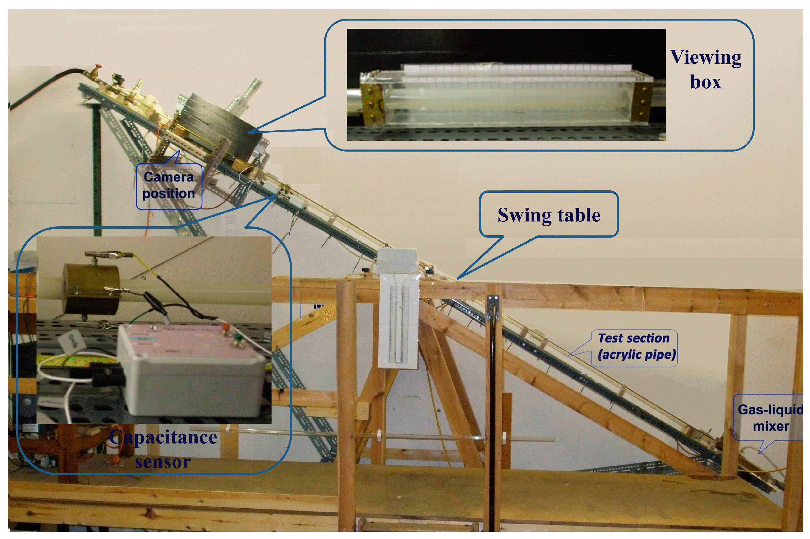
2. Experimental Apparatus and Methodology

A multiphase gas–liquid flow experimental apparatus was built to study the typically generated flow patterns (located at the University of Manchester). The apparatus was 4.0 m long, built from a transparent acrylic pipe with an inner diameter (din) of 20.0 mm, which allowed for the observation of the flow’s internal hydrodynamic status [9]. Additionally, a rectangular shaped box filled with water was used, as shown in Figure 1. This transparent viewing box helped to minimize the misrepresentation of the captured images to study the flow patterns. In addition, it worked as a cooling medium against the effect of the heat produced by the illumination system used with the utilized high-speed camera. The flow patterns were identified and characterized by the images captured from the NAC 500 Analogue High Speed Video system (nac Image Technology, Simi Valley, CA 93065 USA). To allow all flow patterns inside the pipe to be fully established hydrodynamically, it was important to capture the high-speed images at the right distance. This distance was estimated to be about 3.4 m from the pipe inlet. The recording duration of the high-speed camera was set to 2 min. The speed of the shutter was at 1/10,000 s, while the captured images frame rate was at 500 frames/s. The flow loop was built as a recirculating multiphase flow system, which was an appropriate configuration to guarantee good mixing between the phases and permit the development of various flow patterns. Two flexible elbow pipes and appropriate support of the test section enabled changing the inclination between 0° and 30°. The rig was designed to operate with water flow rates up to 75.0 L/min (i.e., 0 to 1.06 m/s increased gradually at equal intervals of 0.106 m/s) and air flow rate up to 96 L/min (i.e., 0 to 5.0 m/s increased gradually at equal intervals of 0.25 m/s).
The gas phase was delivered at room temperature from an in-house air compressor system. For the supplied gas phase (air), a pressure valve along with a metering system were utilized to deliver the air at a constant and stable flow rate. The liquid phase was pumped by a centrifugal pump from the water reservoir at room temperature and at atmospheric pressure via a regulator to sustain stable and continuous water flow rate. A manual valve was used to control a soft pipe that was used to recirculate the excess water back to the reservoir. Several pressure and temperature measuring instruments were fitted on the pipe which helped to monitor the flow hydrodynamic conditions. Additionally, to measure the supplied liquid flow rate, a turbine flowmeter was used in the setup. Before and during the operating of each experimental case, the liquid phase temperature was measured for the two tanks by two thermometers (one located at each tank). This is because it was important to keep all the experimental operating conditions constant, especially the liquid temperature (maintained approximately at 20 °C). A phases mixer was installed in the apparatus just before the inlet of the test pipe. The job of this mixer was to allow good mixing between the used gas and liquid phases (air and water). The mixer comprised of two different size pipes within each other: (a) the external and larger one was an acrylic Perspex pipe, and (b) the internal and smaller one was a brass pipe with perforations distributed on its boundary in a staggered shape. Thus, such configuration for the brass pipe guaranteed smooth entry of the air into the mixer system from the gap existing in between, due to the difference in diameter between the two pipes. The liquid phase will be delivered through the axial direction in the annulus of the pipe. Hence, a good mixing was achieved just before the inlet of the test pipe.
All the experimental cases studied in this work are presented in terms of operational maps that identify and distinguish between the observed flow patterns. The maps were constructed based on the combined effect and interrelation between the superficial air and water velocities, where each developed pattern was distinguished by a different color and symbol. Each developed flow pattern shown in Figure 2 was categorized by a visual investigation and the recorded images. The operating maps developed in this work are presented in Figure 2; they show the defined flow patterns and the transition between them for all the examined inclinations (horizontal, upward 15° and upward 30°). Altering the pipe angle influenced the manifestation of different flow patterns and the transition boundaries between them. In the horizontal case, all the patterns were observed except for plug flow, while for both upward angles, all patterns were distinguished except stratified flow pattern [9,10]. The liquid holdup was measured by using two fast closing valves [10]. As demonstrated in Figure 2, the air superficial velocities influenced the generated flow patterns and their corresponding liquid holdup. It is shown that as the gas superficial velocity increases, the corresponding liquid holdup decreases.

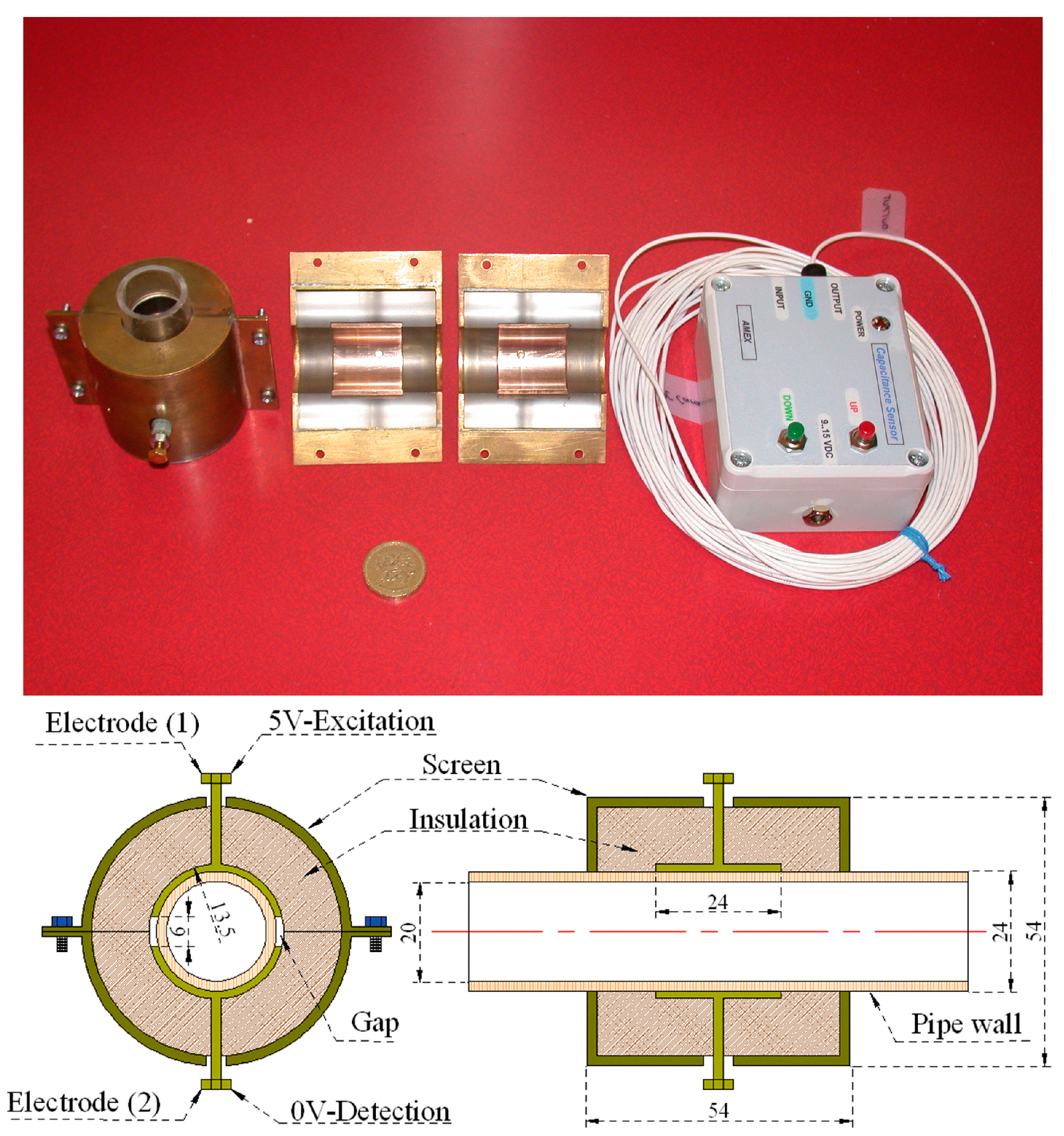
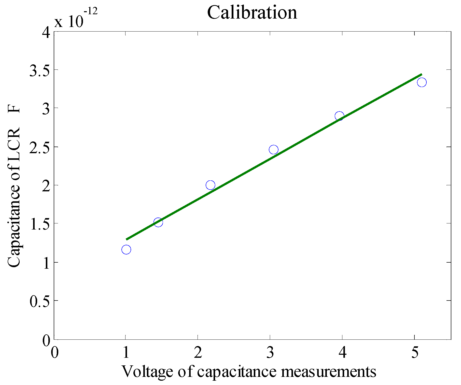
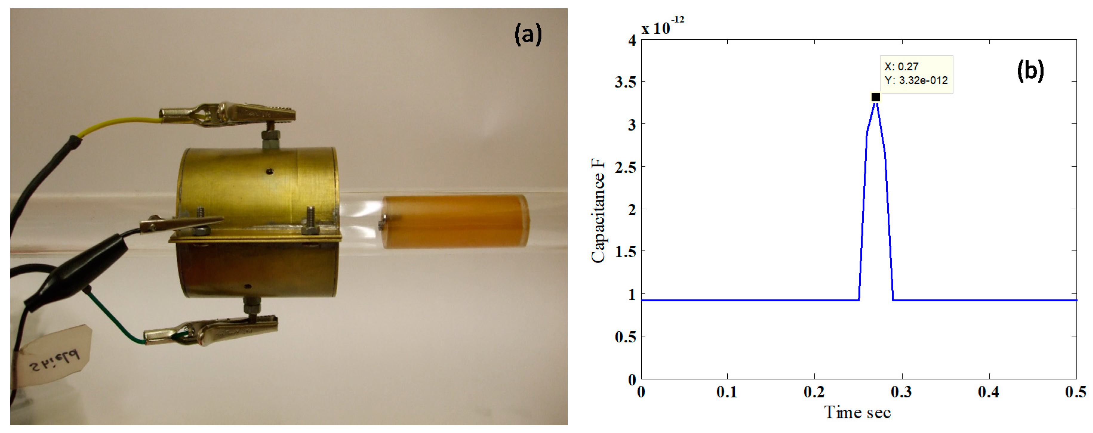
2.1. Two Electrodes Capacitance

The capacitance sensor was designed to consists of two equal separate parts, as shown in Figure 3; such a design allowed the sensor to be easily attached on the test pipe. Therefore, the fabricated two electrodes were fastened on the pipe’s external circumference and opposite to each other. Two important design factors were taken into consideration to support the sensor’s physical rigidity and prevent any electrical interferences: (a) an acrylic protection material with 13 mm in thickness (i.e., 0.55 of dout) was used to fill the gap (i.e., the gap about 0.25 of dout) between the capacitance electrodes and its screen, and (b) this protection layer was fully enclosed by a brass shield screen about 2 mm in thickness and 50 mm in length in the axial direction. In addition, to improve the sensitivity of the designed concave two electrodes, the ratio between the pipe outer diameter (i.e., dout = 24 mm) and the length of the sensor in the axial direction were equal to one. It is believed that such a design allowed the sensor to be flexible and practical, with no erosion effect because no contact between the fluid and the sensor was allowed. In addition, the sensor was installed on the outer side of the pipe, which will not disturb the internal flow and the developed patterns.
Two of the main components that were used in this work were the circuitry device and the analogue low-pass filter (as a Pulse Width Modulation (PWM) output), which converts the small capacitance values to direct current voltage in the range of 0–5 V. The measurement principle, methodology and details depend on the work proposed by Ferry (1997) and Jerzy (2008) [63,64,65]. This configuration allowed: (a) low power demand from the used battery, (b) reduced emissions for radio-frequency, (c) elimination of the effect of electrical noise, (d) excellent speed in the range of 500 Hz, and (e) improved circuit sensitivity and stability [63,64,65]. In addition, such configuration allowed easy electromagnetic compliance, and both the design difficulty and cost are also minimized. The image of the actual implemented circuitry device and electronic is shown in Figure 3.
Before any measurement is conducted, a calibration on the device is required. In the calibration process, the capacitance values were measured, stored and later converted to an output voltage in a range between 0 and 5 V. For instance, if the anticipated capacitance values were between 0.5–4 pF, the capacitance output values would be between 0 V (corresponding to 0.5 pF) and 5 V (corresponding to 4 pF). The sensor had two electrodes inputs that must be calibrated separately. This end-to-end calibration was conducted through the learn by example method. Once the right modification is made, the PWM output will adjust itself to replicate these endpoints with greater accuracy. There is an internal memory inside the utilized electrical device which stores the obtained end-to-end calibration points, and does not need to be reacquired after a power reset. The capacitance sensor computes the PWM values by using the signal produced by the two electrodes and the two calibration points [64,65].
To calibrate the designed capacitance, a 10 cm test pipe was used (i.e., closed at both ends), where water was inserted using a needle from two holes located at the top of the pipe. The elevation of water was raised by equal intervals of 3 mm each. The sensor reading was obtained by using a 3532-50 LCR HiTESTER and simultaneously, the measurement from the designed capacitance sensor. As shown in Figure 4, a linear relation was obtained between the two calibrated points; the deviations between the capacitance and LCR were very small, approximately within ±3%. The correlation obtained from this calibration process in Farad is expressed as follows:
C = ( 5 V + 9.25 ) × 10 13
Regarding the data acquisition system, the output of the capacitance sensor was fed into an analogue to digital converter (ADC) (PCI-DAS6031) with a sensitivity rate of ±50 mV, which consists of a digital output compatible to work with a computer. The captured digital quantities were received and handled by a Delphi software package that measures the data uninterruptedly and stores these sets of data into the memory. After applying the necessary calibration factors, later this program will write the data and save it as a CSV file. The data that were received successively by the designated channels (i.e., A to D) in the device were simultaneously read by the used program, thus, no time delay took place.
To study and capture all the generated flow patterns, it is very significant to test the capacitance measurement device performance at low flow rates as well as at high flow rates. A response test was performed on the capacitance sensor to make sure that the designed sensor had sufficient responsiveness. This is because at different flow rates, the multiphase flow points at different internal fluctuation and liquid holdup variation. Meanwhile, at low flow rates, the hydrodynamics of the flow were characterized by an intermittent nature, and the hydrodynamics of the flow at high flow rates were more chaotic. Therefore, as shown in Figure 5a, a water-filled cylindrical object with 52.2 mm in length and 19.13 mm in diameter was used. This cylindrical object was pulled through the pipe by using a 1400 rpm motor. Figure 5b shows the capacitance values as a function of time; it shows that the sensor was able to respond efficiently to high velocity, which was 7.33 m/s. At this velocity, the capacitance value was at the highest value corresponding to the liquid phase (i.e., the water inside the cylinder). Therefore, this indicates that the designed capacitance sensor could capture all the generated flow patterns as a function of time at the lowest and the highest flow rates capabilities of this two-phase flow apparatus.

2.2. Statistical and Frequency Analysis Approach

The aim of the present study is to show that appropriately processed capacitance data could distinguish between the flow patterns with the same reliability as traditional visualization methods. The method adopted in this work relies on analyzing the capacitance fluctuations through simple frequency and statistical analysis method. Therefore, it is important to evaluate the effectiveness of these statistical parameters which were calculated from the captured signals of the two electrodes sensor in distinguishing between different flow patterns. The following parameters were used in this study; the mean (1st parameter), standard deviation (2nd parameter), skewness (3rd parameter) and kurtosis (4th parameter). These parameters can be calculated by the following formulas:
m = C ( Statistical   variable )   N
Here, m is the mean and C(statistical variable) is the value of the measured capacitance from the used sensor as a time-dependent value induced by the flow of the two phases passing through the pipe and between the two electrodes. The variable N is the number of points captured by the sensor (in this work, N = 8192). The standard deviation, the skewness and the kurtosis were calculated from the following equations:
σ ¯ ( C . . . . . . C N ) = [ ( C ( Statistical   variable ) m ) 2 N 1 ] 1 2
  γ 1 ( C . . . . . . C N ) = [ C ( Statistical   variable ) m σ ¯ ] 3 N
γ 2 ( C . . . . . . C N ) = { [ C ( Statistical   variable ) m σ ¯ ] 4 N } 3
where σ ¯ is the standard deviation, γ 1 is the skewness, and γ 2 is kurtosis.
The other two parameters that were used in the proposed approach are obtained from the power spectra of the capacitance output, namely, the width of the characteristic frequency peaks (Δƒ) and the total power of the capacitance signal. The values of Δƒ are usually obtained from investigating the power spectral density (PSD) of the capacitance sensor for all the generated flow patterns. The power spectral density is typically determined by using several techniques, including fast Fourier transform (FFT) [66], Welch’s approach [67], and the maximum entropy approach [68]. One of the main benefits of obtaining the PSD is to validate the influence induced by the power fluctuation in relation to the frequency of the signal. Put differently, it differentiates at which flow pattern the corresponding frequencies are weak or strong. In this study, 8192 data points obtained from the capacitance fluctuation were analyzed and expressed in terms of PSD format calculated by FFT technique. The FFT can distinguishes between the noise and the sought after, which is the frequency component of a time-dependent signal. To calculate the PSD, firstly, discrete Fourier transform (DFT) must be computed by using the following definition:
H n k = 0 N 1 h k e 2 π i k n N
Here, hk is the FFT complex number, which can be calculated by the following expression:
W e 2 π i N
Substituting Equation (7) into (6), Equation (6) can be rewritten as:
H n = k = 0 N 1 W n k h k
Here, hk is a vector value and Wnk is the matrix.
To ensure accurate, representative and smooth PSD spectra for all the examined cases, the 8192 data points that were used in the FFT analysis were divided into two sets of windows. The first set was divided into 16 different windows, each consisting of 512 points. The second set was divided into 15 additional overlapping windows, however, the starting point was at the middle of the first window and the ending point was at the middle of the sixteenth window. Thus, in total, 31 windows, each with 512 data points, were produced and individually inspected by the FFT analysis. The final produced PSD figures are from the average of all the divided windows. In this study, a MATLAB software package was utilized along with a written code to generate the power spectrum data and conduct further analyses. The value of the width of the characteristic frequency peaks can be calculated after producing the PSD from the FFT analysis for all the investigated flow patterns, as shown in Figure 6. Hence, the following three-step procedure must be followed to calculate the value of Δƒ: (1) find the dominant value of PSD, (2) draw a line at the half of this value on the horizontal axis (i.e., parallel to x-axis), and (3) at the intersection with the PSD trace, draw two vertical lines (i.e., parallel to y-axis) to find the corresponding frequencies (f1 and f2). The value of Δƒ is then calculated as:
Δ f = f 2 f 1
In addition, Parseval’s equation [66] was used to calculate the total power of the signal from the capacitance sensor by:
Total   power 0 N | C ( t ) | 2 d t = 0 N | C ( f ) | 2 d f
Here, C(t) is expressed in voltage and is obtained from the sensor time-dependent output as the two phases passed the concave two electrodes; C(f) denotes to FFT as a function of C(t).
To emphasize the importance of (1) the operating variables, and (2) the dependency of the liquid holdup on the developed flow pattern, the following discussion will be on understanding the effect of different flow patterns on the capacitance values in terms of (a) the time-dependent analysis, (b) the frequency analysis, and (c) the statistical analysis. A new technique is developed which is based on the frequency and statistical parameters defined above to classify the generated flow patterns.

3. Results and Discussion

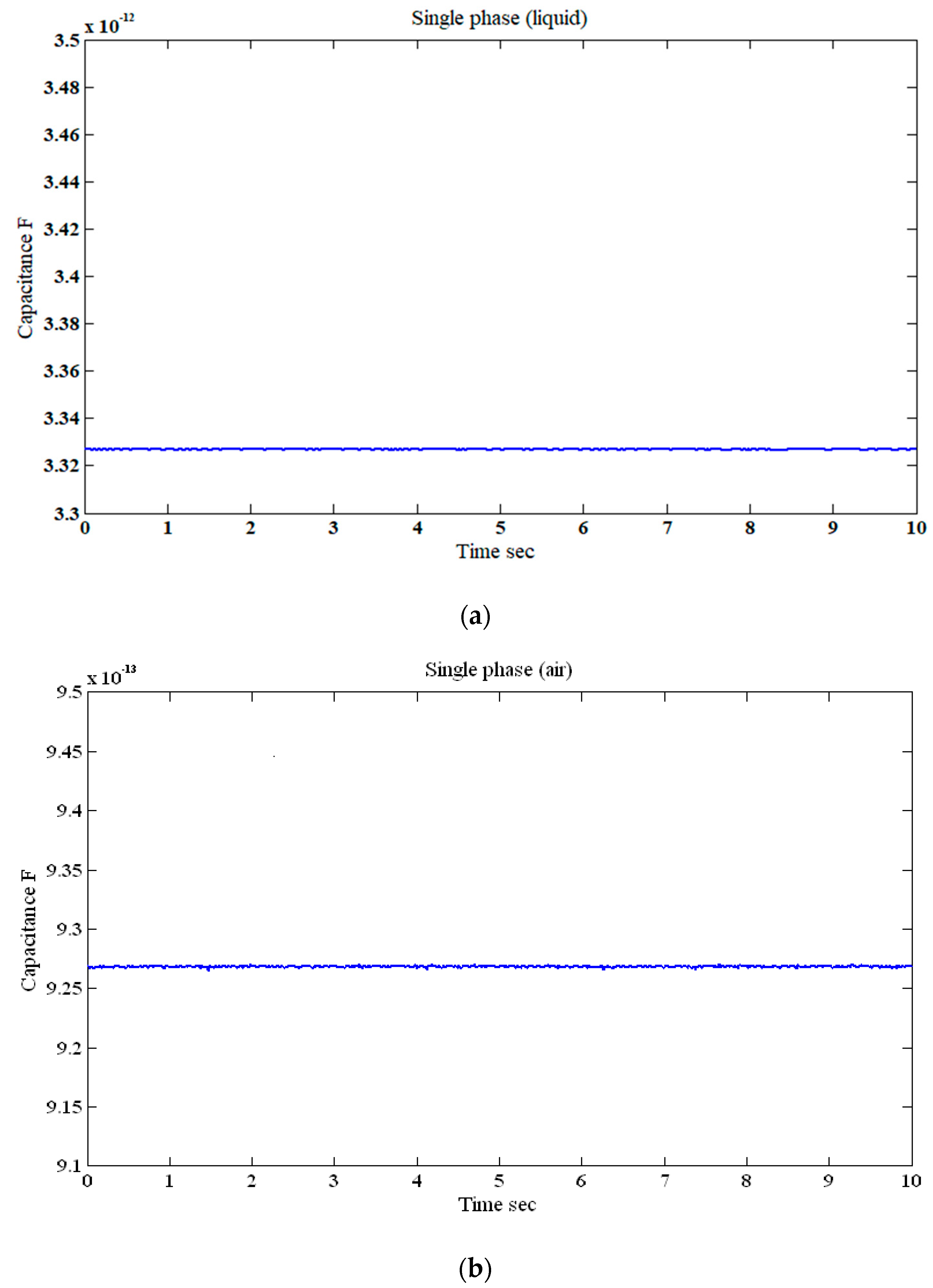
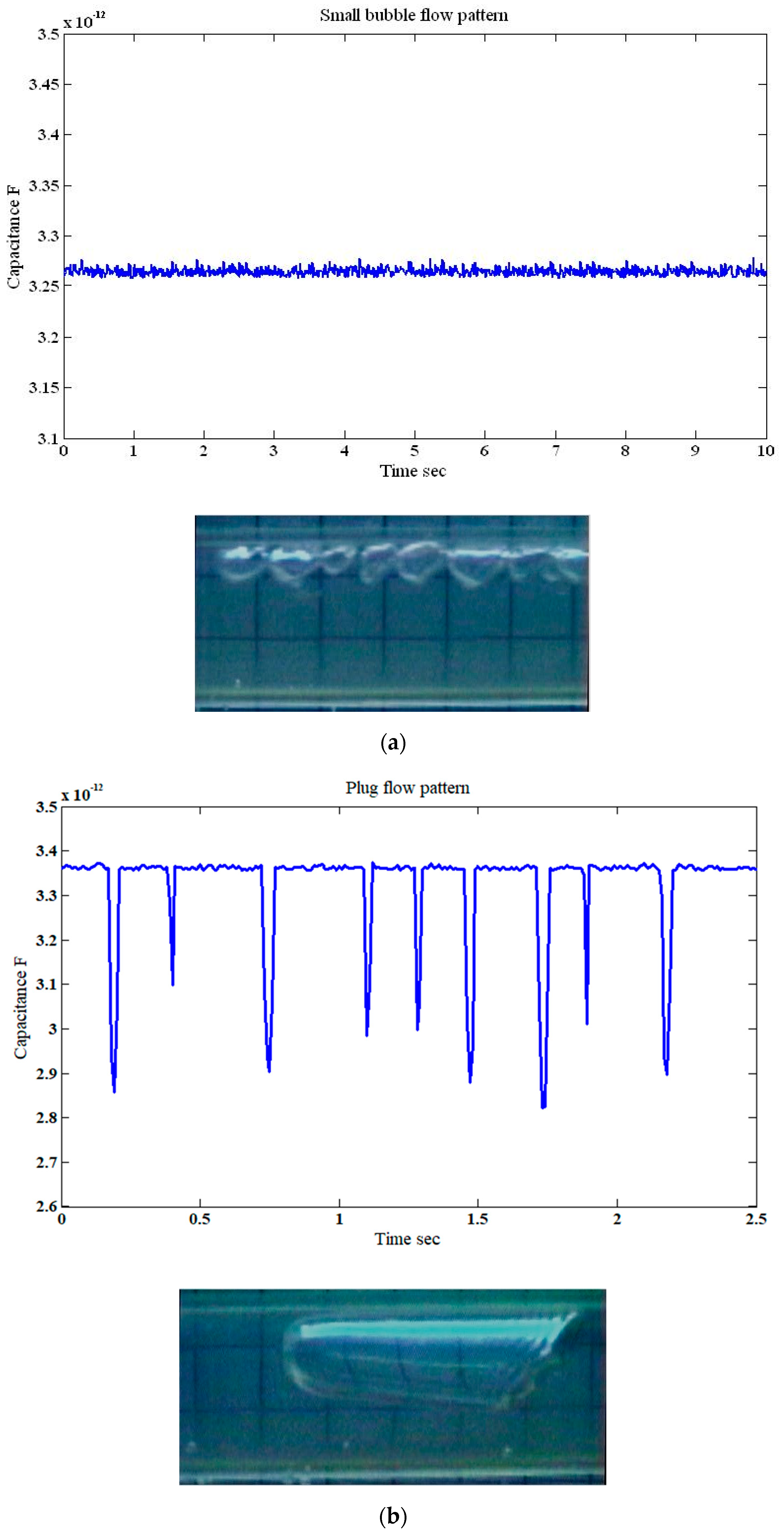
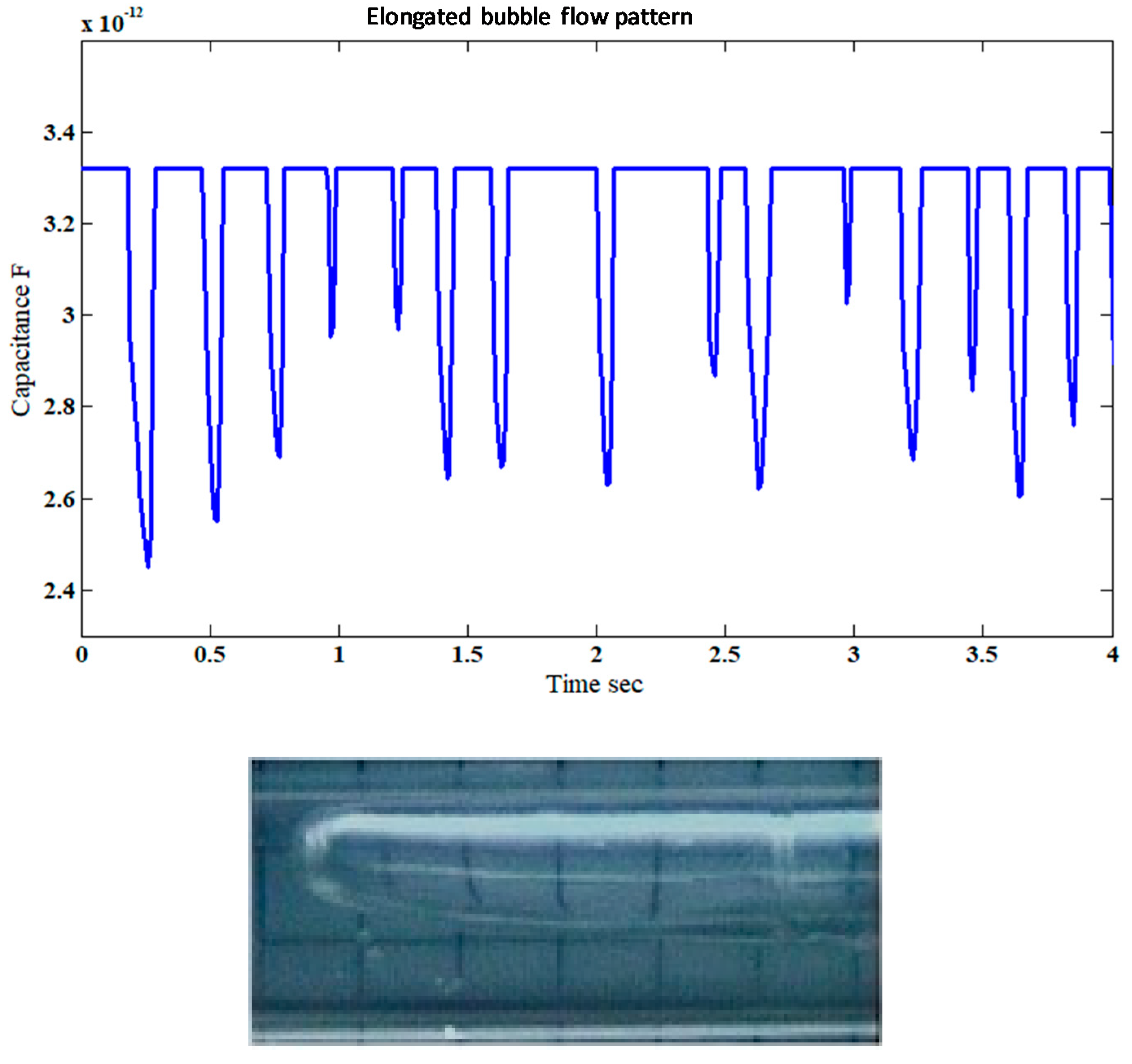
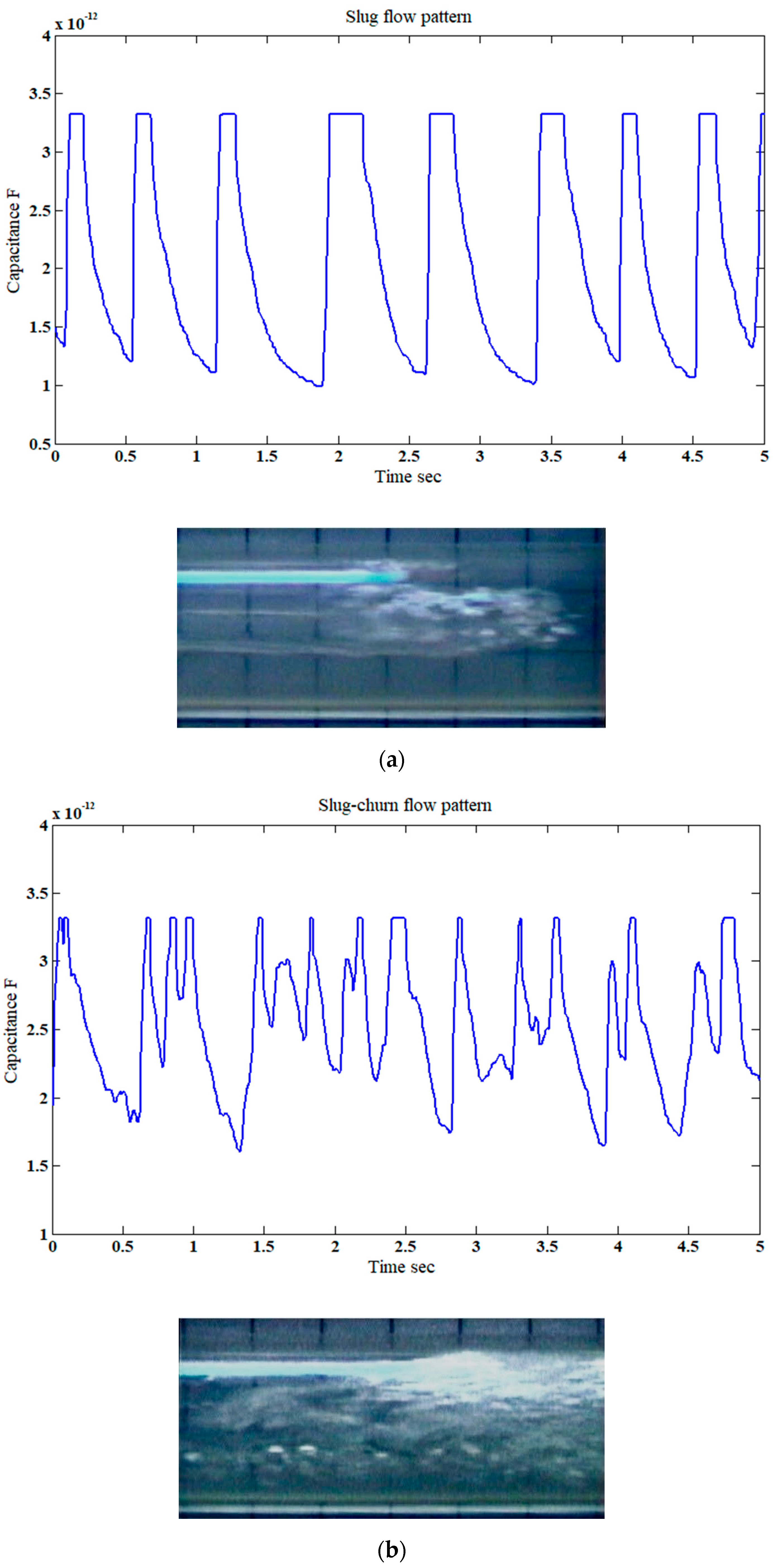
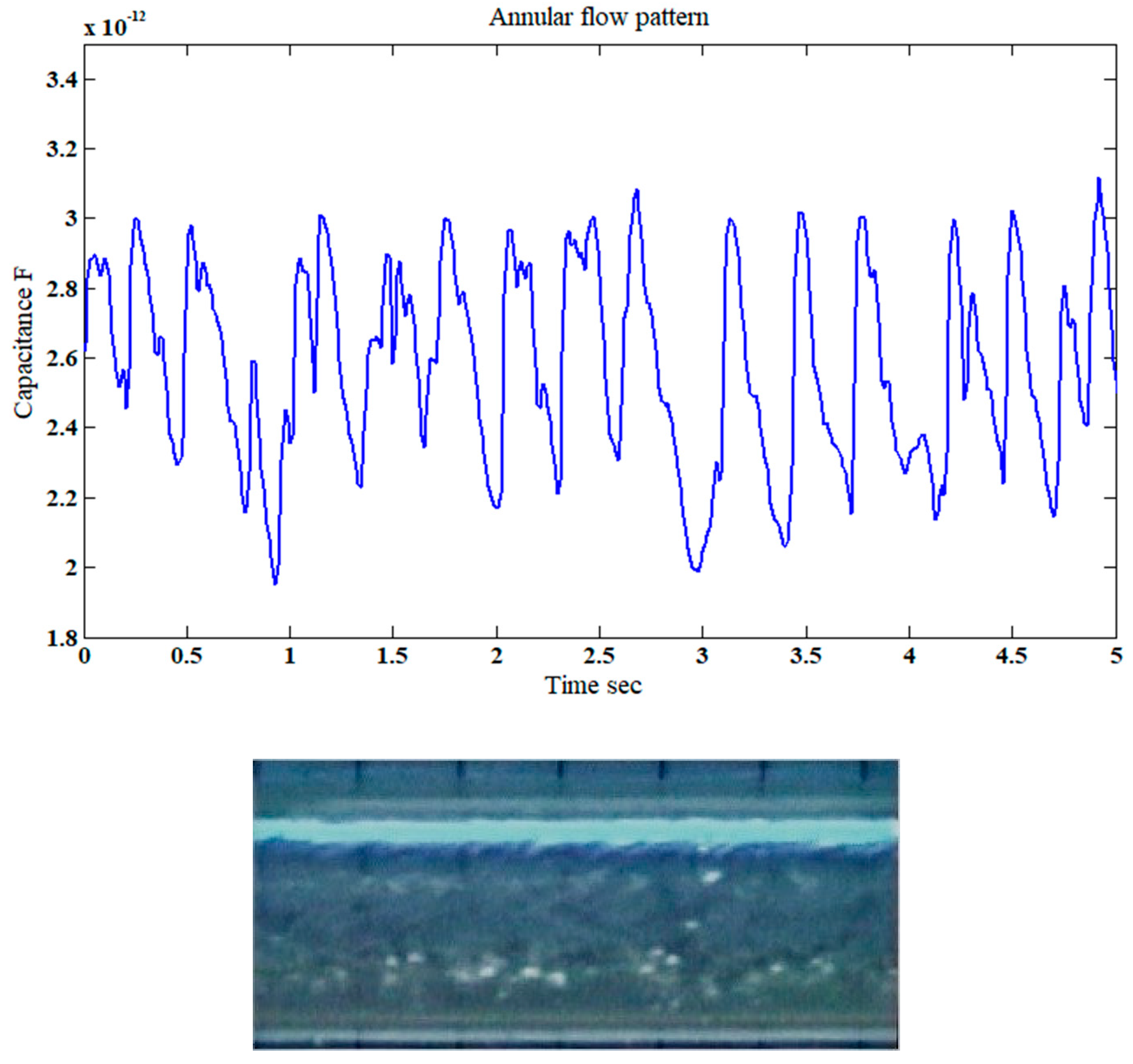
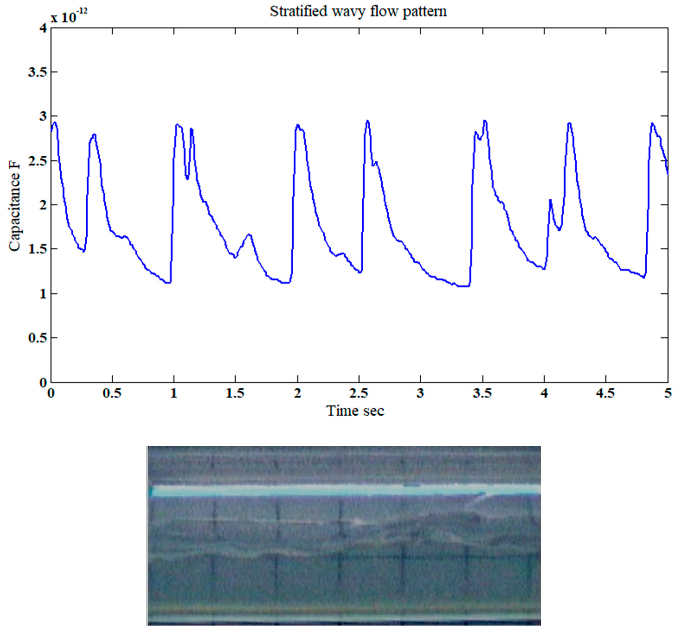
3.1. Capacitance Time-Dependent Analysis

Initial tests for single-phase (i.e., water or air) experiments were conducted to check the response of the capacitance sensor to each of the phases as a function of time. Firstly, a single-phase flow of only water was performed; the capacitance value over time was a smooth line of about 3.33 pF, demonstrating the liquid phase capacitance, as shown in Figure 7a. This capacitance value is the highest measured value recorded in the presented experimental work. Later, a single-phase flow of only air was passed through the rig; the capacitance value over time was a smooth line of about 0.926 pF, demonstrating the gas phase capacitance, as shown in Figure 7b. This time, the capacitance value is the lowest measured value recorded in the presented experimental work. The difference between both values (i.e., capacitance for only liquid and only gas) comes from their dielectric permittivity. This is because water has a higher dielectric permittivity than air. These values will be treated as reference points on which we confirm that there is no noise involved on the capacitance time-dependent values.
The measured capacitance values as a function of time were found to demonstrate the correct illustrative view of the flow patterns agreeing with their visual categorization and their typical well-defined characterization. Selected samples of the capacitance values as a function of time for different gas–liquid superficial velocities and inclinations are shown in Figure 8, Figure 9, Figure 10, Figure 11 and Figure 12 (representing the ideal flow patterns). Snapshots of the selected typical flow patterns are also shown, as cropped images.
The defined characteristic of small bubble flow pattern in a multiphase flow system is that the liquid phase occupies a greater volume fraction of the pipe (i.e., high liquid holdup, Figure 2), while the gas phase in the form of small bubbles at the top section of the pipe is characterized by low holdup or volume fraction. Therefore, as bubbles passed through the capacitance sensor, little fluctuation was observed. This was confirmed against liquid only system as shown in Figure 7a, where the capacitance value was a straight line demonstrating the capacitance of the liquid phase passing the capacitance sensor. The observed capacitance traces for small bubble flow in Figure 8a were almost similar to that of only liquid phase. Nevertheless, small capacitance fluctuations are measured indicating the presence of a second phase, which is the gas in the form of small bubbles. This is because the dielectric permittivity of the gas phase is different than that of the liquid phase.
As the superficial gas and liquid velocities are increased, the bubbles size in the pipe is increased. The small bubbles are merged together to form larger size bubbles, named plug flow pattern. As shown in Figure 8b, the liquid phase is indicted by high capacitance values, while the plug (i.e., the cap-bubbles), which is the gas phase, is indicated by low capacitance values. Therefore, as the cap-bubbles passed through the sensor, a successive fall in the capacitance values that occurred intermittently was observed. There was a quantity of small bubbles that did not have the sufficient momentum to coalesce and form a plug. These small bubbles manifest themselves as small fluctuations in the horizontal axis at the high range of capacitance trace.
A similar trend was observed for the elongated bubble flow pattern when compared with the plug flow pattern case. However, at this time, the size of the bubbles was even larger than that of the plug flow pattern and occupied slightly more than 50% of the diameter of the pipe. The minimum values of the capacitance fluctuated about different ranges between 2.4–3 pF. This is because of the irregularity in the shape of the elongated bubbles, as shown in Figure 9.
For the slug flow pattern, different zones of a series of gas and liquid phases crossing the capacitance sensor were observed. The fluctuations of this flow pattern pronounced themselves as a variation on the capacitance values, as shown in Figure 10a. It was similar for the slug-churn flow, which was generated as a result of additional development of slug flow regime. Here, the interchangeable nature between the gas and liquid phases caused the capacitance to fluctuate. However, the liquid in the slug became very frothy as a result of merging between the two phases as the superficial gas–liquid velocity ratio increased. Hence, the fluctuations were more intense with irregular profile when compared to the slug flow pattern, as shown in Figure 10b.
For the annular flow pattern, the gas phase occupied the core of the pipe, whereas the liquid phase formed an irregular thick film adjacent to the pipe wall which is at the pipe’s annulus. As such irregular waves continuously flowed around the pipe boundary wall, the created interface caused the capacitance values to fluctuate, as shown in Figure 11. In this flow regime, the minimum values of the capacitance traces almost double to about 2 pF when compared to slug and slug-churn flow patterns. This is due to the actual structure and continuous existing of the annular flow and its corresponding film distribution around the pipe, which as a result, influenced the electrical field distribution inside the pipe and its corresponding capacitance values. The stratified flow pattern has two distinguished phases with no intermixing between them. Those phases are a liquid phase passing along the bottom section of the pipe, a gas phase at the top section of the pipe, and a wavy interface existing just between the two phases (Figure 12).

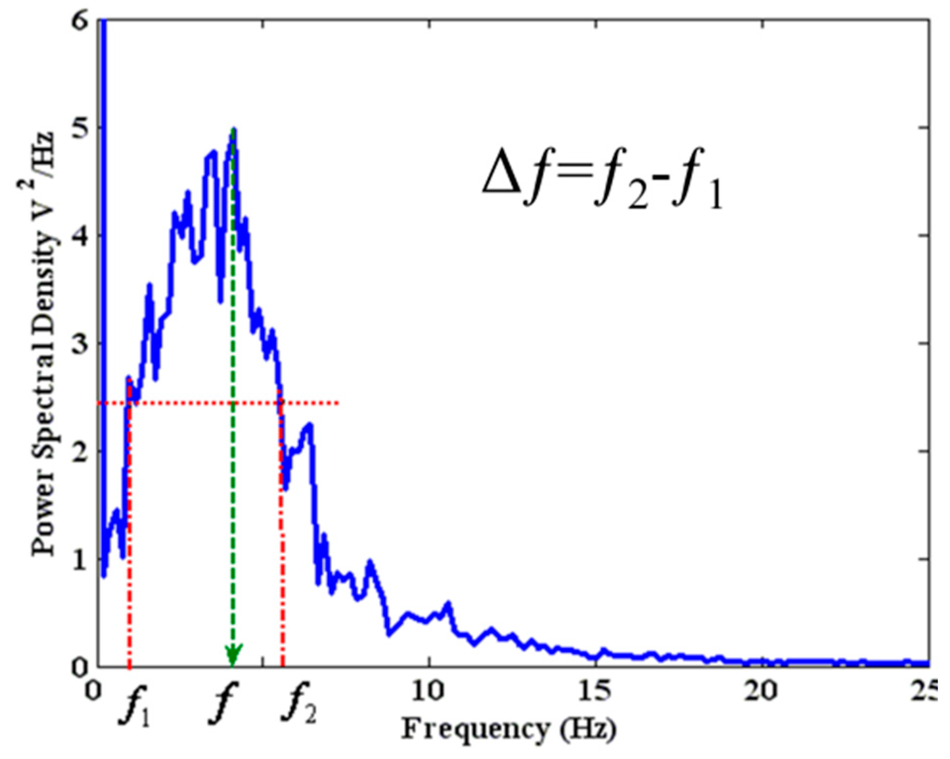
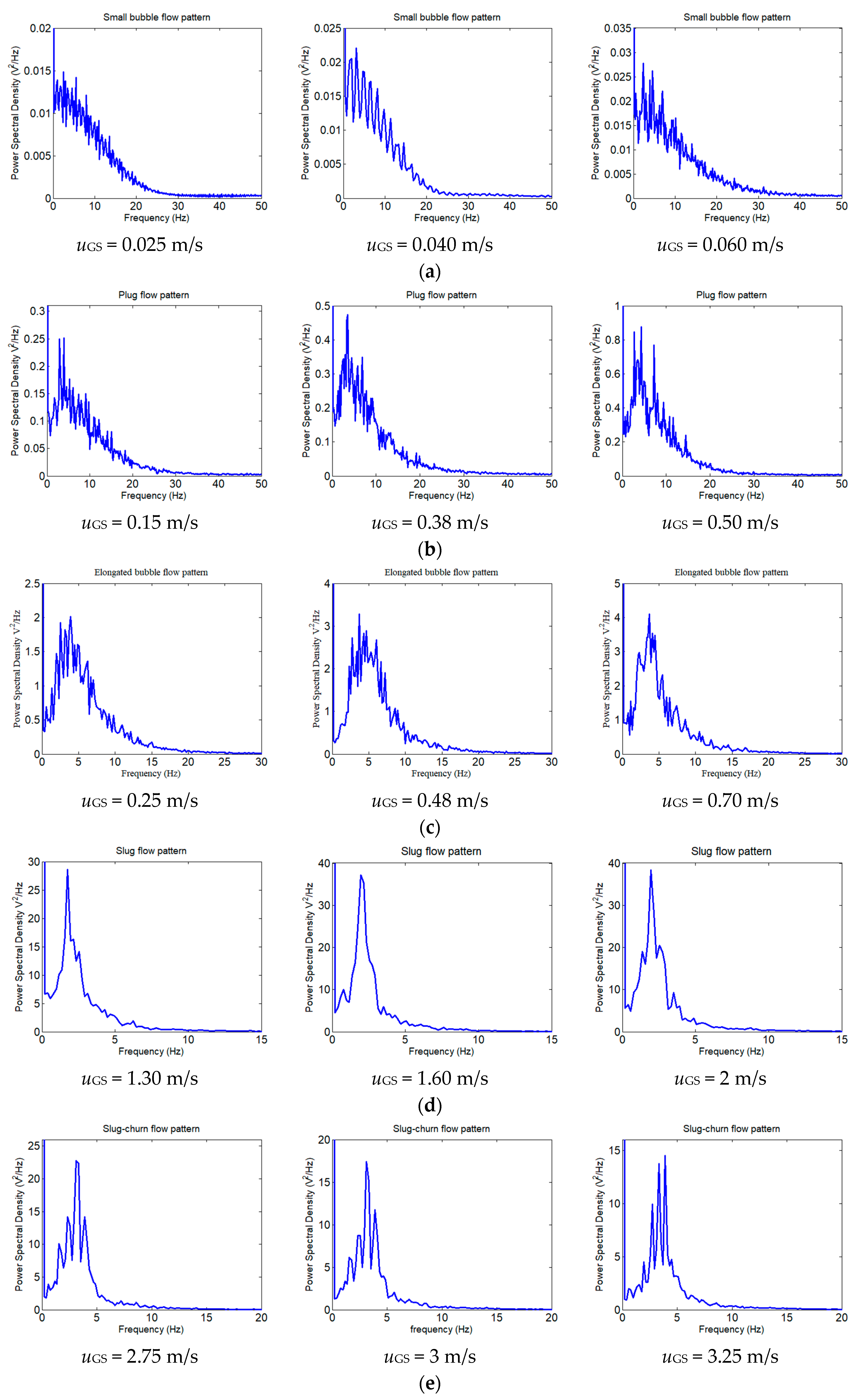
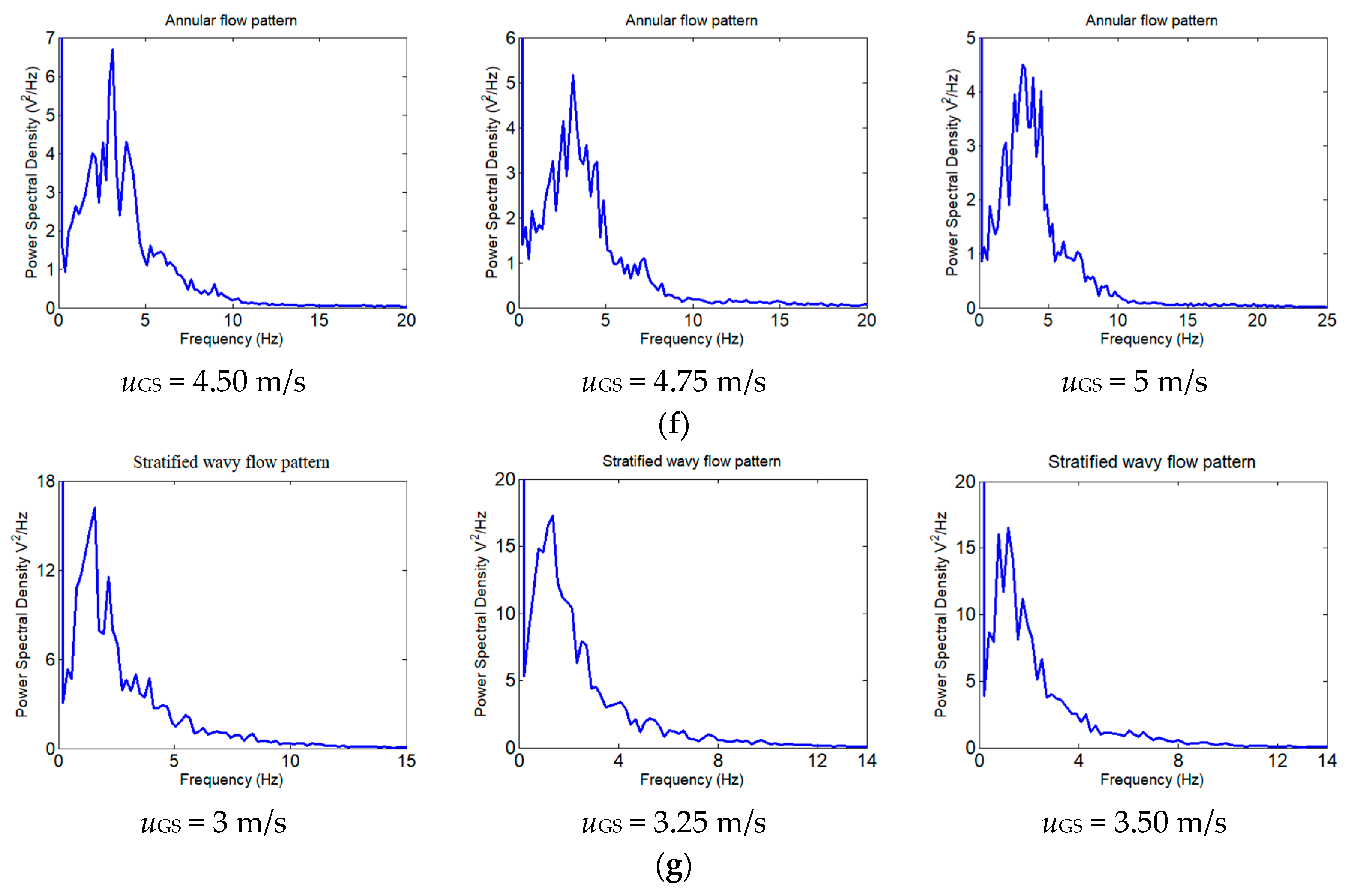
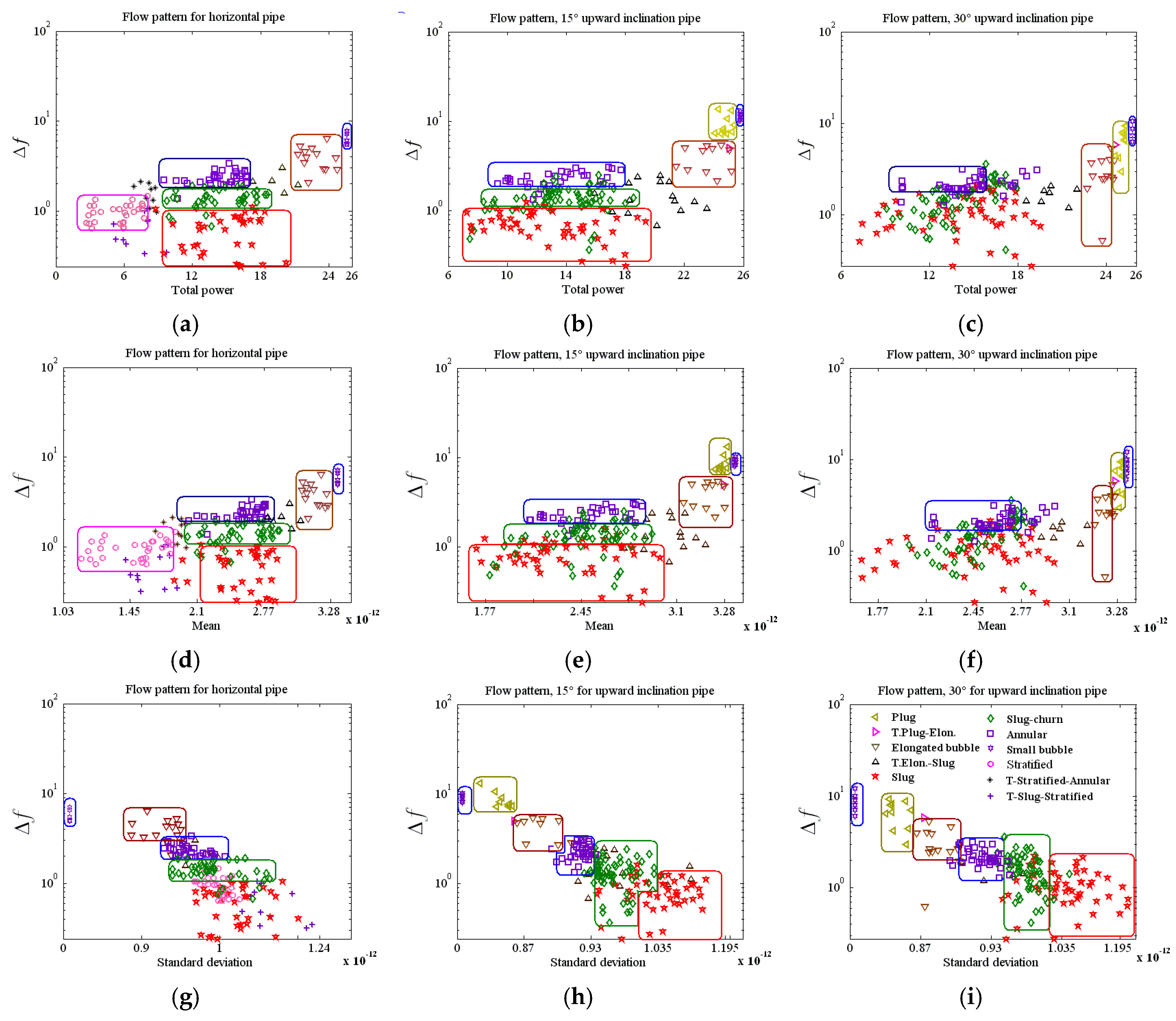
3.2. Frequency Analysis

The power spectral densities were computed using the voltage output of the capacitance sensor for all the typical flow patterns. Samples of the PSD spectrum for the intermittent flow patterns are shown in Figure 13a–d, and those for the chaotic flow patterns are shown in Figure 13e–g.
The PSD for the small bubble flow was characterized by the lowest amplitude (Figure 13a). This is probably because as small bubbles are passed through the capacitance, it induced small fluctuations in the capacitance and represented itself as a low PSD spectrum signal. As the gas–liquid superficial velocities increased, a plug flow pattern was developed. The PSD for the plug flow was characterized by many small spikes. Therefore, multiple dominant amplitudes of these spikes were found. This is because of the irregular structural/shape of the bubbles, and the presence of small bubbles which did not coalesce to form plugs. As shown in Figure 13b, these fluctuations in the PSD spectrum are actually the fluctuations in the liquid holdups, which manifested themselves as multiple dominant PSD frequencies [2]. In addition, as further increases in the gas and liquid superficial velocities are applied, the plug bubbles coalesced and formed elongated bubbles. The PSD of the elongated bubble flow had defining spikes which were characterized by higher amplitude values almost five times greater than that of the plug flow pattern. The spikes were also fewer in number when compared to plug flow pattern (Figure 13c).
As the gas–liquid superficial velocities were increased, the experimental conditions were now at a critical point between the intermittent regions and chaotic regions. The small and multiple spikes that characterized most of the intermittent flow regions and its PSD spectrums (shown in Figure 13a–c) have disappeared, as shown in Figure 13d for the slug flow, Figure 13e for the slug-churn, Figure 13f for the annular flow, and Figure 13g for the stratified wavy flow. For all the flow patterns that were developed, the PSD value for slug flow was characterized by the highest and sharpest spike. This is because the slug flow pattern is at the critical point between the intermittent and the chaotic flow. In addition, as the slug-churn flow was developed, it was found that it had several spikes or dominant frequencies, but the PSD amplitude values were decreased when compared with the slug flow. It is believed that such clear differences in the PSD amplitude values between the slug and slug-churn flow patterns resulted from the internal mechanism of the flow patterns. This is because the slug-churn flow pattern is a mixture of a frothy liquid and small bubbles.
The annular flow is characterized by a liquid film adjacent to the pipe wall and a gas phase in the core of the pipe. Due to the variation in the thickness of the liquid film, the PSD of the annular flow was characterized by several dominant amplitudes. With exception to small bubble, plug and elongated bubble flow patterns, the PSD amplitude for the annular flow was lower than the calculated PSDs for most of the flow patterns. As the liquid flow rate was increased, the amplitude of the PSD for the annular flow slightly increased. This is because the capacitance registered a slightly stronger value. In addition, greater PSD amplitude value than that of the annular flow was measured, as the gas–liquid superficial velocities increased, and the stratified flow pattern was reached. It was also observed that there is some similarity in the PSD shapes between the stratified flow and slug flow, and both flow patterns were characterized by sharp spikes. This is because the stratified flow was treated by the FFT as a slug flow.
It is very important to investigate the PSD analysis for a wide range of flow formations and patterns. Owing to the fact that the behavior and shape of the PSD amplitude are indications on the variation of the captured signals and its corresponding frequencies and their intensity, the value of Δƒ is largely influenced by the induced changes on the amplitude of the PSD for each developed flow pattern. The obtained values of Δƒ from the PSD data along with the statistical parameters defined in the previous section will be used in the next discussion section to propose a new method to distinguish and discriminate between each flow pattern.

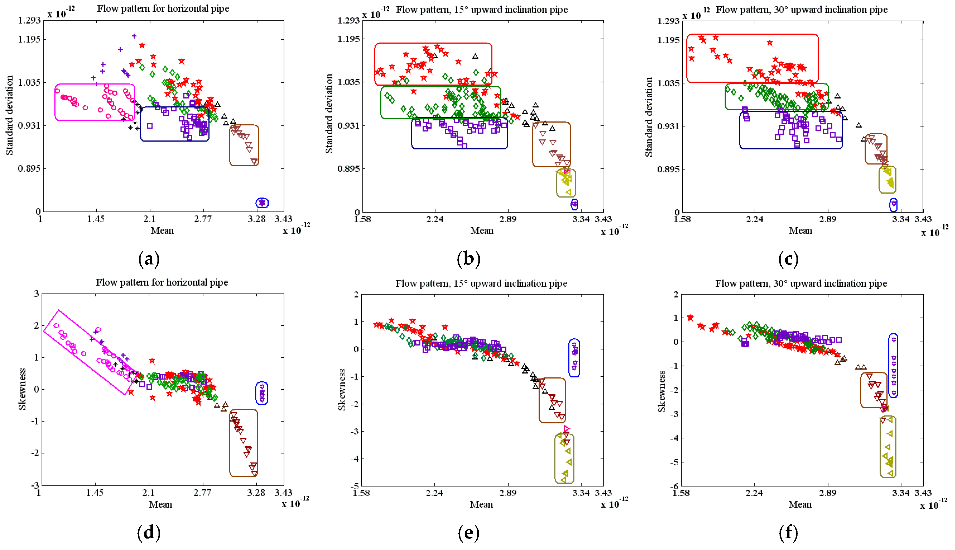
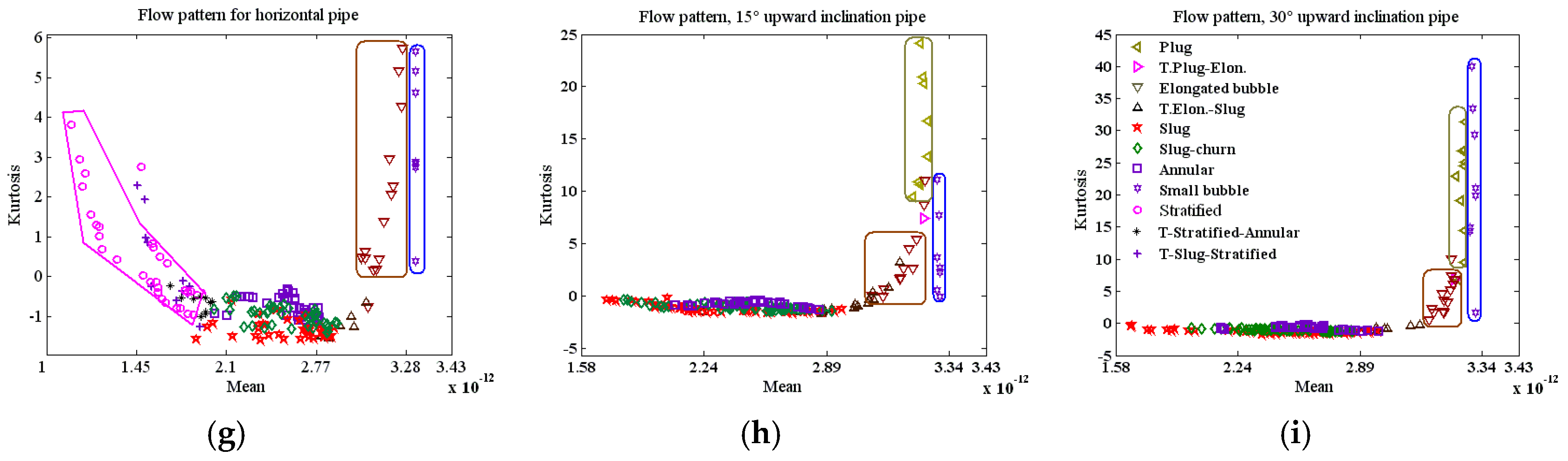
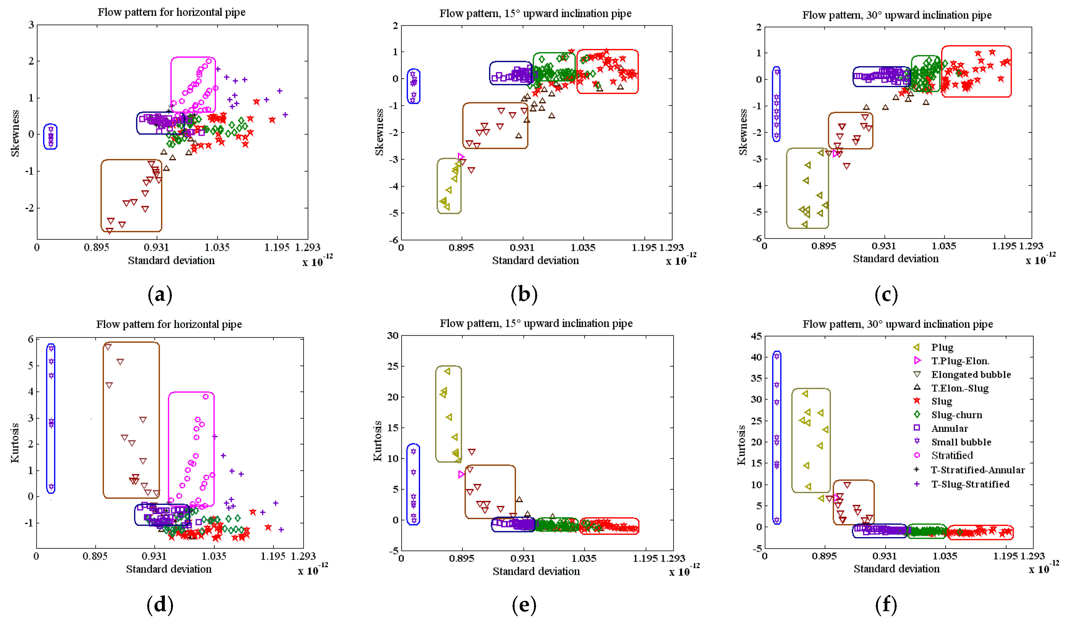
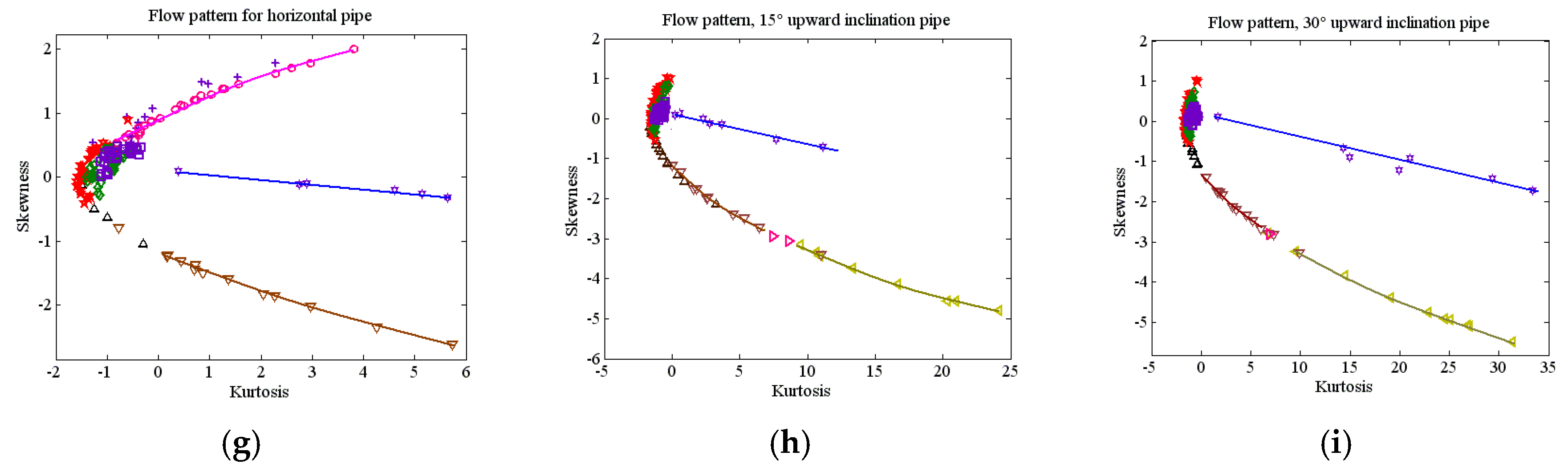
3.3. Statistical Analysis

The flow patterns investigated in this work are shown in the form of a flow pattern maps as a function of different gas–liquid superficial velocities, where each developed pattern was distinguished by different color and symbol (Figure 2). A statistical analysis method on the fluctuations of the capacitance sensor signals was conducted, where these fluctuations are believed to be strictly associated to the induced flow patterns. Thus, a new approach is proposed for identifying the developed flow patterns in a multiphase gas–liquid flow system with a circular pipe. This technique was applied on all the experimental cases and for each of the selected pipe angles: 0°, 15° and 30°. The approach is based on finding a relative correlation and interrelationship between the statistical and power spectrum parameters. These parameters were plotted against each other, so the standard deviation ( σ ¯ , 2nd parameter), the skewness ( γ 1 , 3rd parameter) and the kurtosis ( γ 2 , 4th parameter) were plotted against the mean (m, 1st parameter), γ 1 and γ 2 were also plotted against σ ¯ , and finally γ 1 was plotted against γ 2 .
For each examined angle, the σ ¯ values were plotted against the m values obtained from the sensor output, as shown in Figure 14a–c. Different fields correspond to different flow patterns and their various mechanisms were created from these plots. The dispersion of the data points in different fields may be the artefact of the following factors: (a) the various sizes and numbers of bubbles, (b) the intermittent nature of liquid slugs, (c) the variations of slug-churn, (d) the inconsistencies in the liquid phase thickness in the annular flow, and (e) the distinct mechanism of the waves in the stratified flow pattern, whereas all these factors are influenced by the changes in the gas–liquid superficial velocities. Figure 14a–c shows a distinct individual field for each flow pattern, however, the slug flow and the slug-churn flow in the horizontal orientation were overlapped. The reason behind this can be attributed to that just before the development of the slug or slug-churn flow at an angle of zero degree, the liquid phase filled nearly 25% of the diameter of the test pipe. Thus, almost the same values of σ ¯ are measured, and slight differences in amplitude between the two flow patterns were observed. As a result, the two sets of data points have a tendency to overlap with each other.
On the other hand, in the inclined cases just before the flow passed the capacitor at the measurement point, owing to the gravity effect, the pipe was almost unoccupied by any phase. Consequently, as the liquid slug passed through the capacitance sensor, large values of PSD amplitude were measured. However, a PSD value that was characterized by a lower amplitude when a chaotic slug-churn flow was passing the capacitance sensor is observed. This is the artefact of the intermittent nature of the signal, which led to a considerable variation in the amplitude values between the slug and slug-churn flow patterns. At 15° and at 30° inclinations, even though the m values between the slug and slug-churn flow patterns were almost similar, however, there was some variation in the values of σ ¯ . It is believed that this is because σ ¯ is largely sensitive to the variation in the length of the small intermittent characteristics of the capacitance output signal. Thus, different values of σ ¯ were measured between the slug and slug-churn flow patterns. It is also important to note that all flow patterns, including the stratified flow pattern, were developed in the horizontal case (except the plug flow), while for the inclined cases, no stratified flow pattern was developed. These observations agree well with the current reported results in the literature [10].
For the small bubble flow shown in Figure 14a–c, the variation in the values of m and σ ¯ were very insignificant. The values of m were about 3.28 pF and σ ¯ values varied closely around zero. As the liquid phase occupied most of the pipe which had a larger permittivity, the sensor capacitance value was large, whereas the air bubbles positioned at the upper section of the pipe had minor effect on the sensor value. Thus, only a slight fall in the capacitance value from a single liquid-phase was observed. The drop was from 3.34 pF for liquid only phase to 3.28 pF for the small bubbles pattern. For the plug pattern, the values of m and σ ¯ were very small. The values were between 3.25 and 3.27 pF and 0.495 and 0.895 pF for m and σ ¯ , respectively. This can be explained by the mechanism of the plug flow. In this case, the test pipe was fully occupied by liquid, which resulted in a large m value. When the elongated bubble flow pattern appeared interchangeably, a small fluctuation in the value of m, and therefore, in the value of σ ¯ was observed. The values of m and σ ¯ varied according to the depth of the elongated bubble, where both values were greater than that of the plug flow, owing to the size of the bubbles. As a result, m and σ ¯ values were between 3 and 3.2 pF and 0.895 and 0.93 pF, respectively. For all examined inclinations, the values of m and σ ¯ were almost equal. However, the small differences in the values of σ ¯ can be attributed to the variation in the thickness of the liquid phase. Additionally, Figure 14a–c shows the transitions and progressions between various flow patterns: (1) from stratified to annular flow, (2) from plug to elongated bubble, (3) from elongated bubble to slug, and (4) from slug to stratified.
For each examined angle, the γ 1 values were plotted against the m values obtained from the sensor output, as shown in Figure 14d–f. It is very clear that these figures cannot be used to distinguish between any flow pattern or to be used as a flow pattern identifier. This is because the figures showed a clearly defined field for only four flow patterns (i.e., stratified, small bubble, plug and elongated bubble). However, significant overlaps were observed between the slug, slug-churn and annular flow patterns for all inclinations. It also had nearly the same range of γ 1 values, that were between 1 and −1. Moreover, it was also observed that the bubbles size influenced the value of γ 1 . The plug flow had smaller bubble size than that of the elongated bubble flow. Therefore, from Figure 14d–f it can be seen that the values of γ 1 for the plug and elongated bubble flow patterns were located at the negative side of the figure, where the plug and elongated bubble flow patterns were characterized by large and small negative values, respectively. The values of γ 1 for the small bubble flow fall within the boundary of zero, though several points were observed to cluster toward the negative side of the figure. Again, for each examined angle, the γ 2 values were plotted against the m values obtained from the sensor output, as shown in Figure 14g–i. Similar behavior was observed between Figure 14d–f,g–i. The following set of flow patterns were observed in both figures: (1) for the horizontal case, only the fields for stratified, small bubble, and elongated bubble flow patterns can be identified, and (2) for the examined inclinations, only the fields for small bubble, plug and elongated bubble flow patterns can be identified. Strong overlapping and clustering are shown in the figures between the slug, slug-churn and annular flow patterns, where their values of γ 2 were slightly less than zero. Consequently, even the utilization of two sets of these figures together will not help in identifying slug, slug-churn or annular flow.
Later, for all the examined inclinations, the values of γ 1 were plotted against the values of σ ¯ , as shown in Figure 15a–c. As formerly shown in the plots of σ ¯ against m (Figure 14a–c), a distinct field for each flow pattern was observed. An exception was also observed for the slug and slug-churn flow patterns in the horizontal case, which were clustering without any distinct fields. For all the examined inclinations for slug, slug-churn and annular flow patterns, the values of γ 1 were between 1 and −1. Additionally, in plug flow, the values of γ 1 were limited between −3 > γ 1 > −6 for 15° and 30° inclinations. It is important to point out that all the developed flow patterns had relatively similar positions and range of values regardless of their angles. Lastly, similar to Figure 14a–c, the transitions and progressions between various flow patterns were located among their own respective fields.
Similarly, for all the examined orientations, the values of γ 2 were plotted against the values of σ ¯ , as shown in Figure 15d–f. The resulted figures showed that all the flow patterns could be recognized by their distinctive fields. However, once more, an exception was also observed for the slug and slug-churn flow patterns in the horizontal case which were clustering without any distinct fields for similar reasons that were discussed before. From these analyses, it is now noticeable that the value of σ ¯ shows a significant role in the discrimination between different flow patterns in multiphase flow. A clear and comprehensively distinguished field appeared for most of the developed flow patterns when σ ¯ was used as a factor in the figures more than the other parameters. This is because the value of σ ¯ represents the amplitude fluctuation of the output signal, which is triggered by the flow of the used phases through the capacitance sensor. As mentioned earlier, the size of the air bubbles caused the difference observed between the plug and elongated bubble flow. This difference is based on (a) the variation of the recurring rise and fall in the liquid holdup, and (b) the fluctuations of the capacitance output signals. In brief, the variation in the bubble size influenced the value of σ ¯ . In the slug and slug-churn flows, σ ¯ points to the average amplitude of the fluctuating output of the capacitance sensor. Therefore, the values of σ ¯ were larger owing to the fluctuations that were caused by the liquid phase flow interchanging with the gas phase flow, which were recurrently passing the capacitance sensor. In the annular flow, the value of σ ¯ exhibits the variations of the thickness of the liquid film inside the pipe. Finally, in the stratified flow pattern, the values of σ ¯ were influenced by the distinct mechanism of the liquid waves and its mean height, as shown in Figure 12.
The importance of the standard deviation values ( σ ¯ ) as a factor that can be used to differentiate between all gas–liquid flow patterns is evident in the last set of graphs shown in Figure 15g–i. As can be seen in these graphs, when γ 1 was plotted versus γ 2 , only a small number of flow patterns were identified. These flow patterns are the first three intermittent patterns, namely the small bubble, plug and the elongated bubble, in addition to one flow pattern at the high flow rate, which is the stratified flow pattern. Meanwhile, the values of γ 1 and γ 2 for the slug, slug-churn and annular flow patterns were overlapping almost about the zero value.
In addition, for all examined inclinations, Figure 16a–c shows distinct fields as a result of plotting the values of Δƒ (that were obtained from the PSD analysis) against the total power of the output signal. It can be seen that all the developed flow patterns had their own discrete field. However, due to the large similarity in the internal mechanism between the slug and slug-churn flow patterns, the FFT analysis regarded the slug as a slug-churn and the values of Δƒ were comparable [69]. Therefore, an overlapping behavior was observed between the slug and slug-churn at the angle of 30°. It is also believed that this overlapping feature is the artefact of the aerated liquid phase at 30°. It is worth noting that from Figure 16a–c, the value of Δƒ increased as the inclination increased, principally for slug flow pattern at 30°. This is again due to the change in the shape of the PSD and the decrease measured in its amplitude values, where both correspond to the pipe hydrodynamic status. For each flow pattern, the total power value ranges were different. Moreover, it was shown earlier in Figure 14 and Figure 15 that the data points for slug and slug-churn flow pattern at 0° inclinations were overlapping to the degree that they cannot be differentiated from each other (Figure 14a–c and Figure 15a–c). It is therefore notable that in Figure 16a–c, the relation between Δf and total power succeeded in splitting them into distinct fields. Additionally, similar to Figure 14 and Figure 15, there were some observed transitions and progressions between various flow patterns.
As can be seen, Figure 16d–f were almost identical to Figure 16a–c. Since the two sets of figures are indistinguishable, using them together will not assist to differentiate between slug and slug-churn at 30°. It was for that reason we decided to draw the values of Δƒ versus that of the σ ¯ . This is because the standard deviation is highly associated to the power of the signal and its fluctuation. Figure 16g–i showed very clear identification for all flow patterns at each inclination, but overlapping data with no distinct fields were observed for the slug and stratified flow patterns in the horizontal cases. Nevertheless, these distinct fields were observed evidently in both Figure 16a,d (i.e., for the horizontal case). Therefore, by combining either of these figures, that is Figure 16a–c or Figure 16d–f with Figure 16g–i, allowed the identification of all the developed flow patterns. It can be concluded that by associating two sets of these graphs, all the generated (gas–liquid) flow patterns in a multiphase flow system can be distinguished. The first set is associating Δƒ with any variable of the statistical factors or the total power of the signal, and the second set is associating σ ¯ against any statistical factors or Δƒ.
The last group of figures was drawing the ratio of the frequency (i.e., Δƒ/ƒ) against the Reynolds number (Re) of the gas–liquid mixture for all the examined angles, as shown in Figure 17a–c. From the first instance, it is very clear that this approach is not capable of identifying all flow patterns. In addition, these figures demonstrated that the examined angles influenced the locality of the flow patterns and their transitions from one flow pattern into the other. As evident from this set of figures, there was substantial overlying of data associated with many of the developed flow patterns (for instance: (1) the stratified flow data overlapped with the slug-churn flow data in the horizontal cases, and (2) the progressions from slug flow to stratified flow also overlapped with the elongated bubble flow data). Consequently, the uncertainty of this dimensionless factor (i.e., Re) to classify different flow patterns is high. Since the techniques that were applied in Figure 17 were similar to that of Figure 14, Figure 15 and Figure 16, the only noteworthy change being that the values of Re were not calculated from the output of the capacitance sensor. The capability to distinguish between different gas–liquid flow patterns appears to be superior when using (a) the four statistical (m, σ ¯ , γ 1 and γ 2 ), and (b) the power spectrum parameters (Δƒ and the total power of the signal). This is because all these six parameters were actually obtained from the output of the capacitance sensor.
A summary and comparison of the statistical and power spectrum parameters which were used to identify different flow patterns for multiphase gas–liquid flow at different inclinations are shown in Table 1. The above discussion showed that this recommended approach of mapping these factors can consistently differentiate between all flow patterns. The investigation conducted on the utilized frequency and statistical factors showed that the standard deviation ( σ ¯ ), the width of the characteristic frequency peaks (Δƒ), and the mean (m) are the most important factors. When these factors were associated together in one graph, nearly all flow patterns were able to be detected, except a couple of flow patterns that were not identified as shown in Table 1. However, combining two sets of these graphs, for example, (a) σ ¯ vs. Δƒ with Δƒ vs. m (or Δƒ vs. total power), (b) Δƒ vs. total power with γ 1 vs. σ ¯ (or γ 2 vs. σ ¯ ), and (c) σ ¯ vs. m with Δƒ vs. m (or Δƒ vs. total power), allowed all flow patterns to be identified clearly at all inclinations.
It is worth noting that the main disadvantages of this simple two electrodes capacitance design can be concluded in the following remarks:
  • It cannot construct tomography images in comparison with sensors that consist of eight or more electrodes.
  • It suffers from lower resolution when compared to sensors with more than two electrodes (especially for large diameter pipes).
  • It has high uncertainty in void fraction measurements (especially for post-intermittent flow regimes) when compared with sensors that have more than two electrodes.
However, the above reported experimental results proved that such a simple and inexpensive configuration can reliably be utilized in addition to the proposed approach to successfully distinguish between different generated flow patterns in a multiphase gas–liquid flow system.

4. Conclusions

A new technique is proposed in this study to distinguish between different flow patterns in a multiphase flow system. It was executed by using specially designed electrical capacitance sensor through systematic and extensive experimental program. The capacitance measurement sensor consisted of two electrodes with a concave shape which was fixed on the experimental setup and a suitable data acquisition method was established. The designed sensor was utilized for the detection of different flow patterns with the aid of a detailed analysis of the photographic data obtained from the high-speed camera. The time-dependent data of the output signal were collected from a multiphase air–water flow system with a circular pipe for different inclinations (horizontal, upward 15° and upward 30°) and large combinations of superficial gas and liquid velocities.
This technique depends on analyzing the interrelationship between the frequency and the statistical parameters to identify each generated flow pattern. For that reason, a systematic evaluation of the effectiveness of quantity of these parameters in identifying different gas–liquid flow patterns at different inclinations was conducted. Firstly, each of the four statistical parameters (m, σ ¯ , γ 1 and γ 2 ) obtained from the capacitance sensor signals were plotted against each other. Then, some of the power spectrum parameters were considered, namely the width of the characteristic frequency peaks (Δƒ), the total power of the capacitance signal and the frequency ratio (Δƒ/ƒ). Moreover, the last parameter that was evaluated was the Reynolds number of the mixture. The results showed that some parameters found to be highly important than the others such as m, σ ¯ and Δƒ. The identification of all flow patterns generated inside a circular pipe of a multiphase gas–liquid flow system at different angles can be realized by combining the following sets of statistical graphs: (a) σ ¯ vs. Δƒ with Δƒ vs. m (or Δƒ vs. total power), (b) Δƒ vs. total power with γ 1 vs. σ ¯ (or γ 2 vs. σ ¯ ), and (c) σ ¯ vs. m with Δƒ vs. m (or Δƒ vs. total power). It is therefore believed that the approach reported in this paper successfully identified, distinguished and characterized all the ideal flow patterns generated in a gas–liquid flow system. The positive results obtained from this approach may potentially have valuable applications in related academic and industrial research.

Author Contributions

Conceptualization, F.M.A.-A. and A.J.J.; formal analysis, F.M.A.-A. and A.J.J.; funding acquisition, F.M.A.-A.; investigation, F.M.A.-A. and J.K.; methodology, F.M.A.-A., A.J.J. and J.K.; validation, F.M.A.-A.; visualization, F.M.A.-A.; writing—original draft, F.M.A.-A., Y.A.A., Z.A., A.J.J. and J.K.; writing—review and editing, F.M.A.-A., Y.A.A. and Z.A.; Authors contributed equally in writing and preparing this work, F.M.A.-A., Y.A.A. All authors have read and agreed to the published version of the manuscript.

Funding

This work was completely funded by King Abdulaziz City for Science and Technology (KACST).

Acknowledgments

The first author would like to express his utmost gratitude to the King Abdulaziz City for Science and Technology, Petroleum and Gas Research Institute, Saudi Arabia, Riyadh (www.kacst.edu.sa), who supported him financially throughout this study. The author Yusif A. Alghamdi extends his gratitude to the Deputy of Research and Innovation DRI-MOE at the Kingdom of Saudi Arabia for the Postdoctoral Fellowship Program (PFP) and also recognizes the support provided by the Deanship of Scientific Research at King Saud University (DSR-KSU).

Conflicts of Interest

The authors declare no conflict of interest. The funders had no role in the design of the study; in the collection, analyses, or interpretation of data; in the writing of the manuscript, or in the decision to publish the results.

Nomenclature

Latin Symbols
CCapacitance (F)
CGGas capacitance (F)
CLLiquid capacitance (F)
C(statistical variable)Capacitance of the sensor value (F)
mMean value (F)
dinInner pipe diameter (mm)
doutOuter pipe diameter (mm)
fFrequency of the highest power spectrum (Hz)
ΔƒWidth of the characteristic frequency peaks (Hz)
NNumber of data points sampled
uGSSuperficial gas velocity (m/s)
uLSSuperficial liquid velocity (m/s)
utTranslational velocity (m/s)
Greek Symbols
ε 0 Permittivity of free space (F/m)
σ ¯ Standard deviation (F)
γ 1 Skewness
γ 2 Kurtosis
βInclination angle
Abbreviations
FFTFast Fourier Transform
PSDPower spectral density

References

  1. Soo, S.L. Dynamics of Multiphase Flow Systems. Ind. Eng. Chem. Fundam. 1965, 4, 426–433. [Google Scholar] [CrossRef]
  2. Alghamdi, A.Y.; Peng, Z.; Luo, C.; Almutairi, Z.; Moghtaderi, B.; Doroodchi, E. Systematic Study of Pressure Fluctuation in the Riser of a Dual Inter-Connected Circulating Fluidized Bed: Using Single and Binary Particle Species. Processes 2019, 7, 890. [Google Scholar] [CrossRef] [Green Version]
  3. Hua, L.; Lu, L.; Yang, N. Effects of liquid property on onset velocity of circulating fluidization in liquid-solid systems: A CFD-DEM simulation. Powder Technol. 2020, 364, 622–634. [Google Scholar] [CrossRef]
  4. Ekberg, N.P.; Ghiaasiaan, S.M.; Abdel-Khalik, S.I.; Yoda, M.; Jeter, S.M. Gas-liquid two-phase flow in narrow horizontal annuli. Nucl. Eng. Des. 1999, 192, 59–80. [Google Scholar] [CrossRef]
  5. Furukawa, T.; Fukano, T. Effects of liquid viscosity on flow pattern in vertical upward gas-liquid two phase flow. Int. J. Multiph. Flow 2001, 27, 1109–1126. [Google Scholar] [CrossRef]
  6. Van Hout, R.; Shemer, L.; Barnea, D. Evolution of hydrodynamic and statistical parameters of gas-liquid slug flow along inclined pipes. Chem. Eng. Sci. 2003, 58, 115–133. [Google Scholar] [CrossRef] [Green Version]
  7. Barnea, D. Transition from annular flow and from dispersed bubble flow-unified models for the whole range of pipe inclinations. Int. J. Multiph. Flow 1986, 12, 733–744. [Google Scholar] [CrossRef]
  8. Barnea, D.; Taitel, Y. Flow pattern in transition in two-phase gas liquid flows. Encycl. Fluid Mech. 1986, 3, 404–469. [Google Scholar]
  9. Al-Alweet, F. The Development of Capacitance Measurement Techniques and Data Processing Methods for the Characterisation of Two-Phase Flow Phenomena in Horizontal and Inclined Pipelines; The University of Manchester: Manchester, UK, 2008. [Google Scholar]
  10. Almutairi, Z.; Al-Alweet, F.M.; Alghamdi, Y.A.; Almisned, O.A.; Alothman, O.Y. Investigating the Characteristics of Two-Phase Flow Using Electrical Capacitance Tomography (ECT) for Three Pipe Orientations. Processes 2020, 8, 51. [Google Scholar] [CrossRef] [Green Version]
  11. Adewumi, M.A.; Bukacek, R.F. Two-phase pressure drop in horizontal pipelines. J. Pipelines 1985, 5, 1–14. [Google Scholar]
  12. Barnea, D.; Brauner, N. Hold-up of liquid in two phase intermittent flow. Int. J. Multiph. Flow 1985, 11, 43–49. [Google Scholar] [CrossRef]
  13. Ito, K.; Inoue, M.; Ozawa, M.; Shoji, M. A Simplified Model of Gas-Liquid Two-Phase Flow Pattern Transition. Heat Transf. Asian Res. 2004, 33, 445–461. [Google Scholar] [CrossRef]
  14. Bennett, D.; Woods, Z.F. Frequency and development of slugs in a horizontal pipe at large liquid flows. Int. J. Multiph. Flow 2006, 32, 902–925. [Google Scholar]
  15. Pongsiri, S.; Somchai, W. Tow-phase flow pattern maps for vertical upward gas-liquid flow in mini-gap channels. Int. J. Multiph. Flow 2004, 30, 225–236. [Google Scholar]
  16. Abouelwafa, S.M.; Kendall, E.J. The use of capacitance sensors for phase percentage determination in multiphase pipelines. IEEE Trans. Instrum. Meas. 1980, 28, 24–27. [Google Scholar] [CrossRef]
  17. Bangliang, S.; Zhang, Y.; Peng, L.; Yao, D.; Zhang, B. The use of simultaneous iterative reconstruction technique for electronic capacitance tomography. Chem. Eng. J. 2000, 77, 37–41. [Google Scholar] [CrossRef]
  18. Dyakowski, T.; Edwards, R.B.; Xie, C.G.; Williams, R.A. Application of capacitance tomography to gas-solid flows. Chem. Eng. Sci. 1997, 52, 2099–2110. [Google Scholar] [CrossRef]
  19. Elkow, K.J.; Rezkallah, K.S. Void fraction measurements in gas-liquid flows using capacitance sensors. Meas. Sci. Technol. 1996, 7, 1153–1163. [Google Scholar] [CrossRef]
  20. Gamio, J.C.; Castro, J.; Rivera, L.; Alamilla, J.; Garcia-Nocetti, F. Visualisation of gas-oil two-phase flows in pressurised pipes using electrical capacitance tomography. Flow Meas. Instrum. 2005, 16, 129–134. [Google Scholar] [CrossRef]
  21. Hammer, E.A.; Green, R.G. The spatial filtering effect of capacitance transducer electrodes. J. Phys. E 1983, 16, 438–443. [Google Scholar] [CrossRef]
  22. Jeanmeure, L.F.C.; Dyakowski, T.; Zimmerman, W.B.J.; Clark, W. Direct flow pattern identification using electrical capacitance tomography. Exp. Therm. Fluid Sci. 2002, 26, 763–773. [Google Scholar] [CrossRef]
  23. Kendoush, A.A.; Sarkis, Z.A. Improving the accuracy of the capacitance method for void fraction measurement. Exp. Therm. Fluid Sci. 1995, 11, 321–326. [Google Scholar] [CrossRef]
  24. Reinecke, N.; Mewes, D. Multielectrode capacitance sensors for the visualisation of transient two-phase flows. Exp. Therm. Fluid Sci. 1997, 15, 253–266. [Google Scholar] [CrossRef]
  25. Warsito, W.; Fan, L.S. Measurement of real time structures in gas-liquid and gas-liquid- solid flow systems using electrical capacitance tomography (ECT). Chem. Eng. Sci. 2001, 56, 6455–6462. [Google Scholar] [CrossRef]
  26. Yang, W.Q.; Chondronasios, A.; Nattrass, S.; Nguyen, V.T.; Betting, M.; Ismail, I.; McCann, H. Adaptive calibration of capacitance tomography system for imaging water droplet distribution. Flow Meas. Instrum. 2004, 15, 249–258. [Google Scholar] [CrossRef]
  27. Kong, R.; Rau, A.; Kim, S.; Bajorek, S.; Tien, K.; Hoxie, C. A robust image analysis technique for the study of horizontal air-water plug flow. Exp. Therm. Fluid Sci. 2019, 102, 245–260. [Google Scholar] [CrossRef]
  28. Polonsky, S.; Shemer, L.; Barnea, D. The relation between the Taylor bubble motion and the velocity field ahead of it. Int. J. Multiph. Flow 1999, 25, 957–975. [Google Scholar] [CrossRef] [Green Version]
  29. Clarke, N.N.; Rezkallah, K.S. A study of drift velocity in bubbly two-phase flow under microgravity conditions. Int. J. Multiph. Flow 2001, 27, 1533–1554. [Google Scholar] [CrossRef]
  30. Jaworski, A.J.; Bolton, G.T. The design of an electrical capacitance tomography sensor for use with media of high dielectric permittivity. Meas. Sci. Technol. 2000, 11, 743–757. [Google Scholar] [CrossRef]
  31. Makkawi, Y.T.; Wright, P.C. Fluidization regime in a conventional fluidized bed characterized by means of electrical capacitance tomography. Chem. Eng. Sci. 2002, 57, 2411–2437. [Google Scholar] [CrossRef]
  32. Prakash, B.; Parmar, H.; Shah, M.T.; Pareek, V.K.; Anthony, L.; Utikar, R.P. Simultaneous measurements of two phases using an optical probe. Exp. Comput. Multiph. Flow 2019, 1, 233–241. [Google Scholar] [CrossRef] [Green Version]
  33. Liu, T.J.; Bankoff, S.G. Structure of air-water bubbly flow in a vertical pipe—I. liquid mean velocity and turbulence measurements. Int. J. Heat Mass Transf. 1993, 36, 1049–1060. [Google Scholar] [CrossRef]
  34. Van der Welle, R. Void fraction, bubble velocity and bubble size in two-phase flow. Int. J. Multiph. Flow 1985, 11, 317–345. [Google Scholar] [CrossRef]
  35. Liu, T.J.; Bankoff, S.G. Structure of air-water bubbly flow in a vertical pipe II. Void fraction, bubble velocity and bubble size distribution. Int. J. Heat Mass Transf. 1993, 36, 1061–1072. [Google Scholar] [CrossRef]
  36. Libert, N.; Morales, R.E.M.; da Silva, M.J. Capacitive measuring system for two-phase flow monitoring. Part 1: Hardware design and evaluation. Flow Meas. Instrum. 2016, 47, 90–99. [Google Scholar] [CrossRef]
  37. Kong, R.; Rau, A.; Kim, S.; Bajorek, S.; Tien, K.; Hoxie, C. Experimental study of horizontal air-water plug-to-slug transition flow in different pipe sizes. Int. J. Heat Mass Transf. 2018, 123, 1005–1020. [Google Scholar] [CrossRef]
  38. Heerens, W.C. Application of capacitance techniques in sensor design. J. Phys. ESci. Instrum. 1986, 19, 897–906. [Google Scholar] [CrossRef]
  39. Williams, R.A.; Beck, M.S. Process Tomography Principle, Techniques and Applications; Butterworth-Heinemann Ltd: Oxford, UK, 1995. [Google Scholar]
  40. Monea, B.F.; Ionete, E.I.; Spiridon, S.I. Experimental Investigation and CFD Modeling of Slush Cryogen Flow Measurement Using Circular Shape Capacitors. Sensors 2020, 20, 2117. [Google Scholar] [CrossRef] [Green Version]
  41. Tapp, H.S.; Peyton, A.J.; Kemsley, E.K.; Wilson, R.H. Chemical engineering applications of electrical process tomography. Sens. Actuators B 2003, 92, 17–24. [Google Scholar] [CrossRef]
  42. Stott, A.L.; Green, R.G.; Seraji, K. Comparison of the use of internal and external electrodes for the measurement of the capacitance and conductance of fluids in pipes. J. Phys. E 1985, 18, 587–592. [Google Scholar] [CrossRef]
  43. Beck, M.S.; Green, R.G.; Hammer, E.A.; Thorn, R. On-line measurement of oil/gas/water mixtures, using a capacitance sensor. Measurement 1985, 3, 7–14. [Google Scholar] [CrossRef]
  44. Lim, L.G.; Tang, T.B. Design of concave capacitance sensor for void fraction measurement in gas-liquid flow. In Proceedings of the 2016 8th International Conference on Information Technology and Electrical Engineering (ICITEE), Yogyakarta, Indonesia, 5–6 October 2016; pp. 1–5. [Google Scholar]
  45. Geraets, J.J.M.; Borst, J.C. A capacitance sensor for two-phase void fraction measurement and flow pattern identification. Int. J. Multiph. Flow 1988, 14, 305–320. [Google Scholar] [CrossRef]
  46. Salehi, S.M.; Karimi, H.; Dastranj, A.A. A Capacitance Sensor for Gas/Oil Two-Phase Flow Measurement: Exciting Frequency Analysis and Static Experiment. IEEE Sens. J. 2017, 17, 679–686. [Google Scholar] [CrossRef]
  47. Canière, H.; T’Joen, C.; Willockx, A.; De Paepe, M. Capacitance signal analysis of horizontal two-phase flow in a small diameter tube. Exp. Therm. Fluid Sci. 2008, 32, 892–904. [Google Scholar] [CrossRef]
  48. Zhang, M.; Soleimani, M. Simultaneous reconstruction of permittivity and conductivity using multi-frequency admittance measurement in electrical capacitance tomography. Meas. Sci. Technol. 2016, 27, 025405. [Google Scholar] [CrossRef] [Green Version]
  49. Canière, H.; T’Joen, C.; Willockx, A.; Paepe, M.D.; Christians, M.; Rooyen, E.V.; Liebenberg, L.; Meyer, J.P. Horizontal two-phase flow characterization for small diameter tubes with a capacitance sensor. Meas. Sci. Technol. 2007, 18, 2898–2906. [Google Scholar] [CrossRef]
  50. Elkow, K.J.; Rezkallah, K.S. Statistical analysis of void fluctuations in gas-liquid flows under 1 g and μg conditions using a capacitance sensor. Int. J. Multiph. Flow 1997, 23, 831–844. [Google Scholar] [CrossRef]
  51. Keska, J.K.; Williams, B.E. Experimental comparison of flow pattern detection techniques for air–water mixture flow. Exp. Therm. Fluid Sci. 1999, 19, 1–12. [Google Scholar] [CrossRef]
  52. Jones, O.C.; Zuber, N. The interrelation between void fraction fluctuations and flow patterns in two-phase flow. Int. J. Multiph. Flow 1975, 2, 273–306. [Google Scholar] [CrossRef]
  53. Jana, A.K.; Das, G.; Das, P.K. Flow regime identification of two-phase liquid–liquid upflow through vertical pipe. Chem. Eng. Sci. 2006, 61, 1500–1515. [Google Scholar] [CrossRef]
  54. Ye, J.; Guo, L. Multiphase flow pattern recognition in pipeline–riser system by statistical feature clustering of pressure fluctuations. Chem. Eng. Sci. 2013, 102, 486–501. [Google Scholar] [CrossRef]
  55. Matuszkiewicz, A.; Flamand, J.C.; Bouré, J.A. The bubble-slug flow pattern transition and instabilities of void fraction waves. Int. J. Multiph. Flow 1987, 13, 199–217. [Google Scholar] [CrossRef]
  56. Das, R.K.; Pattanayak, S. Electrical impedance method for flow regime identification in vertical upward gas-liquid two-phase flow. Meas. Sci. Technol. 1993, 4, 1457–1463. [Google Scholar] [CrossRef]
  57. Bai, D.; Shibuya, E.; Nakagawa, N.; Kato, K. Characterization of gas fluidization regimes using pressure fluctuations. Powder Technol. 1996, 87, 105–111. [Google Scholar] [CrossRef]
  58. Leu, L.P.; Wu, C.N. Prediction of pressure fluctuations and minimum fluidization velocity of binary mixtures of geldart group B particles in bubbling fluidized beds. Can. J. Chem. Eng. 2000, 78, 578–585. [Google Scholar] [CrossRef]
  59. Jang, H.; Kim, S.; Cha, W.; Hong, S.; Doh, D. Pressure fluctuation properties in combustion of mixture of anthracite and bituminous coal in a fluidized bed. Korean J. Chem. Eng. 2003, 20, 138–144. [Google Scholar] [CrossRef]
  60. Villa Briongos, J.; Aragón, J.M.; Palancar, M.C. Phase space structure and multi-resolution analysis of gas–solid fluidized bed hydrodynamics: Part I The EMD approach. Chem. Eng. Sci. 2006, 61, 6963–6980. [Google Scholar] [CrossRef]
  61. Castilho, G.J.; Cremasco, M.A.; De Martín, L.; Aragón, J.M. Experimental fluid dynamics study in a fluidized bed by deterministic chaos analysis. Part. Sci. Technol. 2011, 29, 179–196. [Google Scholar] [CrossRef]
  62. Briongos, J.V.; Aragón, J.M.; Palancar, M.C. Phase space structure and multi-resolution analysis of gas–solid fluidized bed hydrodynamics: Part II: Dynamic analysis. Chem. Eng. Sci. 2007, 62, 2865–2879. [Google Scholar] [CrossRef]
  63. Ferry, N.T. A Design Methodology for Low-Cost, High-Performance Capacitive Sensor; Thesis Delft University of Technology: Delft, The Netherlands, 1997. [Google Scholar]
  64. Kollataj, J. Capacitance Measurement System For Flow Pattern Detection In gas-liquid Flow in The Industrial Environment With Electromagnetic Interferences. In Proceedings of the XVIII-th International Conference on Electromagnetic Disturbances, Vilnius, Lithuania, 25–26 September 2008; pp. 133–136. [Google Scholar]
  65. Kollataj, J. The Multi-Channel Capacitance Unit for the Interface Level and Flow Sensors Sensitive to Electromagnetic Interferences; AMEX Research Corporation Technologies: Bialystok, Poland, 2008. [Google Scholar]
  66. Press, W.H.; Teukolsky, S.A.; Vetterling, W.T.; Flannery, B.P. Numerical Recipes, The Art of Scientific Computing, 3rd ed.; Cambridge University Press: Cambridge, UK, 2007; pp. 600–766. [Google Scholar]
  67. Parhi, K.K.; Ayinala, M. Low-Complexity Welch Power Spectral Density Computation. IEEE Trans. Circuits Syst. I 2014, 61, 172–182. [Google Scholar] [CrossRef]
  68. Gao, Z.K.; Lv, D.M.; Dang, W.D.; Liu, M.X.; Hong, X.L. Multilayer Network from Multiple Entropies for Characterizing Gas-Liquid Nonlinear Flow Behavior. Int. J. Bifurc. Chaos 2020, 30, 2050014. [Google Scholar] [CrossRef]
  69. Somchai, W.; Manop, P. Flow pattern, pressure drop and void fraction of two-phase gas-liquid flow in inclined narrow annular channel. Exp. Therm. Fluid Sci. 2006, 30, 345–354. [Google Scholar]
Figure 1. Photographs of the experimental setup, swing table, capacitance sensor and viewing box.
Energies 13 02932 g001
Figure 2. Map of the observed flow patterns and the measured liquid holdup as a function of the gas and liquid superficial velocities at different pipe inclinations, (a) horizontal (0°), (b) upward (15°), and (c) upward (30°).
Energies 13 02932 g002aEnergies 13 02932 g002b
Figure 3. Image of the designed and implemented concave two electrodes capacitance sensor (up), and a schematic illustration of the sensor with dimensions in millimeter (below).
Energies 13 02932 g003
Figure 4. The voltage of the capacitance sensor as calibrated by LCR.
Energies 13 02932 g004
Figure 5. (a) Image of a water-filled cylindrical object used to test the response of the designed sensor and (b) the time-dependent capacitance device response.
Energies 13 02932 g005
Figure 6. The width of the characteristic frequency peaks obtained from the PSD versus the frequency of the capacitance sensor signal.
Energies 13 02932 g006
Figure 7. Capacitance trace of (a) water as a single-phase flow, and (b) air as a single-phase flow.
Energies 13 02932 g007
Figure 8. Capacitance trace of a (a) small bubble flow pattern (for uGS = 0.05 m/s and uLS = 0.94 m/s; at inclination angle β = 0°), and (b) plug flow pattern (for uGS = 0.212 m/s and uLS = 0.26 m/s; at inclination angle β = 30°).
Energies 13 02932 g008
Figure 9. Capacitance trace of elongated bubble flow pattern (for uGS = 0.318 m/s and uLS = 0.25 m/s; inclination angle β = 15°).
Energies 13 02932 g009
Figure 10. Capacitance trace of (a) slug flow pattern (for uGS = 0.8 m/s and uLS = 0.75 m/s; at inclination angle β = 0°), and (b) slug-churn flow pattern (for uGS = 3 m/s and uLS = 0.75 m/s; at inclination angle β = 0°).
Energies 13 02932 g010
Figure 11. Capacitance trace of annular flow pattern (for superficial gas–liquid phase velocities (for uGS = 5 m/s and uLS = 1.06 m/s; inclination angle β = 30°)).
Energies 13 02932 g011
Figure 12. Capacitance traces of stratified flow pattern (for uGS = 3 m/s and uLS = 0.318 m/s; inclination angle β = 0°).
Energies 13 02932 g012
Figure 13. The calculated PSD of the capacitance signal for (a) small bubble flow pattern uLS = 0.84 m/s, (b) plug flow pattern uLS = 0.74 m/s, (c) elongated bubble flow pattern uLS = 0.54 m/s, (d) slug flow pattern uLS = 0.64 m/s, (e) slug-churn flow pattern uLS = 1.06 m/s, (f) annular flow pattern uLS = 0.318 m/s, and (g) stratified wavy flow pattern uLS = 0.212 m/s.
Energies 13 02932 g013aEnergies 13 02932 g013b
Figure 14. Distinguished fields of flow patterns by plotting the mean (m) against (ac) standard deviation ( σ ¯ ), (df) skewness ( γ 1 ), and (gi) kurtosis ( γ 2 ) at each inclination.
Energies 13 02932 g014aEnergies 13 02932 g014b
Figure 15. Distinguished fields of flow patterns by plotting (ac) skewness ( γ 1 ) and (df) kurtosis ( γ 2 ) against standard deviation ( σ ¯ ), respectively, and (gi) skewness ( γ 1 ) against at kurtosis ( γ 2 ) at each inclination.
Energies 13 02932 g015aEnergies 13 02932 g015b
Figure 16. Distinguished fields of flow patterns by plotting Δƒ against (ac) total signal power, (df) mean, and (gi) standard deviation ( σ ¯ ) at each inclination.
Energies 13 02932 g016
Figure 17. Distinguished fields of flow patterns by plotting Δƒ/ƒ against the Reynolds number of the mixture at each inclination: (a) horizontal (0°), (b) upward (15°), and (c) upward (30°).
Energies 13 02932 g017
Table 1. Summary and comparison of pairs of frequency and statistical parameters analyzed to classify the developed patterns in a two-phase flow system at different inclinations.
β σ ¯ vs. m γ 1   vs .   m γ 2   vs .   m γ 1   vs . σ ¯ γ 2   vs . σ ¯ γ 1   vs .   γ 2 Δƒ vs. Total PowerΔƒ vs. m Δ ƒ   vs . σ ¯ Δƒ/f vs. Rem
Slug and slug-churn not identifiedSlug, slug-churn and annular not identifiedSlug, slug-churn and annular not identifiedSlug and slug-churn not identifiedSlug and slug-churn not identifiedSlug, slug-churn and annular not identifiedAll identifiedAll identifiedSlug and stratified not identifiedOnly slug and annular identified
15°All identifiedSlug, slug-churn and annular not identifiedSlug, slug-churn and annular not identifiedAll identifiedAll identifiedSlug, slug-churn and annular not identifiedAll identifiedAll identifiedAll identifiedOnly slug-churn and annular identified
30°All identifiedSlug, slug-churn and annular not identifiedSlug, slug-churn and annular not identifiedAll identifiedAll identifiedSlug, slug-churn and annular not identifiedSlug and slug-churn not identifiedSlug and slug-churn not identifiedAll identifiedOnly slug-churn and annular identified

