Load Nowcasting: Predicting Actuals with Limited Data

Abstract

We introduce the problem of load nowcasting to the energy forecasting literature. The recent load of the objective area is predicted based on limited available metering data within this area. Thus, slightly different from load forecasting, we are predicting the recent past using limited available metering data from the supply side of the system. Next, to an industry benchmark model, we introduce multiple high-dimensional models for providing more accurate predictions. They evaluate metered interconnector and generation unit data of different types like wind and solar power, storages, and nuclear and fossil power plants. Additionally, we augment the model by seasonal and autoregressive components to improve the nowcasting performance. We consider multiple estimation techniques based on the lassoand ridge and study the impact of the choice of the training/calibration period. The methodology is applied to a European TSO dataset from 2014 to 2019. The overall results show that in comparison to the industry benchmark, an accuracy improvement in terms of MAE and RMSE of about 60% is achieved. The best model is based on the ridge estimator and uses a specific non-standard shrinkage target. Due to the linear model structure, we can easily interpret the model output.

1. Introduction and Motivation

In electricity system management, there is a wide range of load forecasting literature [1]. On a high hierarchy level, usually, the transmission system operator (TSO) and sometimes the distribution system operator (DSO) are responsible for the metering and publishing of the load in the corresponding electricity system. When it comes to the details, there exists a wide range of definitions for electrical load; see, e.g., [2,3]. In many countries, there exist accounting rules for the system operator, which define the metering process for billing and management purposes. Thus, from the economic point of view, these load values are very important for the generation and consumption side such as the system operator. However, in many countries, these values are finally published with a large delay with respect to delivery. For instance, PJM published the final metered load values with a delay of up to 90 day. Similarly, in Germany, the TSO published those final metered values in accordance with the accounting rules with a similar delay of up to three months.

In practice, the system operators also publish electrical load real-time data just after delivery with a very small time lag, usually less than an hour. Those load values are often referred to as preliminary/actual/instantaneous/estimated load, depending on the considered market. Of course, these preliminary load values should be as close as possible to the final metered load values that are computed with respect to the accounting rules for the electricity system. Still, there are usually deviations, which might deviate substantially in magnitude. For the computation of the preliminary load, the system operator usually only has limited metering data available to deduce the load values for the overall electricity system.

In this paper, we address the problem of providing more accurate preliminary load values just after delivery when there is only limited metering information in the system available. Those preliminary load values should be as close as possible to the metered load, which is derived with respect to the accounting and metering rules. The academic literature on this topic available is very limited; see [4].

We contribute to this topic and propose an efficient and robust method for nowcasting load using machine learning and data science techniques. In the data science and forecasting literature, especially in applications to economics and meteorology, the phrase nowcasting is used for predicting extremely short-term forecast or predicting the very recent past [5,6,7,8,9]. As mentioned, in our electricity load situation, we are exactly in the case of predicting the very recent past load values under limited data availability. Hence, we propose the phrase load nowcasting for these situations.

In this manuscript, we first introduce the nowcasting problem in detail. Then, we propose several nowcasting models that are oriented to the load forecasting literature. Afterwards, we proceed with a nowcasting study to validate the models and discuss the corresponding results, including the interpretation of the best performing model. We close with a summary and some conclusions.

2. The Nowcasting Problem

2.1. Formal Problem Description

Based on the accounting rules, the system operator has to compute the final load values of the objective region for which he/she is responsible. We denote $Y_t$ the corresponding load values at time point t. The detailed computation depends on the regulatory details and the mentioned accounting rules of the considered electricity market. Still, independent of the market, all accounting rules that determine the load $Y_t$ have in common that they specify the system balance, so the match of the supply and demand, the interconnection with neighboring areas, and potential grid losses.

Under the assumption of no grid losses, we could state for each time point t that:

$$Y_t={\displaystyle \sum _i}{\mathrm{Consumption}\_\mathrm{of}\_\mathrm{unit}}_{i,t}+{\displaystyle \sum _i}{\mathrm{Interconnector}\_\mathrm{balance}}_{i,t}$$

where ${\mathrm{Consumption}\_\mathrm{of}\_\mathrm{unit}}_{i,t}$ is the electricity consumption of unit i and ${\mathrm{Interconnector}\_\mathrm{balance}}_{i,t}$ the imbalance of interconnector i. Obviously, both sums are taken across all consumption units and interconnectors. Of course, from the generation point of view, we can also state:

$$Y_t={\displaystyle \sum _i}{\mathrm{Generation}\_\mathrm{of}\_\mathrm{unit}}_{i,t}+{\displaystyle \sum _i}{\mathrm{Interconnector}\_\mathrm{balance}}_{i,t}$$

where ${\mathrm{Generation}\_\mathrm{of}\_\mathrm{unit}}_{i,t}$ is the generated electricity of generation unit i and ${\mathrm{Interconnector}\_\mathrm{balance}}_{i,t}$. In practice, the latter is easier to compute as we have usually less production units (mainly large power plants) than consumers. Therefore, the latter is usually applied for deriving the load. Moreover, the generation units are often divided into subgroups, dependent on generation type, which could be nuclear, lignite, coal, natural gas, oil, pump storage, hydro, biomass, wind, and solar, among others. In the formulas, the generation based equation above turns into:

$$\begin{array}{c}\hfill Y_t={\displaystyle \sum _i}{X}_{G,i,t}+{\displaystyle \sum _i}{X}_{I,i,t}\end{array}$$

(1)

where $X_{G,i,t}$ is the generation of generation unit i and $X_{I,i,t}$ the interconnector balance i. Again, the sums are taken across all units and interconnectors in the balancing area.

As introduced above, the key problem is that there is only limited metering information at the time of prediction. Therefore, some generation units or interconnectors are not metered (yet) and reduce the number of available time series. Thus, we used:

$$\begin{array}{cc}\hfill Y_t& =L_t+{\epsilon }_t\hfill \end{array}$$

(2)

$$\begin{array}{cc}\hfill & =\sum _{i=1}^{{\mathcal{J}}_G}{X}_{G,i,t}+\sum _{i=1}^{{\mathcal{J}}_I}{X}_{I,i,t}+{\epsilon }_t\hfill \end{array}$$

(3)

with $L_t$ as the overall metered load across all ${\mathcal{J}}_G$ metered generation units and all ${\mathcal{J}}_I$ interconnectors balance time series datasets. The error term ${\epsilon }_t$ absorbs the missing information of $Y_t$, which is not covered by $L_t$, including potential grid losses and contaminated data. In practice, this leads usually to the fact that the sum of all available metered generation units plus the interconnector imbalance $L_t$ is well below the targeted load $Y_t$. In the application example, we show below that this is about 80% of the overall load. Remember that in a perfect metering environment where ${\mathcal{J}}_G$ and ${\mathcal{J}}_I$ cover all units, it holds $L_t=Y_t$ or, equivalently, ${\epsilon }_t=0$; see (1).

Now, the prediction task is to nowcast (or forecast) $Y_t$ by $\widehat{Y_t}$ given the available information up to time t, i.e., $X_{G,i,t}$ and $X_{I,i,t}$. A specific restriction is that recent values $Y_{t-k}$ (e.g., $Y_t$, $Y_{t-1}$, $Y_{t-2}$, or $Y_{t-3}$) are not available for predicting $Y_t$. As mentioned in the Introduction, the last known values usually have a huge delay, often up to 90 days. Thus, we assume that $Y_{t-K}$ is the last known value where K is a relatively large number. In the situation of hourly data with 90 days of publication delay, this would be $K=24\times 90=2160$.

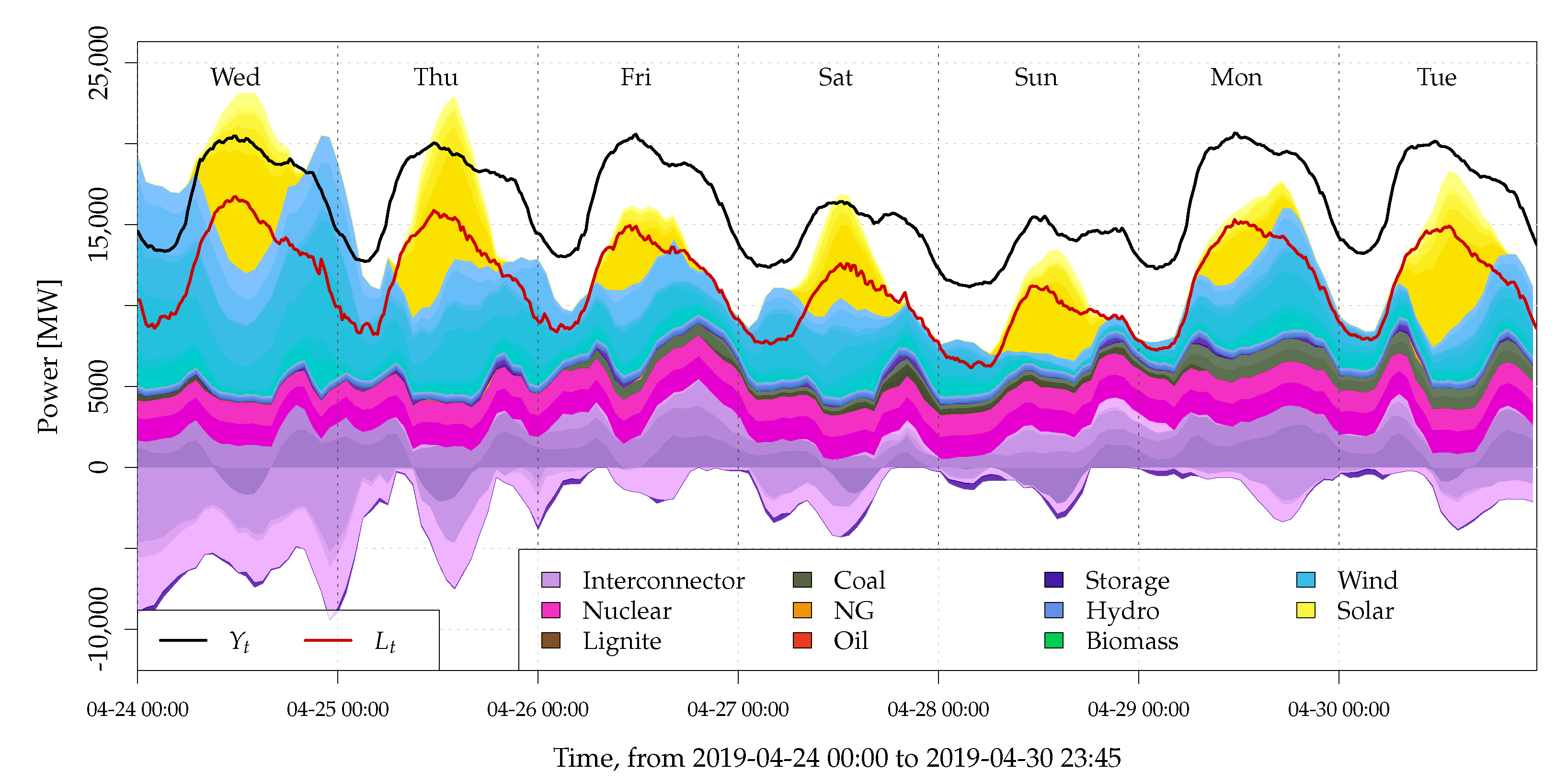
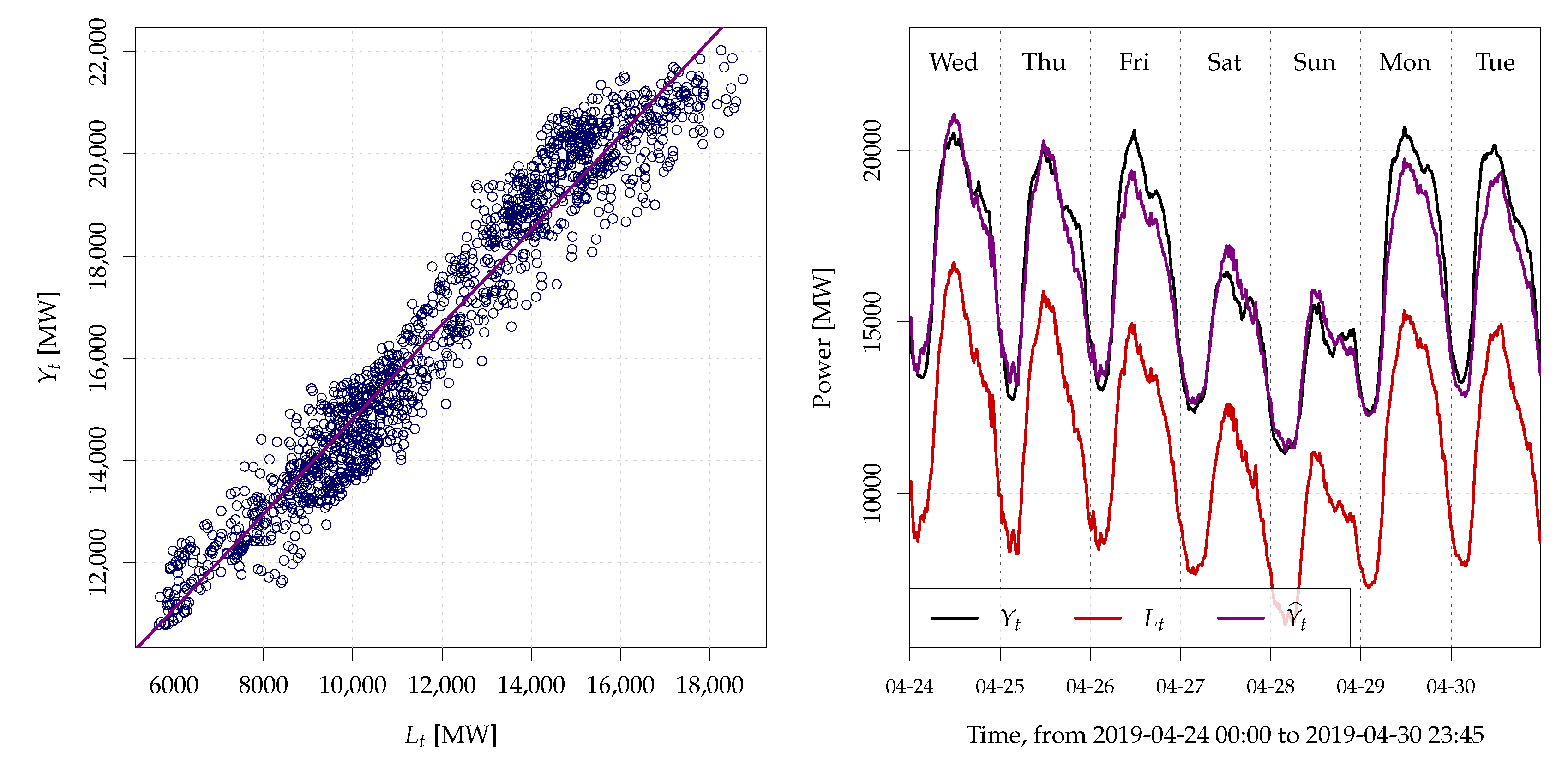
2.2. Data and Problem Illustration

We considered a dataset ranging from 31 December 2014 to 30 April 2019 for the region of a European system operator. The data were metered in quarter-hourly resolution, and if not stated otherwise, all load values are given in MW. There were ${\mathcal{J}}_G=92$ generation time series and ${\mathcal{J}}_I=5$ five interconnection balance time series available. The generation time series contained seven wind power series and five solar series and a diverse collection of power plant productions of different types: nuclear, lignite, coal, natural gas (NG), oil, pump storage, hydro, and biomass. Potential missing data were replaced by the last known values. Moreover, we applied clock change adjustments to the data due to daylight savings time. Hence, for the last Sunday in March, we interpolated the missing clock change hour, and for the last Sunday in October, we averaged the doubling clock change hour.

In Figure 1, we illustrate an example of the considered dataset for the last week of April 2019. We observed that the load process $Y_t$ exhibited the typical daily pattern with smaller values during night than during day time, and smaller values on the weekend than on working days. Additionally, we see that the process $L_t$ (see Equation (3)) is the sum of all available meters series $X_{G,i,t}$ and $X_{I,i,t}$. Note that metering data exhibited negative values, and this held particularly for the transmission data of the interconnectors and the storages. Thus, only if all metered data were positive, the process $L_t$ was visually that of all individual generation and interconnector data. Such a particular example period can be spotted for the last hours of Sunday in Figure 1.

Further, we observed that during the illustrated period, the generation had a substantial infeed of wind and solar power. Additionally, we see that nuclear power provided base load energy, but also some coal power plants in the last two days of April 2019. The remaining power plant contributed only little to the energy supply during this period. Finally, we want to highlight that $L_t$ followed the same pattern as $Y_t$, but lied consistently below $Y_t$. This also motivated the first simple model for predicting $Y_t$.

3. Nowcasting Models

3.1. Benchmark Model

The industry benchmark from the system operator solves the problem stated above by a linear regression on $L_t$ motivated by Equation (2). Thus,

$$Y_t={\alpha }_0+{\alpha }_1{L}_t+{\epsilon }_t$$

(4)

To estimate the unknown coefficients ${\alpha }_0$ and ${\alpha }_1$, the industry benchmark applies ordinary least squares (OLS) to the past years data of the same month of the target time t. Thus, if we want to predict $Y_t$, which is in January, we take all January values for $Y_t$ and $L_t$ of the previous year to estimate ${\alpha }_0$ and ${\alpha }_1$. As we had quarter-hourly data, this was $31\times 96$ data points. By OLS, we used ${\widehat{\alpha }}_0$ and ${\widehat{\alpha }}_1$ and computed nowcasts $Y_t$ by ${\widehat{Y}}_t={\widehat{\alpha }}_0+{\widehat{\alpha }}_1{L}_t$.

The estimation principle is visualized in Figure 2. Here, ${\alpha }_0$ and ${\alpha }_1$ of Model (4) were estimated using the input data from April 2018 for estimating $Y_t$ in April 2019. Note that we will generalize this estimation method slightly and consider a broader range of training periods options in the application.

3.2. Proposed Nowcasting Model

The proposed model was motivated by Equation (3). First, we imposed a linear model on the individual generation and interconnector components by:

$$\begin{array}{cc}\hfill Y_t& ={\beta }_0+\sum _{i=1}^{{\mathcal{J}}_G}{\beta }_{G,i}{X}_{G,i,t}+\sum _{i=1}^{{\mathcal{J}}_I}{\beta }_{I,i}{X}_{I,i,t}+{\epsilon }_t\hfill \end{array}$$

(5)

$$\begin{array}{cc}\hfill & ={\beta }_0+{\beta }_G^{\prime }{\mathit{X}}_{G,t}+{\beta }_I^{\prime }{\mathit{X}}_{I,t}+{\epsilon }_t\hfill \end{array}$$

(6)

$$\begin{array}{cc}\hfill & ={\beta }_0+{\beta }_F^{\prime }{\mathit{X}}_{F,t}+{\epsilon }_t.\hfill \end{array}$$

(7)

with ${\mathit{X}}_{F,t}=({\mathit{X}}_{G,t},{\mathit{X}}_{I,t})$. We regarded this as a fundamental linear load model, as the only linear inputs were ${\mathit{X}}_F$, which contained all fundamental information: the generated power data ${\mathit{X}}_{G,t}$ and the interconnector imbalance ${\mathit{X}}_{I,t}$. Note that (7) can be regarded as natural extension of (4) because Model  (7) turns into (4) by choosing ${\beta }_i={\alpha }_1$ for $i>0$.

However, we extended Model (7) by two further terms: (i) a term that contains seasonal information and (ii) a term that represents autoregressive information. In load forecasting, both terms showed high relevance; see, e.g., [10,11,12,13]. Sometimes, models with many seasonal and autoregressive components performed even very well in short-term forecasting; see, e.g., [14].

Formally, the extended model is given by:

$$\begin{array}{cc}\hfill Y_t& ={\beta }_0+{\beta }_F^{\prime }{\mathit{X}}_{F,t}+{\beta }_S^{\prime }{\mathit{X}}_{S,t}+{\beta }_A^{\prime }{\mathit{X}}_{A,t}+{\epsilon }_t.\hfill \end{array}$$

(8)

$$\begin{array}{cc}\hfill & ={\beta }_0+{\beta }^{\prime }{\mathit{X}}_t+{\epsilon }_t\hfill \end{array}$$

(9)

where ${\mathit{X}}_{S,t}$ is a vector of seasonal regressors and ${\mathit{X}}_{A,t}$ is a vector of autoregressive components of $Y_t$. Of course, (8) turns into (7) by choosing ${\beta }_S=0$ and ${\beta }_A=0$. Note that we also defined ${\mathit{X}}_t=({\mathit{X}}_{F,t},{\mathit{X}}_{S,t},{\mathit{X}}_{X,t})$, which did not include the intercept. Hence, $\beta ={({\beta }_F,{\beta }_S,{\beta }_A)}^{\prime }$ did not include ${\beta }_0$.

It is widely known that in electricity demand, load and consumption modeling periodic features play an important role. The most important seasonalities are daily, weekly, and annual cycles. We suggested to model the three periodic components by periodic cubic by splines with periodicities $S_D$, $S_W$, and $S_A$, which represent a day, a week, and a (meteorologic) year, as in [15]. For out quarter-hourly data, we had $S_D=96$, $S_W=96\times 7=672$, and $S_A=96\times 365.24=$ 35,063.04. In contrast to Fourier analysis, periodic B-splines have the advantage that the basis functions are local and allow for flexibility. When applied to positive data with positivity constraints, they also benefit from the fact that they are always positive. We chose equidistant basis functions for each period. Additionally, we specified the number basis functions $B_D$, $B_W$, and $B_A$ for each period. For our application, we chose $B_D=24$, $B_W=12$, and $B_A=24$. Thus, ${\beta }_S$ had a length of $B_D+B_W+B_A$, which was 60 in our application.

Furthermore, we had to specify the autoregressive term in (8). We defined the autoregressive components:

$${\mathit{X}}_{A,t}=({\left(Y_{t-k}\right)}_{k\in {\mathcal{K}}_{\mathrm{K}}},{\left(Y_{t-k}\right)}_{k\in {\mathcal{K}}_{\mathrm{A}}})$$

with two sets of lags ${\mathcal{K}}_{\mathrm{K}}$ and ${\mathcal{K}}_{\mathrm{A}}$. ${\mathcal{K}}_{\mathrm{K}}$ contained lags around the most recent available $Y_{t-K}$, and ${\mathcal{K}}_{\mathrm{A}}$ contained lags around a calendar year ago. The latter mimicked annual effects.

We specified for the most recent lags:

$${\mathcal{K}}_{\mathrm{K}}=\{K+(0,1,\dots ,8),K+S_D+(-8,-7,\dots ,8),K+2S_D,K+8S_D\}$$

which contains the nine most recent known values, the values eight hours around the day before $Y_{t-K}$, and the lags of the past eight days at the same hour as t. Remember that $K=90S_D$ in our application; thus, $Y_{t-z}$ with $z=K+S_D=91S_D=13\times 7S_D=13S_W$ had the same weekday as the target $Y_t$. For lag around a year ago, we specified:

$${\mathcal{K}}_{\mathrm{A}}=\{50S_W,52S_W+(-8,-7,\dots ,-1,1,2,\dots ,8)S_D,52S_W+(-8,-7,\dots ,8),54S_W\}$$

as $52S_W=364$ is approximately one calendar year. In total, ${\mathcal{K}}_{\mathrm{K}}$ and ${\mathcal{K}}_{\mathrm{A}}$ contributed 54 parameters to the model.

To summarize, the overall (8) had many parameters. In our application scenario, in total, there were $5+12+80+60+54=211$ parameters. As this might lead to overestimation issues when applying plain OLS, we proposed the application of efficient regularization techniques to tackle the nowcasting problem adequately.

3.3. Estimation of Proposed Nowcasting Model

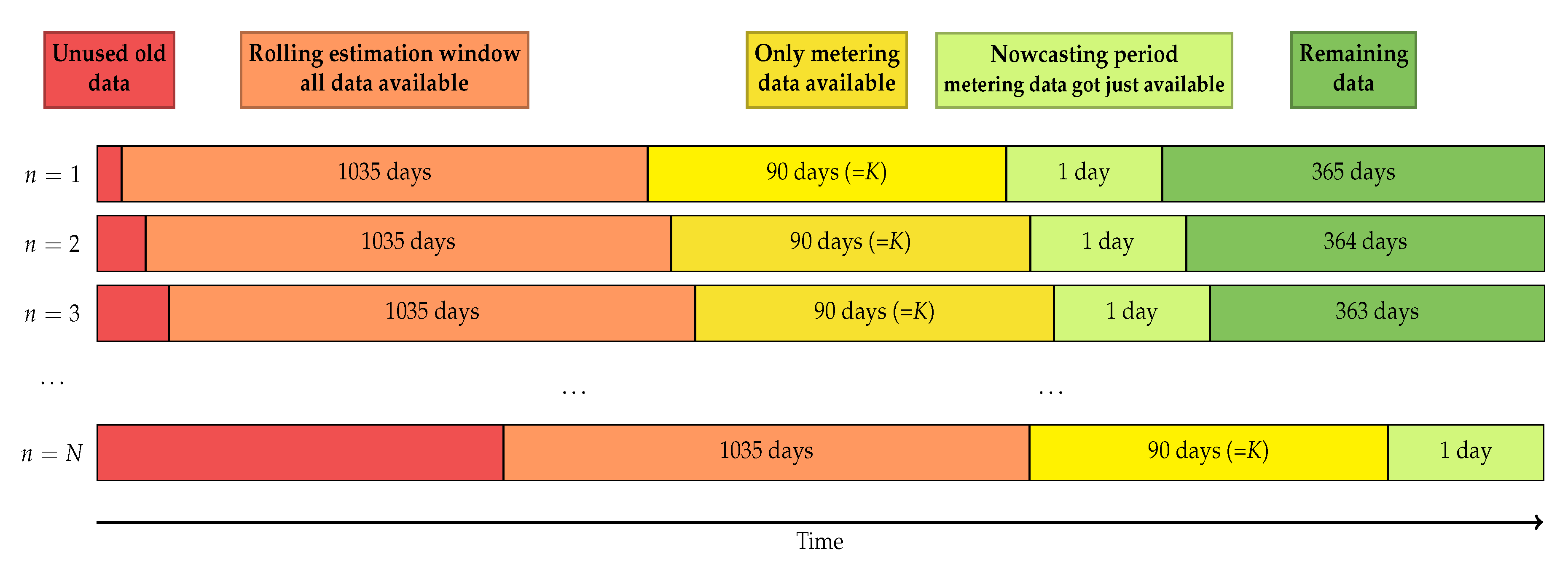
We will see that the estimation procedure (or training method) played an important role in an accurate nowcasting. Obviously, a natural estimation candidate for Model (8) is linear regression. However, as we had many parameters and some of them might contain useless information, this might be suboptimal. Regularization can help to address the problem. In the energy forecasting literature, the lasso (least selection and shrinkage operator) seems to be a popular choice for shrinkage and feature selection methods in linear models; see, e.g., [15,16,17,18]. An extension of the lasso is given by the elastic net, which also has been applied [19,20,21,22,23,24,25].

For introducing the estimation procedure, we require some further notations. Let $\{1,\dots ,T\}$ be the time points of available data for $Y_t$. Thus, our objective was to predict the load $Y_t$ at time point $t=T+K$, which corresponds to the actual time point. Let $\mathbb{T}\subseteq \{1,\dots ,T\}$ be the training period of size $n_{\mathbb{T}}$. Define $\mathbb{Y}(m_0,s_0)={((Y_t-m_0)/s_0)}_{t\in \mathbb{T}}$ as the $(m_0,s_0)$-standardized response vector and $\mathbb{X}(p,{\mathit{s}}_p)={\left({\mathbb{X}}_i(m_i,s_i)\right)}_{i\in \{1,\dots ,p\}}={((X_{i,t}-m_i)/s_i)}_{(i,t)\in \{1,\dots ,p\}\times \mathbb{T}}$ as the scaled input matrix with scaling coefficients $p=(m_1,\dots ,m_p)$ and ${\mathit{s}}_p=(s_1,\dots ,s_p)$ and number of input parameters p. Denote $=(m_0,m_1,\dots ,m_p)$ and $\mathit{s}=(s_0,s_1,\dots ,s_p)$ the collections of all scaling coefficients.

Furthermore, denote $\mathit{c}$ as a vector of the same size as $\beta$, which will be the shrinkage target. In the vast majority of applications, this is $\mathit{c}=0$. The intuition behind this choice is that a specific regressor has zero impact if it contains useless information, to reduce the garbage in, garbage out problem.

With all the notations above, the elastic net estimator for $\beta$ in Model (8) is given as:

$${\widehat{\beta }}_{\lambda ,\alpha }(,\mathit{s};\mathit{c})={\displaystyle \underset{({\beta }_0,\beta )\in {\mathbb{R}}^{p+1}}{arg\; min}}\frac{1}{n_{\mathcal{T}}}{∥\mathbb{Y}(m_0,s_0)-{\beta }_0+{\beta }^{\prime }\mathbb{X}(p,{\mathit{s}}_p)∥}_2^2{+\lambda \alpha \parallel \beta -\mathit{c}\parallel }_1+\lambda \frac{1-\alpha }{2}{\parallel \beta -\mathit{c}\parallel }_2^2$$

(10)

where $\lambda ,\alpha \ge 0$ are tuning parameters, p is the number of parameters (length of $\beta$), and ${\parallel ·\parallel }_1$ and ${\parallel ·\parallel }_2$ as the standard ${\ell }_1$ and ${\ell }_2$ norm. The tuning parameters $\lambda$ and $\alpha$ characterize the regularization properties of the elastic net. For $\alpha =1$, we used the popular choice of the lasso (least absolute shrinkage and selection operator), and for $\alpha =0$, we used the ridge regression, which is also known as Tikhonov regularization. For $\lambda =0$, we used the OLS solution, and for very large $\lambda$, we used a solution very close to the shrinkage target $\mathit{c}$. In the non-ridge case $\alpha >0$, we even used exactly $\mathit{c}$ as the solution if $\lambda$ was sufficiently large. For the case of the ridge regression, we had an explicit solution available. This was:

$${\widehat{\beta }}_{\lambda ,0}(,\mathit{s};\mathit{c})={\left(\tilde{\mathbb{X}}{(p,{\mathit{s}}_p)}^{\prime }\tilde{\mathbb{X}}(p,{\mathit{s}}_p)+Diag\left(\tilde{\lambda }\right)\right)}^{-1}(\tilde{\mathbb{X}}(p,{\mathit{s}}_p)\mathbb{Y}(m_0,s_0)+\lambda \tilde{\mathit{c}})$$

with $\tilde{\mathbb{X}}(p,{\mathit{s}}_p)=(1,\mathbb{X}(p,{\mathit{s}}_p))$, $\tilde{\lambda }={(0,\lambda 1)}^{\prime }$, and $\tilde{\mathit{c}}={(0,\mathit{c})}^{\prime }$. In the elastic net or lasso case with $\alpha >0$, we had efficient estimation techniques based on the coordinate descent or LARS (least angle regression) available. Both options had the drawback that they could only handle the case $\mathit{c}=0$.

However, also the scaling coefficients m and s impacted the estimation substantially. Usually, the scaling coefficients m and s in (10) are standardized so that $\mathbb{Y}({\mathit{m}}_0,{\mathit{s}}_0)$ remains unchanged by $\mathit{m}=0$ and $\mathit{s}=1$, and ${\mathbb{X}}_{\mathit{i}}({\mathit{m}}_{\mathit{i}},{\mathit{s}}_{\mathit{i}})$ has mean zero and standard deviation of one, i.e., it holds that ${\mathbb{X}}_{\mathit{i}}{({\mathit{m}}_{\mathit{i}},{\mathit{s}}_{\mathit{i}})}^{\prime }1=0$ and $\parallel {\mathbb{X}}_{\mathit{i}}({\mathit{m}}_{\mathit{i}},{\mathit{s}}_{\mathit{i}}){\parallel }_2=1$. The latter can be achieved by choosing ${\mathit{m}}_{\mathit{i}}={\mathit{n}}_{\mathbb{T}}^{-1}{\mathbb{X}}_{\mathit{i}}^{\prime }1$ and ${\mathit{s}}_{\mathit{i}}=\sqrt{{\mathit{n}}_{\mathbb{T}}^{-1}{({\mathbb{X}}_{\mathit{i}}-{\mathit{m}}_{\mathit{i}}1)}^{\prime }({\mathbb{X}}_{\mathit{i}}-{\mathit{m}}_{\mathit{i}}1)}$. This scaling procedure is standard in the literature and, e.g., the default in the glmnet or lars packages in R for estimation of the elastic net and lasso estimation with $\mathit{c}=0$.

Still, it turned out that for our nowcasting problem, the scaling procedure for $\mathbb{X}$ was suboptimal as we ignored historic observations. It is true that ${\mathit{Y}}_{\mathit{T}}$ was the last known observation. However, for ${\mathit{X}}_{\mathit{t}}$, we knew all observations up to $\mathit{T}+\mathit{K}$, the time point when the forecast was created. Thus, we proposed to compute the scaling coefficients ${\mathit{s}}_{\mathit{i}}$ and ${\mathit{m}}_{\mathit{i}}$ on the larger and more recent information set ${\mathbb{T}}_{\mathit{K}}=\mathbb{T}\cup \{\mathit{T}+1,\dots ,\mathit{T}+\mathit{K}\}$ for all ${\mathbb{X}}_{\mathit{i}}$. Moreover, we suggested for reasons explained in the next paragraph to scale the $\mathbb{Y}({\mathit{m}}_0,{\mathit{s}}_0)$ by the corresponding sample mean and standard deviation ${\mathit{m}}_0={\mathit{n}}_{\mathbb{T}}^{-1}{\mathbb{Y}}^{\prime }1$ and ${\mathit{s}}_0=\sqrt{{\mathit{n}}_{\mathbb{T}}^{-1}{(\mathbb{Y}-{\mathit{m}}_{0}1)}^{\prime }(\mathbb{Y}-{\mathit{m}}_{0}1)}$.

Now, we discuss the impact of the shrinkage target $\mathit{c}$ in more detail. We mentioned already that the standard choice $\mathit{c}=0$ was motivated by the fact that by default, a regressor has no influence. Only if a regressor contributes substantially to the explanation of the response ${\mathit{Y}}_{\mathit{t}}$, the estimated coefficient will deviate from zero and show a corresponding impact. If we have no further information about our regressors, this is a reasonable approach. We will apply this approach to the ridge and lasso estimator and denote them by 0-ridge and 0-lasso.

However, in our situation, we knew something about the fundamental relationship between our response vector ${\mathit{Y}}_{\mathit{t}}$ and the fundamental regressors ${\mathit{X}}_{\mathit{F},\mathit{t}}$ from Equations (1) and (7). This fundamental relationship could help to impose a suitable regularization for our model. We explain this with the following example: Suppose there is a situation where in the in-sample period or training period $\{0,\dots ,\mathit{T}\}$, a certain power plant or interconnector is offline; thus, all observations are zero. A reason could be that it is a new unit that just started operating somewhere after the last observation known ${\mathit{Y}}_{\mathit{T}}$. Then, the ridge or lasso estimators with $\mathit{c}=0$ will give an estimated coefficient of zero for the corresponding unit. Hence, the power plant will have no out-of-sample contribution to the overall load even though it is operating now, at ${\mathit{Y}}_{\mathit{T}+\mathit{K}}$. Thus, from the fundamental point of view, it makes sense to deviate from the shrinkage target of $0$ for all generation units or interconnectors. If we assume that the metered values are reasonable, eps. not contaminated by implausible data, then taking these values into account should improve the forecasting accuracy. This holds at least for the situation just explained. Hence, we proposed the choice:

$${\mathit{c}}_{\mathit{C}}=({\mathit{c}}_{\mathit{F}},{\mathit{c}}_{\mathit{A},\mathit{S}})$$

with ${\mathit{c}}_{\mathit{F}}=1$ and ${\mathit{c}}_{\mathit{A},\mathit{S}}=0$ corresponding to the impact as in the perfect fundamental situation from Equation (1). Obviously, the vector ${\mathit{c}}_{\mathit{F}}$ had a length of ${\mathit{\beta }}_{\mathit{F}}$, and ${\mathit{c}}_{\mathit{A},\mathit{S}}$ had the aggregated length of ${\mathit{\beta }}_{\mathit{A}}$ and ${\mathit{\beta }}_{\mathit{F}}$. We applied this choice for the ridge regression only and denoted it by c-ridge. The reason why this choice was not applied to lasso or elastic net estimators with $\mathit{\alpha }>0$ was the unavailability of efficient estimation algorithms.

4. Nowcasting Study

We conducted a rolling window nowcasting study using the considered European dataset, and the design was similar to a standard rolling window forecasting study, as illustrated in Figure 3. The initial last known load value ${\mathit{Y}}_{\mathit{T}}$ was on 29 January 2018 at 23:45. Based on historic data, we nowcast the ${\mathit{S}}_{\mathit{D}}=96$ values ${\mathit{Y}}_{\mathit{T}+\mathit{K}+1},\dots ,{\mathit{Y}}_{\mathit{T}+\mathit{K}+{\mathit{S}}_{\mathit{D}}}$. We considered a publication delay of $\mathit{K}=90\times 96=8640$ (90 days), which resulted in the first nowcast being on 30 April 2018, approximately three months later. Then, we shifted the last known load value by a day (${\mathit{S}}_{\mathit{D}}=96$ time points) to ${\mathit{Y}}_{\mathit{T}+{\mathit{S}}_{\mathit{D}}}$ and nowcast ${\mathit{Y}}_{\mathit{T}+\mathit{K}+{\mathit{S}}_{\mathit{D}}+1},\dots ,{\mathit{Y}}_{\mathit{T}+\mathit{K}+2{\mathit{S}}_{\mathit{D}}}$. This procedure was repeated $\mathit{N}=366$ times, which gave an out-of-sample time of about a year and around $96\times 366=$ 35,136 observations for evaluation. For the in-sample dataset, we considered for our application six choices:

(i)

All available data from the past 37 months (three years plus one month):

$(365\times 3+30-90)\times 96=$ 99,360 observations of ${\mathit{Y}}_{\mathit{t}}$, denoted as 3years

(ii)

All available data from the past 25 months (two years plus one month):

$(365\times 2+30-90)\times 96=$ 64,320 observations of ${\mathit{Y}}_{\mathit{t}}$, denoted as 2years

(iii)

All available data from the past 13 months (one year plus one month):

$(365+30-90)\times 96=$ 29,280 observations of ${\mathit{Y}}_{\mathit{t}}$, denoted as 1year

(iv)

Data of the past year, 120 days centered around the nowcasting day of the past year:

$120\times 96=$ 11,520 observations of ${\mathit{Y}}_{\mathit{t}}$, denoted as 4months

(v)

Data of the past year, 60 days centered around the nowcasting day of the past year:

$60\times 96=5760$ observations of ${\mathit{Y}}_{\mathit{t}}$, denoted as 2months

(vi)

Data of the past year, 30 days centered around the nowcasting day of the past year:

$30\times 96=2880$ observations of ${\mathit{Y}}_{\mathit{t}}$, denoted as 1month

Option (i) used the maximum amount of data of $(365\times 3+30-90)=1035$ days, which was also used for illustration in Figure 3. Note that Option (vi) was very close to the industry benchmark approach, which used the data of the month of the previous year for estimating the model parameters.

We considered the all competing models, benchm, 0-lasso ($\mathit{\lambda }$), 0-ridge ($\mathit{\lambda }$), and c-ridge($\mathit{\lambda }$) in the rolling window forecasting study. As emphasized, the lasso and ridge models depended on the tuning parameter $\mathit{\lambda }$, which we had to specify. For all models, we considered exponential grids $\mathsf{\Lambda }$ for $\mathit{\lambda }$; in detail: For the ridge models, we chose $\mathsf{\Lambda }=2^{{\mathcal{L}}_{\mathit{r}}}$ with ${\mathcal{L}}_{\mathit{r}}$ as an equidistant grid from −10 to 20 of length 100, and for the lasso models, $\mathsf{\Lambda }=2^{{\mathcal{L}}_{\mathit{l}}}$ as an equidistant grid from −30 to 3 of length 100. Of course, we did not know in advance the optimal $\mathit{\lambda }$. Therefore, we considered for the 0-lasso, 0-ridge, and c-ridge models a version where $\mathit{\lambda }$ was chosen on the past performance (cumulated loss) of the the corresponding models, initializing with $\mathit{\lambda }=1$ for the first prediction. We denoted the models by 0-lasso${}^{*}$, 0-ridge${}^{*}$, and c-ridge${}^{*}$.

For measuring the nowcasting accuracy or measures for forecasting performance, we considered the out-of-sample MAE (mean absolute error) and the out-of-sample RMSE (root mean square error). To evaluate the forecasting accuracy also for each of the ${\mathit{S}}_{\mathit{D}}=96$ quarter-hours separately, we defined:

$$\begin{array}{cc}\hfill \mathrm{MAE}& =\frac{1}{{\mathit{S}}_{\mathit{D}}}\sum _{\mathit{s}=1}^{{\mathit{S}}_{\mathit{D}}}{\mathrm{MAE}}_{\mathit{s}}\mathrm{with}{\mathrm{MAE}}_{\mathit{s}}=\frac{1}{\mathit{N}}\sum _{\mathit{n}=1}^{\mathit{N}}|{\mathit{Y}}_{\mathit{i},\mathit{s}}-{\widehat{\mathit{Y}}}_{\mathit{i},\mathit{s}}|\hfill \end{array}$$

(11)

$$\begin{array}{cc}\hfill \mathrm{RMSE}& =\frac{1}{{\mathit{S}}_{\mathit{D}}}\sum _{\mathit{s}=1}^{{\mathit{S}}_{\mathit{D}}}{\mathrm{RMSE}}_{\mathit{s}}\mathrm{with}{\mathrm{RMSE}}_{\mathit{s}}=\sqrt{\frac{1}{\mathit{N}}\sum _{\mathit{n}=1}^{\mathit{N}}{|{\mathit{Y}}_{\mathit{i},\mathit{s}}-{\widehat{\mathit{Y}}}_{\mathit{i},\mathit{s}}|}^2}\hfill \end{array}$$

(12)

Note that our models were regression based, and the forecasted value should coincide with the the expected value. Thus, the RMSE should be preferred for evaluation as it identified the true mean correctly. In contrast, the MAE was optimal for median forecasts. However, it is often used as a robust alternative to the RMSE. For more details on the evaluation of point forecasts, we refer to [26].

5. Results

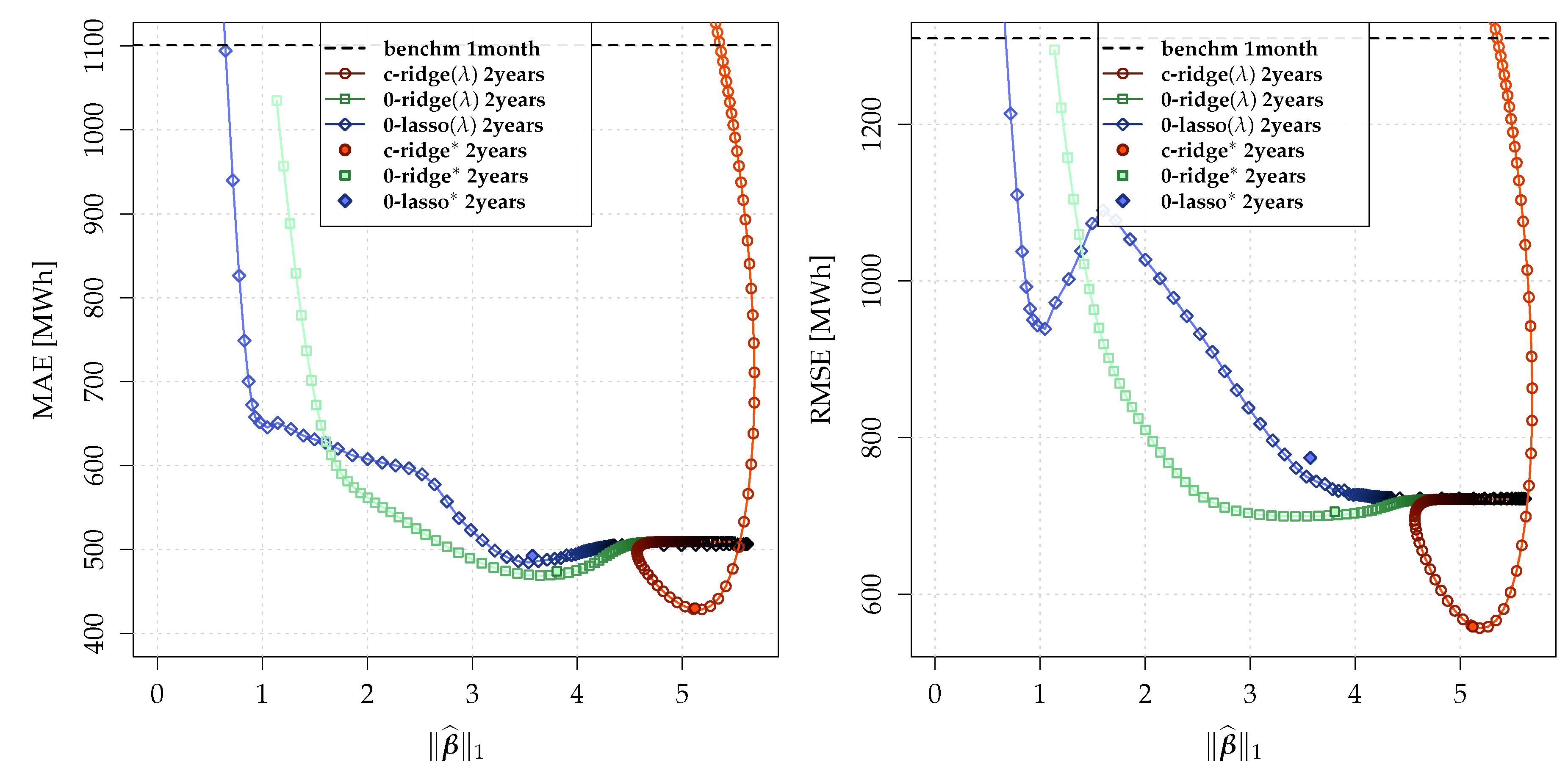
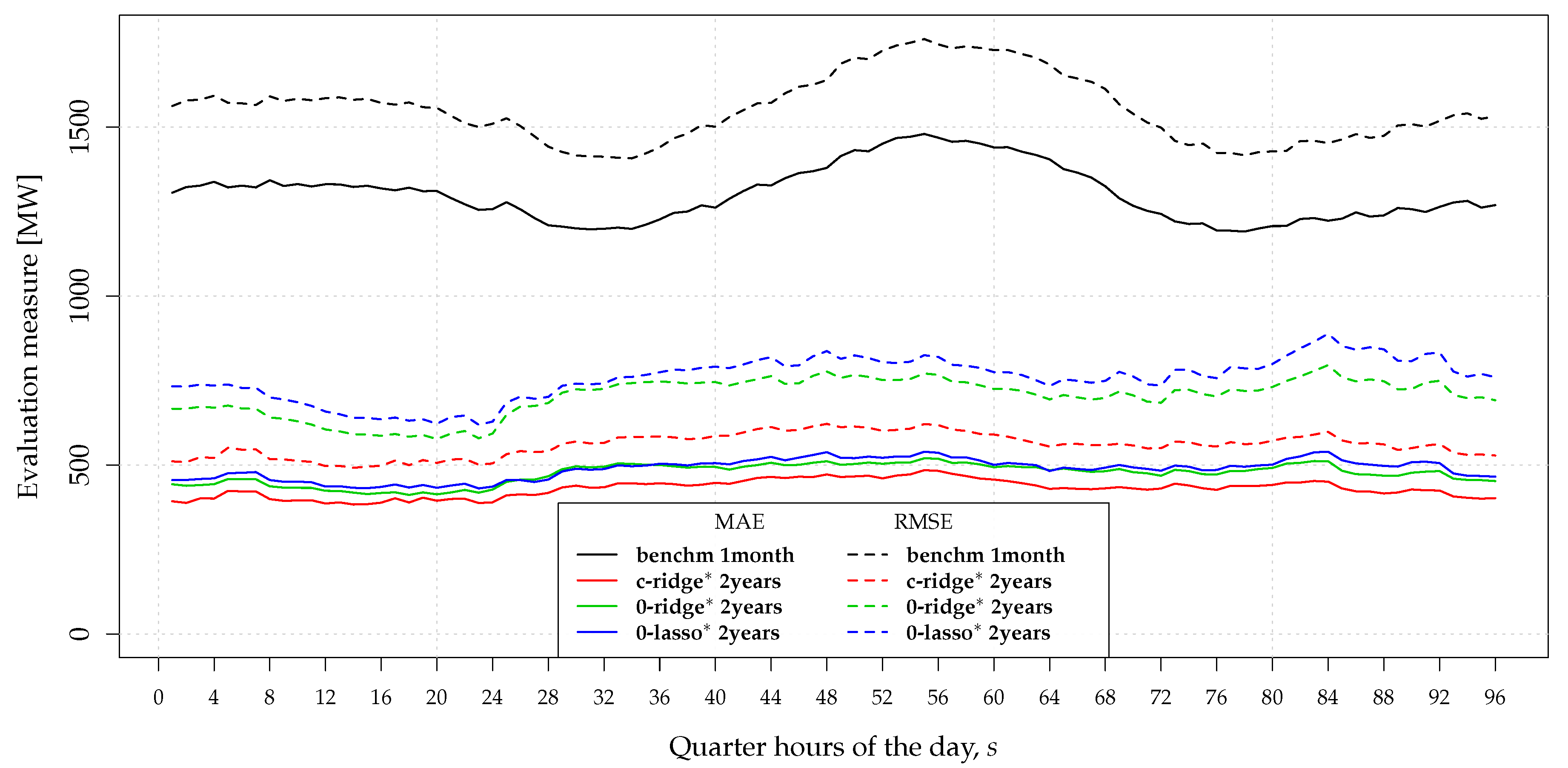
5.1. Nowcasting Performance

We first discuss the overall nowcasting performance of the considered models. The out-of-sample MAE and RMSE values are given in

Table 1. Out-of-sample MAE in MW with relative improvement in % with respect to the benchmark trained on the shortest training period for all models and training periods. A heat map is used to indicate better (→ green) and worse (→ red) performing models.

Models →	benchm		c-ridge${}^{*}$		0-ridge${}^{*}$		0-lasso${}^{*}$		c-ridge		0-ridge		0-lasso
Period↓	MAE	Imp.	MAE	Imp.	MAE	Imp.	MAE	Imp.	MAE	Imp.	MAE	Imp.	MAE	Imp.
3years	1302.7	−18.3	453.6	58.8	483.6	56.1	509.5	53.7	452.1	58.9	481.4	56.3	507.0	53.9
2years	1328.8	−20.7	430.0	60.9	474.1	56.9	487.8	55.7	428.7	61.1	469.0	57.4	484.7	56.0
1year	1290.5	−17.2	653.9	40.6	588.7	46.5	591.0	46.3	630.5	42.7	581.7	47.2	588.8	46.5
4months	1130.2	−2.7	934.3	15.1	549.5	50.1	583.8	47.0	923.2	16.1	538.3	51.1	578.6	47.4
2months	1097.9	0.3	944.5	14.2	602.4	45.3	626.6	43.1	919.6	16.5	593.8	46.1	617.2	43.9
1month	1100.9	0.0	918.0	16.6	607.1	44.9	635.0	42.3	913.1	17.1	604.1	45.1	629.3	42.8

and

Table 2. Out-of-sample RMSE in MW with relative improvement in % with respect to the benchmark trained on the shortest training period for all models and training periods. A heat map is used to indicate better (→ green) and worse (→ red) performing models.

Models →	benchm		c-ridge${}^{*}$		0-ridge${}^{*}$		0-lasso${}^{*}$		c-ridge		0-ridge		0-lasso
Period↓	RMSE	Imp.	RMSE	Imp.	RMSE	Imp.	RMSE	Imp.	RMSE	Imp.	RMSE	Imp.	RMSE	Imp.
3years	1556.0	−18.8	578.9	55.8	710.0	45.8	868.5	33.7	582.2	55.5	713.0	45.6	825.0	37.0
2years	1562.4	−19.3	560.4	57.2	705.1	46.2	759.5	42.0	556.8	57.5	699.5	46.6	721.9	44.9
1year	1460.6	−11.5	1051.3	19.7	858.9	34.4	940.9	28.2	919.9	29.8	817.2	37.6	923.3	29.5
4months	1332.9	−1.8	1185.3	9.5	776.6	40.7	960.9	26.6	1102.3	15.8	754.6	42.4	880.6	32.8
2months	1299.5	0.8	1274.3	2.7	877.1	33.0	975.9	25.5	1121.3	14.4	828.2	36.8	966.9	26.2
1month	1309.7	0.0	1147.9	12.4	850.3	35.1	917.6	29.9	1150.5	12.2	858.2	34.5	914.5	30.2

. There, we also computed improvements in the MAE and RMSE with respect to the benchmark model benchm estimated on the shorted training period 1month. Remember that ridge${}^{*}$ and lasso${}^{*}$ chose the tuning parameter based on the past performance, whereas ridge and lasso represented the models that gave ex-post the best prediction accuracy on the $\mathit{\lambda }$-grid $\mathsf{\Lambda }$.

First, we observe that all ridge and lasso models showed clear improvements against the benchmark. The largest improvement of around 60% in both measures was gained by the c-ridge (or c-ridge${}^{*}$) model calibrated on the training period of 2years. Second, we see that the ridge${}^{*}$ and lasso${}^{*}$ models showed almost the same performance as ridge and lasso, which indicated that the ex-post selection of $\mathit{\lambda }$ was not a big problem. Next, the benchmark model benchm with short calibration periods of 1month and 2months showed the best prediction accuracy against the benchmark model. In contrast, the ridge and lasso approaches showed that long training periods of 2years and 3yearsperformed best. The reason was likely that the estimation of many parameters required more data to receive stable parameter estimates. Figure 4 illustrates the solution path of the ridge and lasso models for a calibration period 2years which uses about two years of data.

Here, the ${\parallel ·\parallel }_1$-norm of $\widehat{\mathit{\beta }}$ as a typical measure for model complexity is plotted against the MAE and RMSE score. Note that $\parallel \widehat{\mathit{\beta }}{\parallel }_1$ is the sum of all absolute parameters. The solution paths for different $\mathit{\lambda }$ values of a certain model e.g., c-ridge ($\mathit{\lambda }$) (red circle), are represented by the color intensity. The darker the color of the symbol within the solution path, the smaller $\mathit{\lambda }$. Thus, black symbols correspond to the OLS solution.

We observe that all three models c-ridge ($\mathit{\lambda }$), 0-ridge ($\mathit{\lambda }$), and 0-lasso ($\mathit{\lambda }$) converged to the the OLS solution for small $\mathit{\lambda }$. The OLS solution had an MAE of around 500 MW and an RMSE of slightly above 700 MW with an ${\parallel ·\parallel }_1$-norm of $\mathit{\beta }$ of around $5.5$. We clearly see that for small $\mathit{\lambda }$ values, 0-ridge ($\mathit{\lambda }$) and 0-lasso ($\mathit{\lambda }$) obtained smaller $\mathit{\beta }$ values and tended towards the $0$ solution. In contrast, c-ridge ($\mathit{\lambda }$) had always a similar range of the ${\parallel ·\parallel }_1$-norm of $\mathit{\beta }$. The corresponding MAE and RMSE minima has a ${\parallel ·\parallel }_1$-norm around 5.2, which is a similar magnitude as the OLS solution. Thus, the parameter complexity of both solutions was comparable, but the parameters were better selected by the c-ridge approach due to the shrinkage towards a reasonable target, instead of $0$.

Next, we wanted to look at the intraday structure of the nowcasting errors across the 96 quarter-hours. The forecasting accuracy in term of MAE${}_{\mathit{s}}$ and RMSE${}_{\mathit{s}}$ is visualized in Figure 5. There, we observe that the benchmarks exhibited a relatively clear diurnal pattern. The nowcasting error was largest during the working hours, esp. during the afternoon. For the lasso and ridge models, the daily pattern was substantially reduced. For instance, the MAE${}_{\mathit{s}}$ of c-ridge${}^{*}$ varied between 383 MW and 484 MW, which was a variation of around 100 MW. The intraday MAE h variation of the MAE of the benchmark model was around 300 MW and significantly larger. However, as the overall forecasting error reduced by 60%, the relative variation of the of the MAE forecasting performance remained at a similar level.

We saw that the proposed models with an in-sample sample size of about two years performed best. It was clear that the computational complexity increased with the amount of data used for training and calibration. Still, in all cases, the models allowed the implementation and application on a real-time basis due to the linear model structure. For instance, the estimation of the c-ridge, 0-ridge, and 0-lasso models on the full $\mathit{\lambda }$-grid with a training period of 2years took $3.0$ s, $0.5$ s, and, $2.3$ s, respectively. These times were measured on a standard computer using a simple CPU. The ridge models were estimated using the solve.QP function of the R package quadprog, and the lasso model was trained and calibrated using glmnet function of the R package glmnet.

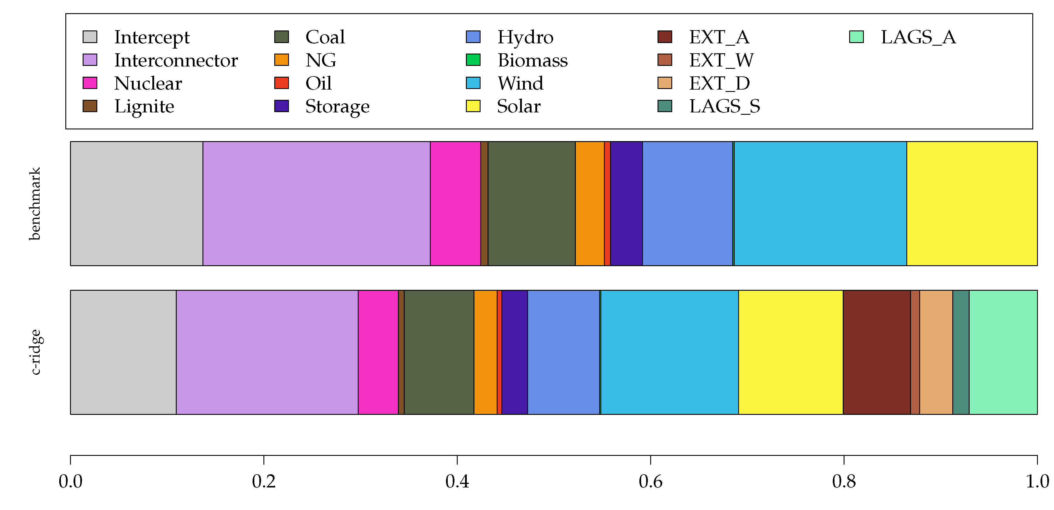
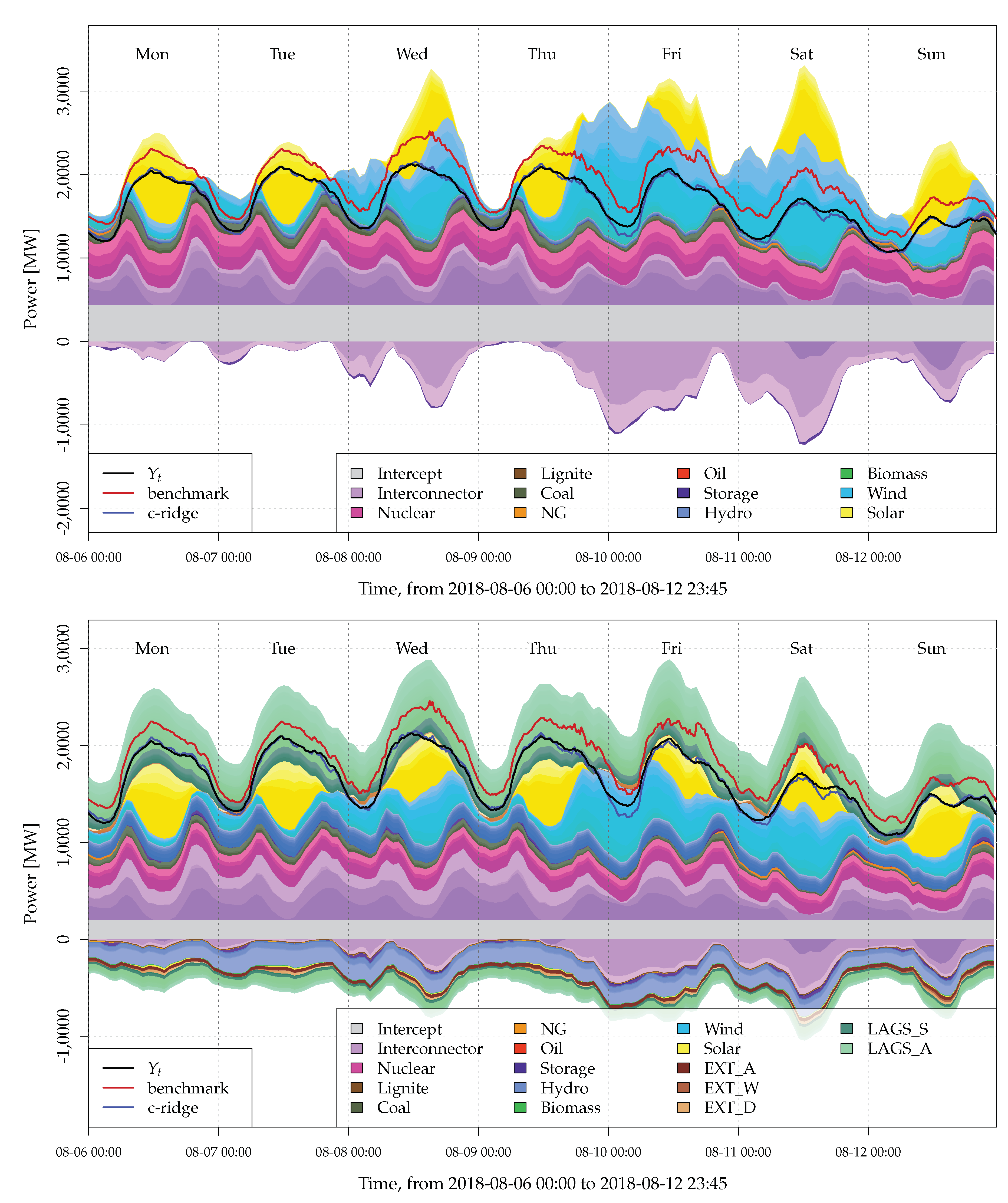
5.2. Model Interpretation

As our models were linear models, it was relatively easy to interpret the parameters. The easiest way to get an understanding of the impact of each parameter in the model was to evaluate the absolute impact of parameter $\mathit{i}$ with respect to the overall parameter contribution $|{\widehat{\mathit{\beta }}}_{\mathit{i}}|/\parallel \widehat{\mathit{\beta }}{\parallel }_1$. Those impacts of the c-ridge${}^{*}$ model with a training period of about two years such as the benchmark model benchm with training period of about a month are illustrated in the bar chart in Figure 6. As the full model had many parameters, we grouped the impacts $|{\widehat{\mathit{\beta }}}_{\mathit{i}}|/\parallel \widehat{\mathit{\beta }}{\parallel }_1$ by parameter type to maintain readable results.

Obviously, we saw that the only the c-ridgemodel had a contribution from external regressors and autoregressive impacts (EXT_A, EXT_W, and EXT_D represent the annual, weekly, and daily seasonal components; LAGS_A and LAGS_S represent the annual and short-term autoregressive lags), as the benchmark model did not take those effects into account. Here, it seemed that the annual impacts contributed substantially to the c-ridge${}^{*}$ model, and this held for both types’ effects from deterministic external regressors (EXT_A) and autoregressive effects (LAGS_A). Furthermore, the daily seasonal component (EXT_D) showed about a 3.5% contribution to the overall solution. For the generation units, we observed that all reduced their absolute impact in the c-ridge${}^{*}$ model with respect to the benchmark model. However, all parameters remained relevant.

The interpretation by the absolute impacts $|{\widehat{\mathit{\beta }}}_{\mathit{i}}|/\parallel \widehat{\mathit{\beta }}{\parallel }_1$ was suitable for evaluation of the impact within the estimated model. However, the regressors ${\mathit{X}}_{\mathit{i},\mathit{t}}$ lived on completely different scales. To obtain interpretable impacts with respect to the load ${\mathit{Y}}_{\mathit{t}}$, we had to evaluate the time series of ${\widehat{\mathit{\beta }}}_{\mathit{i}}{\mathit{X}}_{\mathit{i},\mathit{t}}$, which represented the impact of each single component to the final model. Therefore, Figure 7 shows a time series plot of the actual load ${\mathit{Y}}_{\mathit{t}}$, the benchmark model benchm nowcasts, and the c-ridge${}^{*}$ model nowcasts, along with the estimated contributions ${\widehat{\mathit{\beta }}}_{\mathit{i}}{\mathit{X}}_{\mathit{i},\mathit{t}}$ for each regressor $\mathit{i}$.

We observed that for both models, the interconnector, wind, and solar contributed substantially to the final solution. For the c-ridge${}^{*}$ nowcast, a very important contribution to ${\widehat{\mathit{Y}}}_{\mathit{t}}$ came from the annual autoregressive impacts (LAG_A). It mainly had positive contributions, but also some negative contributions. For the c-ridge${}^{*}$ nowcast, some moderate impact could be seen from the nuclear power and hydro. The latter contributed more to the negative side than to the positive, which was a bit surprising, as the fundamental model would suggest a positive impact. Furthermore, the benchmark model had no negative contribution from hydro power. All other generation types had only a minor impact for both considered models. Finally, we observed that the intercept contributed around 2000 MW to the final contribution of the c-ridge${}^{*}$ model, which was about 10% of the overall load ${\mathit{Y}}_{\mathit{t}}$. Remember that about 80% of the load ${\mathit{Y}}_{\mathit{t}}$ was metered (by generation units and interconnectors). Thus, from the missing 20% load, around a half (=10%) seemed to be base load.

6. Summary and Conclusions

We formally introduced the problem of load nowcasting to the energy forecasting literature. In contrast to load forecasting, the recent load of a certain balancing area was predicted based on limited available metering data within this area. Thus, we were predicting the recent past. We introduced an industry benchmark model and multiple high-dimensional linear model to tackle the nowcasting problem. The model design orientated from load forecasting problems. Next to the impacts of metered generation and interconnector units, the models had seasonal and autoregressive components to improve the prediction performance. We considered multiple estimation techniques based on lasso and ridge and studied the impact of the choice of the training/calibration period.

The overall results showed that in comparison to the industry benchmark, an accuracy improvement in terms of MAE and RMSE of about 60% was achieved. The best model was based on the ridge estimator and used a specific non-standard shrinkage target. Moreover, we highlighted that the model parameters could be interpreted. The overall results showed that the annual effects (deterministic and autoregressive) contributed significantly to the proposed ridge model.

Future research could investigate more nowcasting models, especially non-linear ones, like artificial neural networks or support vector machines. Obviously, the study could be extended to probabilistic nowcasting. The considered nowcasting models could also serve a basis for the construction of load forecasting models. Here, the generation and interconnector units ${\mathit{X}}_{\mathit{i},\mathit{t}}$ had to be considered in a lagged manner (${\mathit{X}}_{\mathit{i},\mathit{t}-\mathit{k}}$), potentially for multiple lags. In general, many methodologies can be transferred from energy forecasting, especially from short-term load forecasting.

Finally, the model accuracy might be enriched by the use of more external information. In load forecasting, the (average) temperature of a objective area is often seen as highly relevant. Thus, the incorporation into a nowcasting model could be beneficial as well. This information can be added easily by adding the temperature (and potential non-linear transformations) as a new regressor to the model. We can also add further dummy variables that characterize known structural breaks, e.g., for changes in the regulation or reshaping of the balancing area. Furthermore, it was clear that additional metering information would improve the nowcasting accuracy. With respect to renewable energy information from wind and solar power, a finer geographical resolution might improve the forecasting accuracy, as Figure 7 shows a high importance for a few individual time series of the c-ridge${}^{*}$ model with respect to the benchmark model.

References

1. Hong, T.; Fan, S. Probabilistic electric load forecasting: A tutorial review. Int. J. Forecast. 2016, 32, 914–938. [Google Scholar] [CrossRef]
2. Schumacher, M.; Hirth, L.; How Much Electricity Do We Consume? A Guide to German and European Electricity Consumption and Generation Data (2015). FEEM Working Paper No. 88.2015. Available online: https://ssrn.com/abstract=2715986orhttp://dx.doi.org/10.2139/ssrn.2715986 (accessed on 20 December 2019).
3. Hirth, L.; Mühlenpfordt, J.; Bulkeley, M. The ENTSO-E Transparency Platform—A review of Europe’s most ambitious electricity data platform. Appl. Energy 2018, 225, 1054–1067. [Google Scholar] [CrossRef]
4. Gerbec, D.; Gubina, F.; Toros, Z. Actual load profiles of consumers without real time metering. In Proceedings of the IEEE Power Engineering Society General Meeting, San Francisco, CA, USA, 12–16 June 2005; IEEE: Piscataway, NJ, USA, 2005; pp. 2578–2582. [Google Scholar]
5. Banbura, M.; Giannone, D.; Reichlin, L. Nowcasting. Available online: https://papers.ssrn.com/sol3/papers.cfm?abstract_id=1717887 (accessed on 20 December 2019).
6. Sun, J.; Xue, M.; Wilson, J.W.; Zawadzki, I.; Ballard, S.P.; Onvlee-Hooimeyer, J.; Joe, P.; Barker, D.M.; Li, P.W.; Golding, B.; et al. Use of NWP for nowcasting convective precipitation: Recent progress and challenges. Bull. Am. Meteorol. Soc. 2014, 95, 409–426. [Google Scholar] [CrossRef] [Green Version]
7. Xingjian, S.; Chen, Z.; Wang, H.; Yeung, D.Y.; Wong, W.K.; Woo, W.c. Convolutional LSTM network: A machine learning approach for precipitation nowcasting. In Advances in Neural Information Processing Systems; Curran Associates, Inc.: Dutchess, NY, USA, 2015; pp. 802–810. [Google Scholar]
8. Sanfilippo, A. Solar Nowcasting. In Solar Resources Mapping; Springer: Cham, Switzerland, 2019; pp. 353–367. [Google Scholar]
9. Sala, S.; Amendola, A.; Leva, S.; Mussetta, M.; Niccolai, A.; Ogliari, E. Comparison of Data-Driven Techniques for Nowcasting Applied to an Industrial-Scale Photovoltaic Plant. Energies 2019, 12, 4520. [Google Scholar] [CrossRef] [Green Version]
10. Gaillard, P.; Goude, Y.; Nedellec, R. Additive models and robust aggregation for GEFCom2014 probabilistic electric load and electricity price forecasting. Int. J. Forecast. 2016, 32, 1038–1050. [Google Scholar] [CrossRef]
11. Ziel, F. Modeling public holidays in load forecasting: A German case study. J. Mod. Power Syst. Clean Energy 2018, 6, 191–207. [Google Scholar] [CrossRef] [Green Version]
12. Ziel, F. Quantile regression for the qualifying match of GEFCom2017 probabilistic load forecasting. Int. J. Forecast. 2019, 35, 1400–1408. [Google Scholar] [CrossRef] [Green Version]
13. Kanda, I.; Veguillas, J.Q. Data preprocessing and quantile regression for probabilistic load forecasting in the GEFCom2017 final match. Int. J. Forecast. 2019, 35, 1460–1468. [Google Scholar] [CrossRef]
14. Haben, S.; Giasemidis, G.; Ziel, F.; Arora, S. Short term load forecasting and the effect of temperature at the low voltage level. Int. J. Forecast. 2019, 35, 1469–1484. [Google Scholar] [CrossRef] [Green Version]
15. Ziel, F.; Liu, B. Lasso estimation for GEFCom2014 probabilistic electric load forecasting. Int. J. Forecast. 2016, 32, 1029–1037. [Google Scholar] [CrossRef] [Green Version]
16. Dudek, G. Pattern-based local linear regression models for short-term load forecasting. Electr. Power Syst. Res. 2016, 130, 139–147. [Google Scholar] [CrossRef]
17. Takeda, H.; Tamura, Y.; Sato, S. Using the ensemble Kalman filter for electricity load forecasting and analysis. Energy 2016, 104, 184–198. [Google Scholar] [CrossRef]
18. Wang, Y.; Gan, D.; Zhang, N.; Xie, L.; Kang, C. Feature selection for probabilistic load forecasting via sparse penalized quantile regression. J. Modern Power Syst. Clean Energy 2019, 7, 1200–1209. [Google Scholar] [CrossRef] [Green Version]
19. Uniejewski, B.; Nowotarski, J.; Weron, R. Automated variable selection and shrinkage for day-ahead electricity price forecasting. Energies 2016, 9, 621. [Google Scholar] [CrossRef] [Green Version]
20. Ambach, D.; Croonenbroeck, C. Space-time short-to medium-term wind speed forecasting. Stat. Methods Appl. 2016, 25, 5–20. [Google Scholar] [CrossRef]
21. Liu, W.; Dou, Z.; Wang, W.; Liu, Y.; Zou, H.; Zhang, B.; Hou, S. Short-term load forecasting based on elastic net improved GMDH and difference degree weighting optimization. Appl. Sci. 2018, 8, 1603. [Google Scholar] [CrossRef] [Green Version]
22. Kath, C.; Ziel, F. The value of forecasts: Quantifying the economic gains of accurate quarter-hourly electricity price forecasts. Energy Econ. 2018, 76, 411–423. [Google Scholar] [CrossRef] [Green Version]
23. Narajewski, M.; Ziel, F. Econometric modelling and forecasting of intraday electricity prices. J. Commod. Mark. 2019, 100107. [Google Scholar] [CrossRef] [Green Version]
24. Pirbazari, A.M.; Chakravorty, A.; Rong, C. Evaluating feature selection methods for short-term load forecasting. In Proceedings of the 2019 IEEE International Conference on Big Data and Smart Computing (BigComp), Kyoto, Japan, 27 February–2 March 2019; IEEE: Piscataway, NJ, USA, 2019; pp. 1–8. [Google Scholar]
25. Muniain, P.; Ziel, F. Probabilistic forecasting in day-ahead electricity markets: Simulating peak and off-peak prices. Int. J. Forecast. 2020. [Google Scholar] [CrossRef] [Green Version]
26. Gneiting, T. Making and evaluating point forecasts. J. Am. Stat. Assoc. 2011, 106, 746–762. [Google Scholar] [CrossRef] [Green Version]
Figure 1. Time series plot of the load Y t and the process L t with its single components X G , i , t and X I , i , t classified by generation type in the last week of April 2019.
Energies 13 01443 g001
Figure 2. (Left) Scatter plot of the process L t (see (3)) and load Y t in April 2018 with the fitted line of Model (4). (Right) Time series plot of Y t , L t , and Y ^ t = α ^ 0 + α ^ 1 L t for the last week of April 2019 as in Figure 1.
Energies 13 01443 g002
Figure 3. Illustration of the nowcasting study design.
Energies 13 01443 g003
Figure 4. Graph of β ^ 1 against MAE (left) and RMSE (right) of the selected lasso and ridge models, illustrating the solution paths for different λ values. The darker the color, the smaller the shrinkage (black = OLS).
Energies 13 01443 g004
Figure 5. Intraday prediction accuracy in MAE s and RMSE s of selected models.
Energies 13 01443 g005
Figure 6. Bar chart of the absolute impact | β ^ i | / β ^ 1 of Model c-ridge * for 2years and benchm for 1month grouped by parameter type.
Energies 13 01443 g006
Figure 7. Time series plot of the actual load Y t (black), with the fitted model of the benchmark model (red) and the c-ridge * approach (blue) on 6–12 August 2018. Additionally, the estimated impact of the single components β ^ i X i , t for the c-ridge * model (bottom) and benchmark model (top) classified by type with different colors is illustrated.
Energies 13 01443 g007