Abstract
This article examines the asymmetric relationship between electric consumption, economic growth, and carbon dioxide emission in 15 countries over the period 1971–2014. We employed a nonlinear auto-regressive distribution Lag (NARDL) model approach to investigate the asymmetric cointegration between variables. Additionally, we applied the asymmetric causality approach to determine the causal relationship between variables. Results confirm nonlinear cointegration between variables in Cameroon, Congo Republic, Zambia, Canada, and the UK. The Wald test results confirm a long-run asymmetric link between electricity consumption, economic growth, and carbon emission in Canada and Cameroon, while a short-run asymmetric effect in the Congo Republic and the UK. Findings from the granger causality test are volatile across variables. The result provides strong support for the symmetric relationship between electric consumption, economic growth, and carbon emission in the short and long run. This study provides new evidence for policymakers to formulate country-specific policies to obtain better environmental quality while achieving sustainable economic growth.
1. Introduction
Greenhouse gas emission (GHG) in the atmosphere poses a severe threat to sustainable development as its impact affects climate change globally in numerous ways like ecosystem destruction and the melting of polar ice, causing a rise in sea levels. It also causes temperature increase leading to disasters like floods and drought. The main component of this GHG is carbon dioxide (CO2) emission. For some decades now, the topic of the causal relationship between the impact of CO2 emission on gross domestic products (GDP) and electric consumption (ECON) has been of high interest among researchers [1,2]. Some factors like increased electricity demand and services, goods and economic growth have led to the increase in CO2 emissions especially in the sub-Saharan region of Africa over the decades [3] which has a high population of close to 1 billion people and has the most inadequate access to electricity [4]. World Development Indicators show that CO2 emissions for some years now have been on the increase due to electricity transmission, which has led to a decrease inefficiency of the power sector. Algeria, which is not part of the sub-Saharan countries, is the third-highest emitter of CO2 in Africa [5]. Additionally, the G7 countries have 47% of the global GDP, and these countries are rated as the part of the world’s advanced economies attached to the energy–growth relationship which impacts on energy consumption, economic growth and has led to climate change response strategies. To help combat these consequences of CO2 emission, many countries, both developing and developed countries, have signed the Kyoto Protocol aimed at reducing carbon emission globally [6].
As early as the 1970s, some scholars started researching the relationship between carbon emission, electric consumption, and gross domestic product [7]. Numerous studies have checked the Environmental Kuznets Curve (EKC) that analyzes the environmental quality and economic growth. According to the EKC hypothesis, environmental degradation transitions from an upward trend to a downward trend once the economic level reaches a certain threshold. If carbon emissions increase with economic growth, economic development still occurs at the expense of the environment. It goes ahead to say that environmental degradation increases firstly then starts to reduce as growth per capita continues to rise. The link between energy consumption, economic growth, and carbon emission has undoubtedly ranked first among the studies common in the empirical energy economics literature [6,8,9,10].
Most previous studies on the energy-carbon-economy have focused on the relationship between economic growth and carbon emission or energy consumption in a linear framework. However, the variations in the findings have failed to provide a consistent solution for policymakers. A comprehensive literature review can be seen in Table 1.

Table 1.
Empirical studies on the relationships between CO2 emissions, energy consumption, and economic growth.
Based on a comparative analysis between developing and developed countries on the relationship between carbon dioxide emission, energy consumption, and economic growth by [18] based on panel data from 1971–2014 using an ordinary least squares method, the results confirm a high correlation between CO2, GDP, energy consumption, energy intensity, and trade openness. The results do not support the EKC hypothesis. The authors of [19] investigated the existence of the Environmental Kuznets Curve (EKC) in China from 1970 to 2015. The ARDL (Autoregressive Distributed Lag) model, FMOLS (Fully Modified Ordinary Least Squares), DOLS (Dynamic Ordinary Least Squares), impulse response and variance decomposition models were employed to examine the nexus between CO2 emissions, economic growth, and energy consumption. The result supports the Environmental Kuznets Curve (EKC) hypothesis from different techniques; long-run economic growth in favor of environmental quality was confirmed. In [20] the authors used a panel cointegration and vector error-correction model to discuss the dynamic economy–energy–environment nexus for 188 countries for the period of 1993–2010. Results show the existence of long-run relationships between economic growth, energy consumption, and CO2 emissions for all countries; energy consumption negatively affects GDP worldwide as a whole; unidirectional causality from energy consumption to carbon dioxide emissions exists. They investigated the effects on the economy of a feed-in-tariff policy mechanism aimed to foster investments in renewable energy production. The authors of [21] employed a Eurace macroeconomic model. Findings confirm that the feed-in tariff policy was effective in promoting the sustainability transition of the energy sector and that it increases investment level with a positive impact on the unemployment rates. Additionally, it was observed that GDP increases the share of the investment sector in the economy, due to the building-up of renewable production capacity, with a resulting crowding out of consumption, higher rates, and prices.
Over the years, many researchers have investigated the nexus between energy consumption, carbon emissions, and economic growth, without a consensus. Due to the mixed results, many countries have been put in a difficult situation when formulating and adopting energy policies [22]. The diversity in recent findings is as a result of the different methodologies applied, the different time frames, and diverse countries studied according to [23].
This study contributes to existing literature, majorly in the field of energy and ecology. Firstly, instead of using a sample that only includes a single type of country, this study selects a heterogeneous sample composed of both developed and developing countries. Six out of the seven G7 constituting developed and industrialized countries in the world, namely Canada, France, Italy, Japan, the UK, and the US, were studied. Additionally, we assessed eight African countries making up our sample for developing nations, namely: Algeria, Cameroon, Congo Democratic Republic, Congo Republic, Ghana, Kenya, Nigeria, Zambia, and India. Given this, a diverse sample is necessary and useful for country-specific energy policymaking and formulation.
Secondly, this study utilizes the recently developed nonlinear autoregressive distributed lag model (NARDL) developed by [24]. The nonlinear ARDL is very important to explain the asymmetric relationship that exists between electric consumption, economic growth, and carbon emission. Unlike other models applied in previous studies, the NARDL allows testing the long run and short run asymmetries in the variables. The bounds testing approach exhibits robustness to small sample sizes and concurrently identifying asymmetries existing in the dynamic adjustment allowing regressors of mixed order I(0) and I(1) [24,25,26].
Thirdly, the study incorporates the nonlinear Granger causality presented in [27] instead of the widely used nonlinear causality test presented in [28] to examine the causality relationship between electric consumption, economic growth, and carbon emission in a nonlinear framework. In [27] the nonlinear Granger causality was adopted as a result of the shortcomings pointed out by Dicks and Panchenko in the Hiemstra and Jones test that it may over reject the null hypothesis of noncausality.
2. Data and Methodology
2.1. Data
The data used in this research is from the World Bank Development Indicators (WDI). Annual data was used that covers a period of 44 years, from 1971 to 2014, based on the availability of data. The multivariate framework included CO2 emissions (CE) (measured metric tonne per capita) as our dependent variable, gross domestic product (GDP) per capita current 2010 US dollars (as a proxy for economic growth) (EG), and electric power consumption KW per capita (EC). All variables were converted into logarithms before analysis. Summary statistics are provided in Table 2.

Table 2.
Summary statistics.
2.2. Methodology
This study investigates the relationship that exists between electricity consumption, economic growth, and carbon emission using a nonlinear (asymmetric) approach to determine the short- and long-run asymmetric relationships.
where i represents the countries and years, log denotes logarithm. CE denotes carbon emission, EC represents electric consumption, and EG is economic growth.
We adopted the nonlinear ARDL bounds testing approach developed by [29], which considers nonlinear and asymmetric cointegrations between variables. Additionally, it differentiates the long-run effects and short-run effects of the independent variables on the dependent variables. It is applicable irrespective of whether the variable is stationary at the level, or first difference l(0) or l(1) provided none of these variables is l(2) by [30]. This article employs this NARDL cointegration to investigate the relationship between carbon emission (CO), electric consumption (EC), and gross domestic product (EG). This method enables us to determine the functional relationship between carbon emission, electric consumption, and gross domestic products.
From the first equation, depicts long-run coefficients, depicts short-run coefficients, with i = 1….8. Long-run coefficients give the reaction time and speed time of the adjustment towards the equilibrium level. At the same time, the immediate effect of independent variables on dependent variables were determined using the short-run. We used the Wald test to determine the short-run asymmetry () and long-run asymmetry ( for variables where is electric power consumption, represents GDP per capita, and represents CO2 emission. Dt denotes a dummy variable used to know the impact of the break date (t). The Akaike information criterion (AIC) helps to determine p and q, which are the optimal lags for the independent variables () and the dependent variable .
Decomposing the independent variables into positive and negative sums, we have
To conduct a combined test for all lagged levels of regressors, we performed a proposed bound test by [29] to check whether an asymmetric long-run cointegration exists. We applied two tests in this part of the article namely F-statistics the null hypothesis of against alternative hypothesis by [26] and T- statistics by [31] in this the null hypothesis tests the null hypothesis at against alternative hypothesis . To estimate long-run asymmetric coefficients, we used and , where these long-term coefficients reveal the positive and negative charges of the exogenous variables and show the long-run relationship between the variables. To estimate the asymmetric dynamic multiplier effects, the below equation is used.
The equation shown below is used to estimate the asymmetric dynamic multiplier effects.
, shows asymmetric responses from the dependent variable to the positive and negative variation in the independent variables. We notice a constant change in the adjustments from the initial to the new equilibrium between system variables based on estimated multipliers following the variation that affects the system.
The asymmetric causality test, as proposed by [27], is used to get the asymmetric causal relationship between the variables. He goes ahead to say that variables which are integrated can be given in a random walk process in a generalized form below:
where t = 1,2,3……, T, CE0 and X0 are initial values, error terms are represented by and . The positive shocks are given as and while the negative shocks are given by and
Equation (3) below uses a cumulative form to show the effect of positive and negative shocks of all the variables.
In 1969, Granger proposed a causality test to describe the dependence relations between economic time series. According to this, if two variables , , are strictly stationary, Granger causes if past and/or current values of contain additional information on future values of .
Suppose that and are the delay vectors—where , . Diks and Panchenko (2006) examine the null hypothesis that past observations of contain any additional information about (beyond that in ):
The test statistic can be represented by the following equation:
where is the joint probability density function. For and if 0, , Diks and Panchenko (2006) prove that the test statistic in Equation (2) satisfies the following:
where denotes convergence in distribution, and is an estimator of the asymptotic variance of [27]. In this study, following the Diks and Panchenko’s suggestion, we implemented a two-tailed version of the test.
3. Empirical Results
3.1. Stationarity Test
In this research, we used both the Augmented Dickey–Fuller (ADF) test proposed by [32], and Phillips and Perron (PP) test proposed by [33] without the structural break to test the tendency of a unit root test over a time series. Additionally, if the integration instructions of the selected variables were identified, the appropriate model was selected. The null hypothesis of the stationarity in both tests is the existence of the unit root under the alternative hypothesis. By testing the stationarity of all selected variables (CE, EC, and EG) with intercept or along intercepts and trends, this provided the variables following I(0) or I(1) processes.
Table 3 shows the unit root test for stationarity to determine if variables are integrated of order one. C and T in the diagram above stand for ‘Constant’ and ‘Constant + Trend’ options for ADF and PP, respectively.

Table 3.
Stationarity test results.
3.2. Cointegration Analysis
Since the variables were integrated of order one, we proceeded to perform the cointegration test to examine the long term relationship between the variables. Table 4 demonstrates the results of the Johansen cointegration test between electricity consumption, economic growth, and carbon emission for each country.

Table 4.
Cointegration test analysis.
Results from the Johansen cointegration test presented in Table 4 show a nonrejection of the null hypothesis of no cointegration between the variables in the case of Cameroon, Congo Democratic Republic, Congo Republic, Ghana, Kenya, Nigeria, Zambia, UK, and India at the usual level of statistical significance. This means there is no long-run equilibrium relationship between 44 years of carbon emissions, electricity consumption, and economic growth in these countries. Therefore, long term carbon emissions, electricity consumption, and economic growth do not share a common stochastic trend during the stipulated sample time frame. This might be due to a nonlinear relationship between these variables, which could be determined by using a nonlinearity test.
3.3. Granger Causality Test
From examining the causal relationship between electric consumption, economic growth, and carbon emissions, the granger causality test was employed. The null hypothesis states there is no Granger causality, and an alternative hypothesis suggests the existence of linear Granger causality. The results are reported in Table 5.

Table 5.
Granger causality test results.
As presented in the table, we obtained interesting findings using the linear Granger causality relationships. In the case of Algeria, we find the unidirectional symmetric causality running from energy consumption to carbon emissions. We also identified a unidirectional linear Granger causality from economic growth to carbon emission in Algeria. Furthermore, energy consumption caused increased carbon emission in the Congolese Democratic Republic economy. For the Congolese Republic economy, a unidirectional symmetric causality relationship from carbon emission to economic growth is confirmed. We can also see that economic growth in Congo Republic Granger causes energy consumption. In Kenya, our results show a unidirectional linear Granger causality running from economic growth to carbon emissions. Based on our analysis, we document that the economic growth Granger causes energy consumption in Nigeria. In the case of Zambia, we find a unidirectional linear causality from carbon emission to economic growth. In the Canadian economy, energy consumption Granger causes economic growth. Our findings also show that energy consumption Granger causes carbon emission and a bidirectional linear Granger causality relationship between economic growth and carbon emission exists in the French economy. Furthermore, economic growth Granger causes energy consumption in France. In respect to Italy, we find the presence of unidirectional causality running from energy consumption to economic growth. Economic growth causes an increase in carbon emission in the Italian economy, and energy consumption Granger causes economic growth. In India, our results show that energy consumption contributes to carbon emissions. Economic growth Granger causes carbon emissions, and economic growth contributes to increased energy consumption in the Indian economy. This result implies that in India, energy consumption Granger causes economic growth, and economic growth (energy consumption) causes carbon emissions. In Japan, bidirectional symmetric causality relationships exist between energy consumption and carbon emission. We find a unidirectional causality running from economic growth to carbon emissions. Based on our findings, we also report a unidirectional linear Granger causality from carbon emission to economic growth in the UK. Finally, we find a bidirectional linear causality link between energy consumption and economic growth in the American economy. Our results also show that economic growth Granger causes carbon emission in America.
3.4. BDS Test
The BDS test developed by [34] is a nonparametric test initially designed to test identical and independent distribution (iid). It is widely used as a general test of model misspecification when applied for residuals from fitted models [35]. Table 6 shows BDS statistical results of economic growth, electric consumption, and carbon emission. The result of the BDS Statistics for Carbon emission, energy consumption, and economic group show a significant nonlinearity trend in all dimensions. This is due to the rejection of the null hypothesis that linear dependencies exist in these variables at a 1% level of significance.

Table 6.
BDS Test Result.
3.5. NARDL Estimated Result
We proceeded to analyze the existence of cointegration by using critical statistic values to determine if variables are affected by each other in the long run at different significant levels. Here a nonlinear long-run relationship between electric consumption, economic growth, and carbon emission was tested using the tBDM-statistics developed by [31] and F-test proposed by [26]. The results are displayed in Table 7.

Table 7.
Cointegration test results.
In the results, we report that the null hypothesis of no cointegration is rejected in the case of the Congo Republic, Zambia, Canada, UK, and Cameroon at the usual significant levels for these countries. It implies that it is significant to study a long run asymmetrical relationship over the long term in these countries.
3.6. Diagnostic Tests
Table 8 shows the results of the diagnostic checking in terms of Serial correlation (SC), Heteroscedasticity (HT), Functional Form (FF), and Jarque–Bera (JB) generated by estimating the cointegration relationship. All of the variables satisfy the statistical requirements, which are the absence of serial correlation ( and White heteroscedasticity (, and the Ramsey test ( shows the model suffers from no misspecification at a 5% level of statistical significance.

Table 8.
Diagnostic checking result.
3.7. Wald Statistics
Short- and long-run asymmetric effects are reported in Table 9. This table shows symmetry and asymmetry restrictions in the long- and short-run relationships between economic growth, electric consumption, and carbon emissions. WLR-E denotes Wald statistics for long-run symmetry, and WSR-E denotes Wald statistics for short-run symmetry. Numbers in parentheses are the p-values.

Table 9.
Results for symmetry and asymmetry restrictions.
Further, the test for asymmetry in the short-run and long-run relationship for all the countries was conducted to determine which countries are significantly asymmetric. The short-run and long-run asymmetries with the Wald restriction by imposing WSR: α = α1+ + α2− and WLR: θi+ = θi− = θ. Table 9 reports the Wald statistics for the test of the short-run and long-run symmetry between economic growth, electric consumption, and carbon emission.
The results of the Wald test under the validity of nonlinear cointegration relationship, an asymmetric long-run relationship between electricity consumption, economic growth, and carbon emission was confirmed for Cameroon and Canada. Furthermore, we confirm an asymmetric short-run relationship between economic growth and carbon emission in the case of Congo Republic and the UK.
Table 10 clearly shows the distribution of asymmetric and symmetric relationships between electricity consumption, economic growth, and carbon emission based on the Wald statistics presented in Table 9 above. From the table, it can be seen that for very few countries, an asymmetric relationship between energy consumption, economic growth, and carbon emission, can be identified. This implies that the relationship between these variables across our sample is mostly symmetric.

Table 10.
Distribution of symmetric and asymmetric relationships.
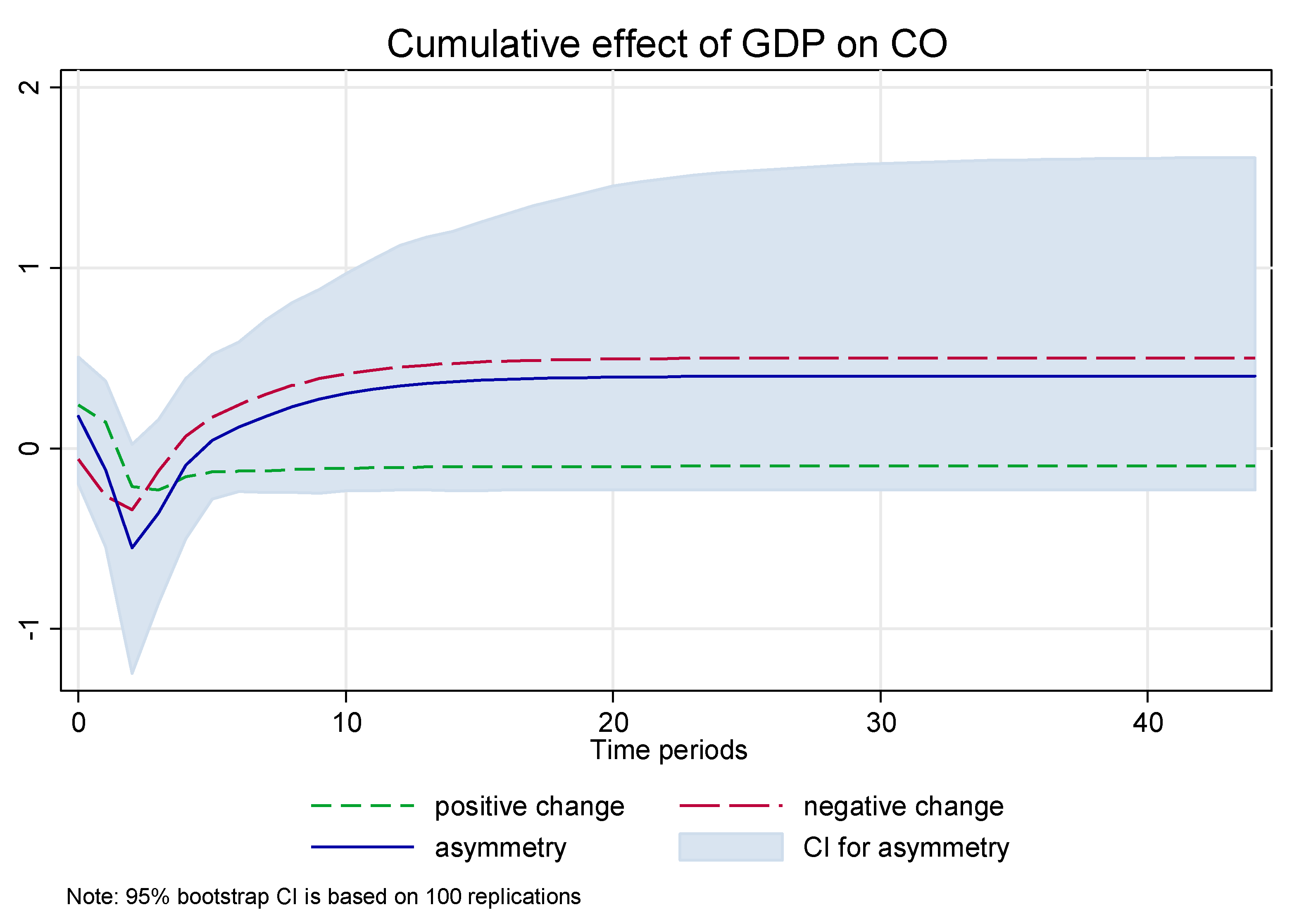
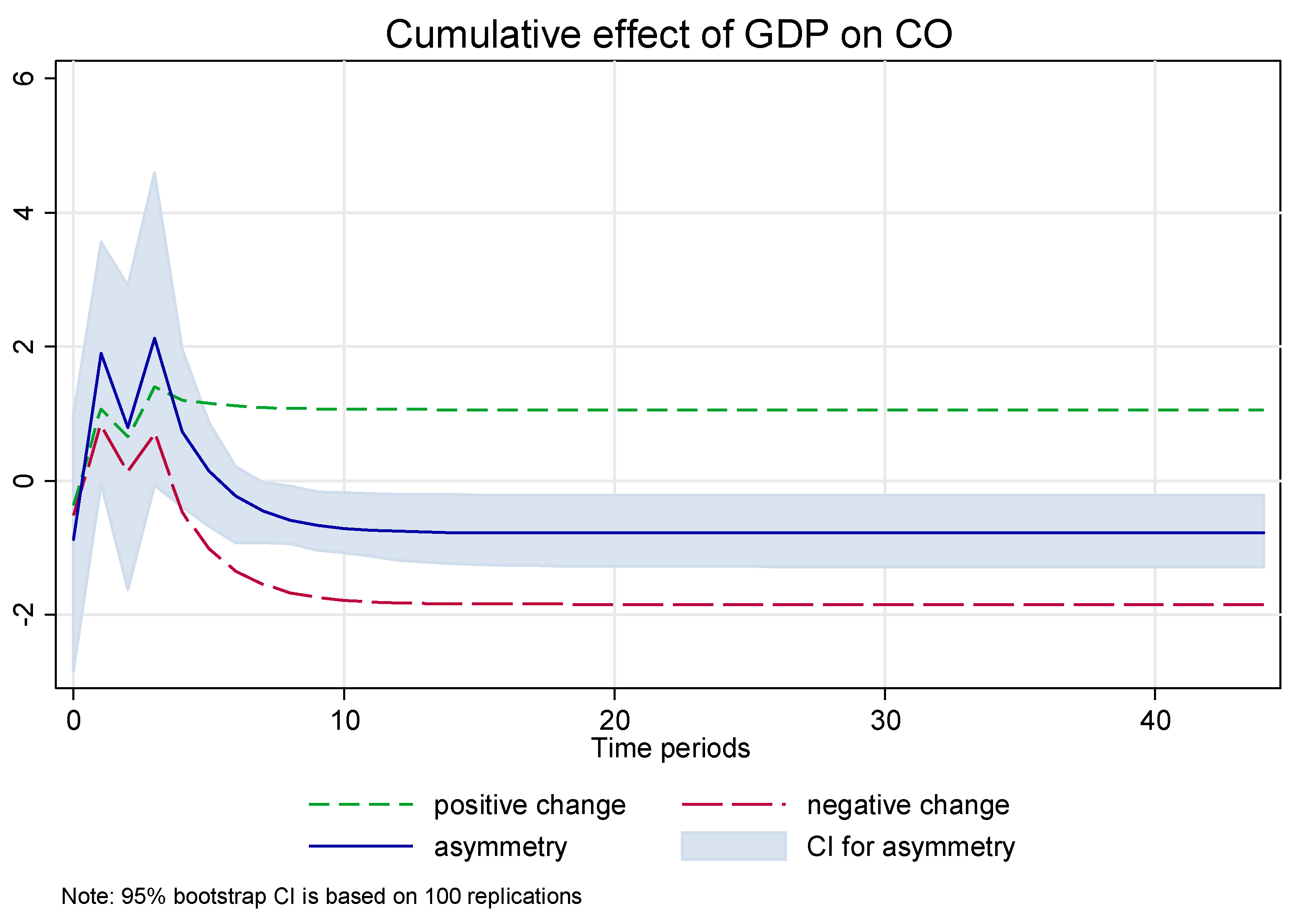
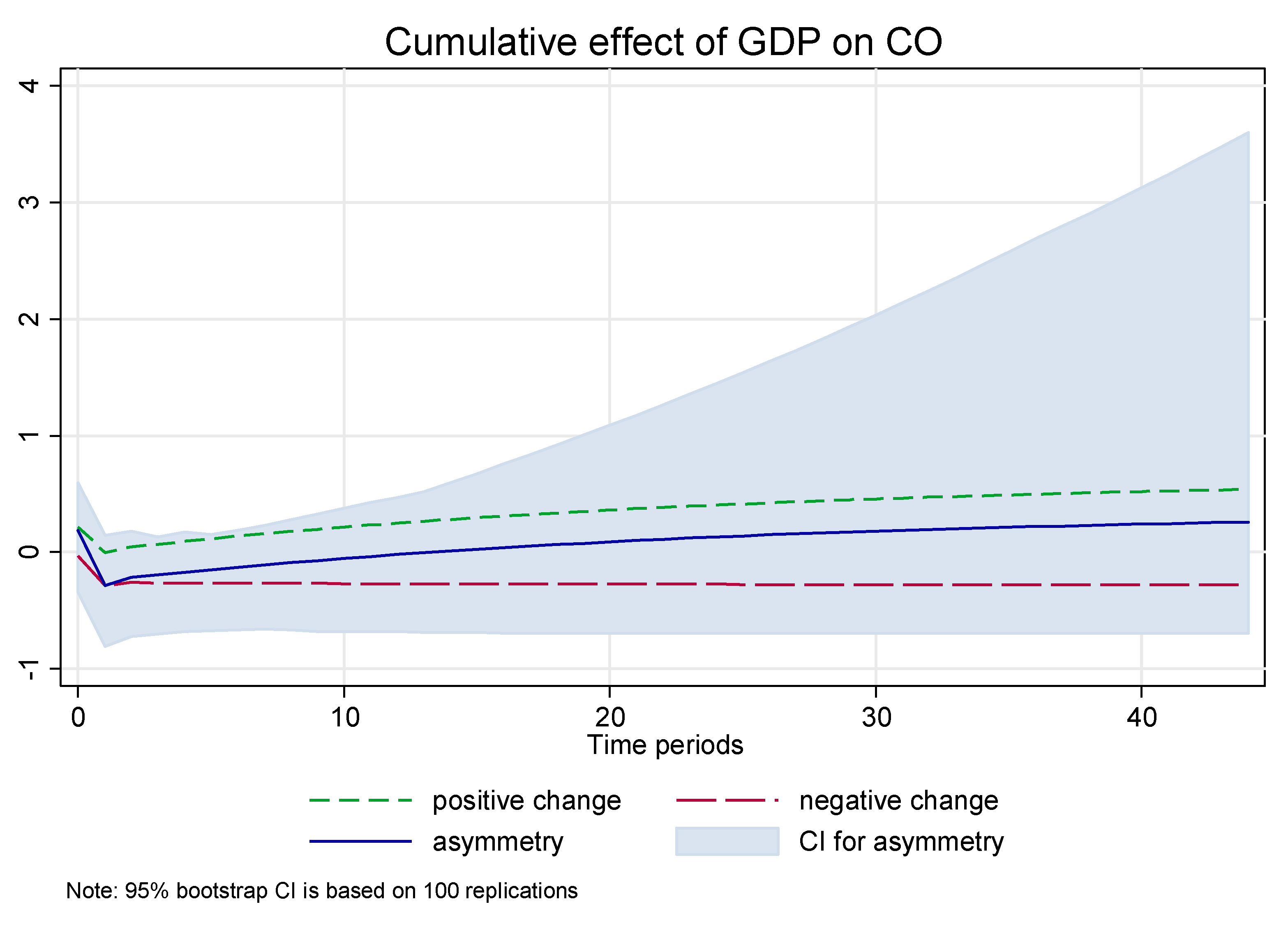
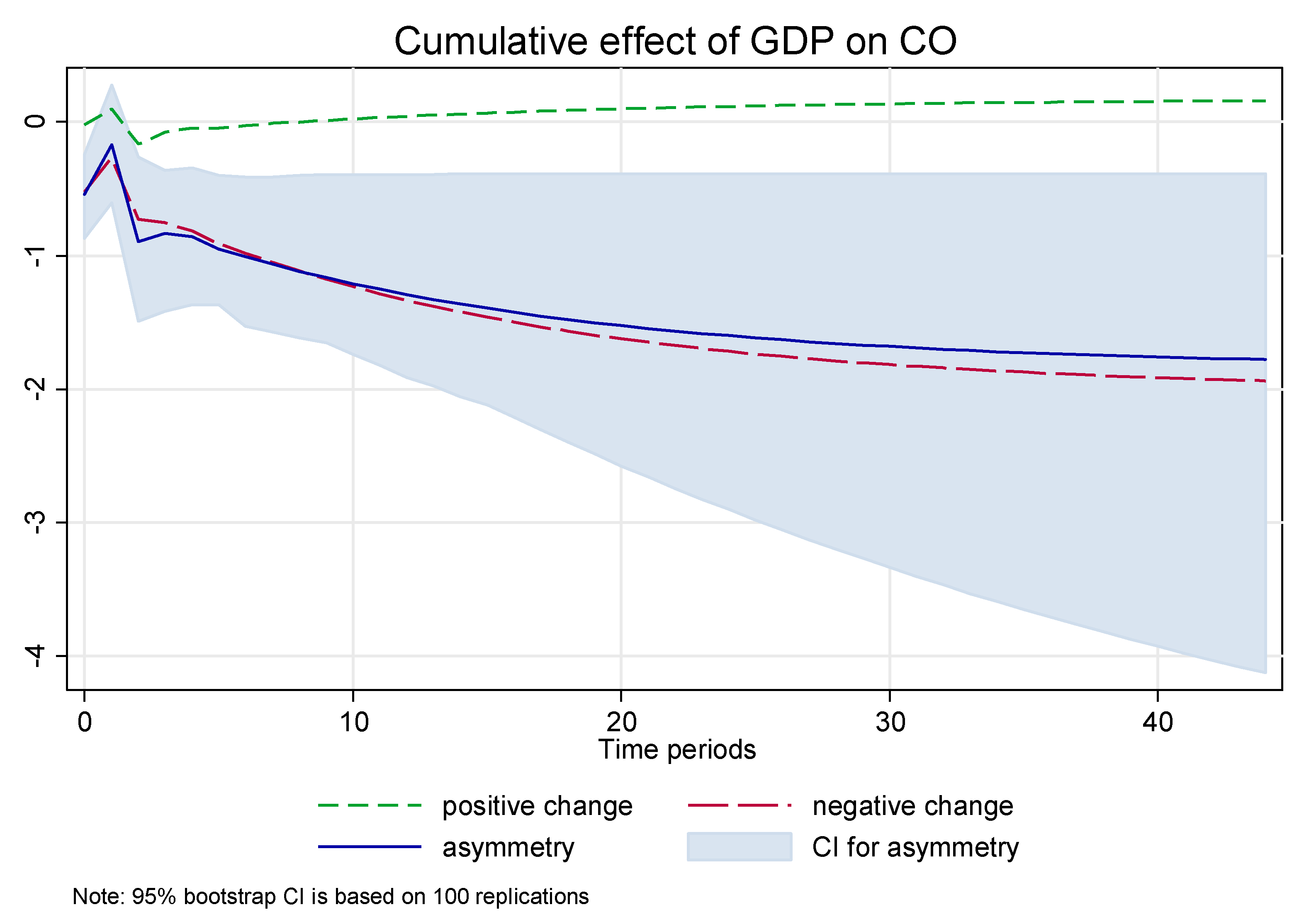
The dynamic asymmetric relationship between the given variables was further enriched by plotting the multipliers effects. These dynamic multipliers (see Figure A1, Figure A2, Figure A3, Figure A4, Figure A5, Figure A6, Figure A7, Figure A8, Figure A9 and Figure A10 in the Appendix A) show the adjustments of energy consumption and economic growth to a unit shock in carbon emission to its new long-run equilibrium following a positive or negative unitary shock in the 44 years. The positive (dashed green line) and negative (dashed red line) change curves describe the adjustment of energy consumption and economic growth to a positive and negative effect of multipliers to shocks in the 44-year carbon emissions at a given forecast horizon. The asymmetry line (continuous blue line) reflects the difference between the positive and negative effects multipliers to shocks in the 44-year energy consumption and economic growth.
3.8. Asymmetric Causality Result
Result of the short- and long-run asymmetric result were proposed by Diks and Panchenko. Table 11 shows the linear Granger causality test between economic growth, electric consumption, and carbon emission.

Table 11.
Nonlinear Granger causality test.
The findings are exciting and slightly different compared with the conventional Granger test results from Table 11. In the Congo Democratic Republic, we observe a bidirectional asymmetric causality relationship that exists between carbon emission and energy consumption. While in the case of the Congo Republic, we find a unidirectional causality running from energy consumption to carbon emission. We can also see that economic growth contributes to increased energy consumption in the Congo Republic. In the case of Kenya, we have a unidirectional nonlinear Granger causality from energy consumption to carbon emission. Subsequently, our result also shows a unidirectional asymmetric causality running from energy consumption to carbon emission in Nigeria. In the Zambian economy, our findings also show that energy consumption Granger causes carbon emission. Additionally, in Italy, we find the unidirectional asymmetric causality running from energy consumption to carbon emission. Based on our analysis, we document that energy consumption Granger causes carbon emissions in Japan. We find the presence of a unidirectional causality relationship from economic growth to carbon emission in Japan. Furthermore, our results in Japan show a unidirectional linear Granger causality running from economic growth to energy consumption. Finally, we also identified a unidirectional nonlinear Granger causality from energy consumption to carbon emissions and economic growth that contributes to increased carbon emission in the UK economy.
4. Discussion
The results presented in the previous section can be used for electricity consumption and economic growth policy analysis across Canada, France, Italy, Japan, UK, USA, India, Algeria, Cameroon, Congo Democratic Republic, Congo Republic, Ghana, Kenya, Nigeria, and Zambia. Furthermore, comparing the results of previous literature and existing studies could assist researchers in understanding whether the asymmetry matters in modelling the consumption–growth–emission nexus.
Results show a nonlinear cointegration between electric consumption, economic growth, and carbon emission in Congo Republic, Zambia, Canada, Cameroon, and the UK at the usual significant levels for these countries.
In terms of the asymmetric and symmetric relationships between variables, the findings are quite diverse. Results from Table 9 and Table 10 show evidence of a long-run asymmetric link between energy consumption, economic growth, and carbon emission in Cameroon and Canada, which is in line with [36,37,38] who found an asymmetric nexus between energy consumption, economic growth, and carbon emission. Additionally, a short-run asymmetric relationship between economic growth and carbon emission in the Congo Republic and the UK was confirmed.
The results from our nonlinear granger causality tend to be volatile across countries. The nonlinear granger causality test in Table 11 shows that there is bidirectional Granger causality from electric consumption to carbon emission in the Congo Democratic Republic. In the Congo Republic, Kenya, Nigeria, Zambia, Italy, Japan, and the UK, electric consumption Granger causes carbon emissions. In Japan and the UK, the results reveal a unidirectional causality running from economic growth to carbon emission consistent with the results of [22] who reported a unidirectional causality between economic growth and carbon emission in Japan. A unidirectional causality is running from economic growth to electric consumption in the Congo Republic and Japan. From our findings, Congo Republic and Japan governments should search for energy exploration policies to sustain economic growth in the long run as energy consumption boosts economic growth. Local and foreign investors are encouraged to adopt green energy while producing more output. Additionally, the unidirectional causality running from economic growth to carbon emission in Japan and UK implies that economic growth is accompanied by carbon emission; this finding is consistent with [39] who report that economic expansion increases carbon emission. This means introducing environmentally friendly policies should be encouraged to reduce carbon emissions. The feedback effect between electricity consumption and carbon emission is an indication that electric consumption in Congo Democratic Republic, Congo Republic, Kenya Nigeria, Zambia, Italy, Japan, and the UK have intensified carbon emission. It confirmed that there is no causal relationship between economic growth and electric consumption, suggesting that energy policies insignificantly affect electric consumption. The neutral effect of economic growth on electric consumption in the Congo Democratic Republic means that the economic plan will not be affected by the electric consumption because economic growth has little or no role to play in enhancing electric consumption. Finally, energy conservation policy implementation to reduce carbon emission cannot hurt economic growth in Algeria, Cameroon, Ghana, Canada, USA, France, and India. These economies have no causality found between electric consumption, economic group, and carbon emission. Therefore, it implies that electric consumption and economic growth have a minimal role to play in increasing CO2 emissions.
5. Conclusions
This paper analyzed the relationship between electric consumption, economic growth, and carbon emission for 15 countries. The empirical results are mixed across countries. To examine the short-run and long-run relationships between electric consumption, economic growth, and carbon emission over the period 1971-2014, the nonlinear ARDL model procedure proposed by [29] and the asymmetric causality approach developed by [27] were used to this end. Results from the NARDL bounds test estimation confirm the cointegration between electricity consumption, economic growth, and carbon emission in Cameroon, Congo Republic, Zambia, Canada, and the UK. In the case of symmetric and asymmetric causal hypotheses and relationships, the long-run results show the asymmetric relationship between electricity consumption, economic growth, and carbon emission in Cameroon and Canada, while the short-run asymmetric relationship was identified in the Congo Republic and the UK. Therefore, future attempts on this issue should consider the symmetric linkage between the variables and choose an empirical methodology accordingly. This study was limited to 15 countries made up of six of the G7 countries and eight selected African counties in addition to India. Future studies can explore the possible asymmetric relationship between energy consumption, economic growth, and carbon emission in other top global carbon dioxide emitters such as China, Russia, Germany, Iran, and Saudi Arabia.
Author Contributions
Conceptualization, S.L.; methodology, P.C.B., S.L. and Z.W.; software, G.K.M.A.; validation, G.K.M.A. and P.C.B.; formal analysis, P.C.B.; investigation, P.C.B. and D.A.A.; resources, S.L. and Z.W.; data curation, P.C.B.; writing—original draft preparation, P.C.B. and G.K.M.A.; writing—review and editing, P.C.B. and G.K.M.A.; visualization, G.K.M.A., P.C.B. and D.A.A.; supervision, S.L.; project administration, S.L.; funding acquisition, S.L. and Z.W. All authors have read and agreed to the published version of the manuscript.
Funding
This research was funded by National Social Science Foundation of China with grant number No.16BJY049. The APC was funded by Special Fund for Basic Scientific Research of Central Colleges, China University of Geosciences (Wuhan) Grant No.CUG170105.
Acknowledgments
This paper was supported by the National Social Science Foundation of China under Grant No.16BJY049, by the Special Fund for Basic Scientific Research of Central Colleges, China University of Geosciences (Wuhan) Grant No.CUG170105.
Conflicts of Interest
The authors declare no conflict of interest.
Appendix A
Cameroon
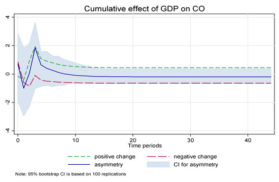
Figure A1.
Cumulative effect of GDP on CO.
Figure A1.
Cumulative effect of GDP on CO.

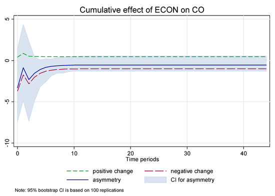
Figure A2.
Cumulative effect of ECON on CO.
Figure A2.
Cumulative effect of ECON on CO.

Canada
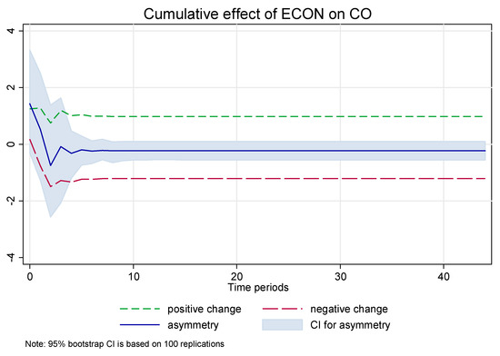
Figure A3.
Cumulative effect of ECON on CO.
Figure A3.
Cumulative effect of ECON on CO.
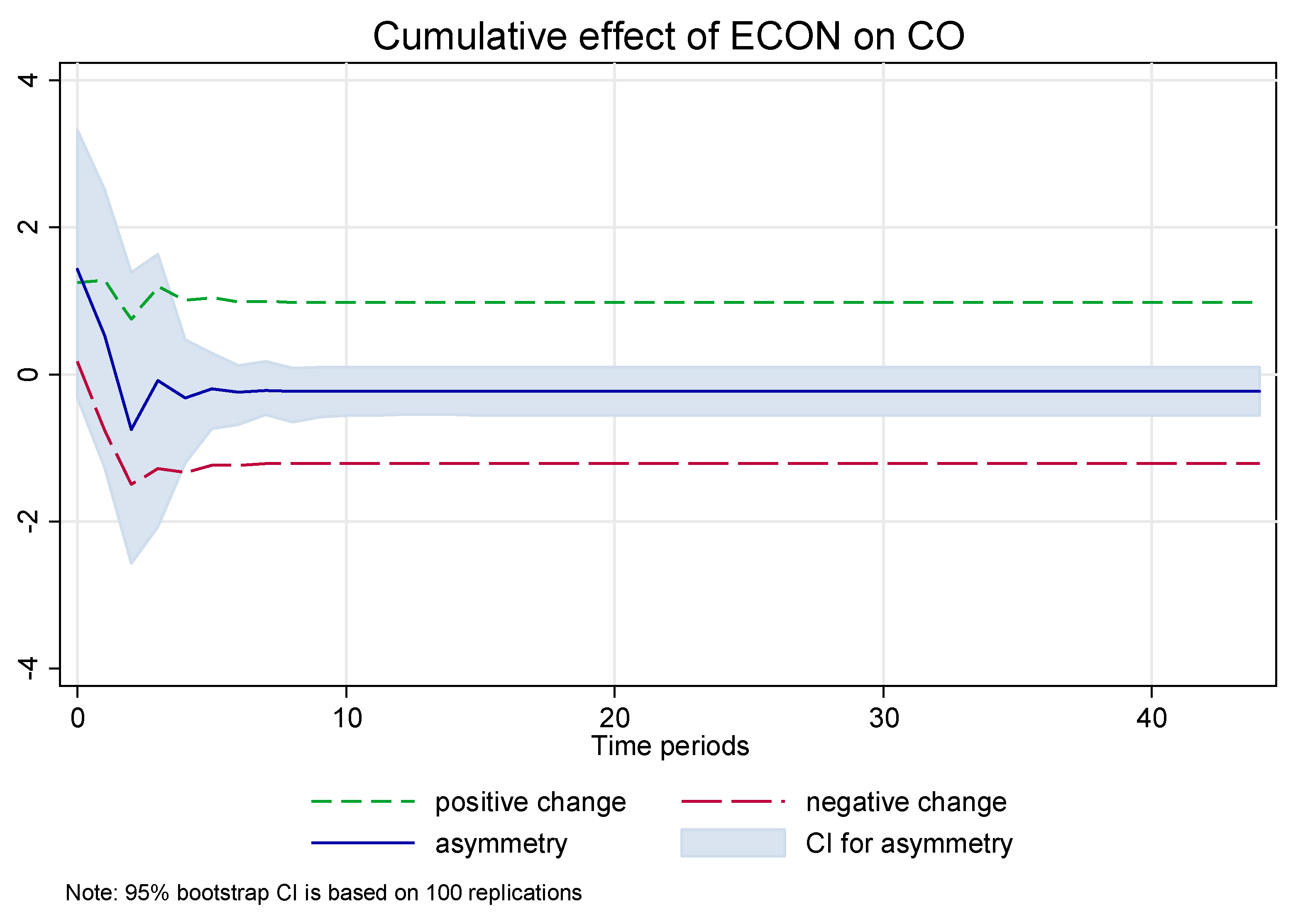
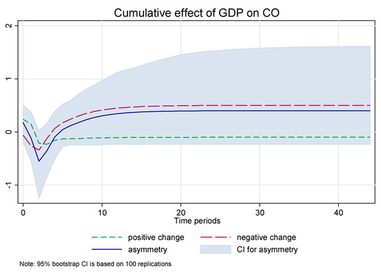
Figure A4.
Cumulative effect of GDP on CO.
Figure A4.
Cumulative effect of GDP on CO.
Congo Republic
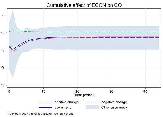
Figure A5.
Cumulative effect of ECON on CO.
Figure A5.
Cumulative effect of ECON on CO.
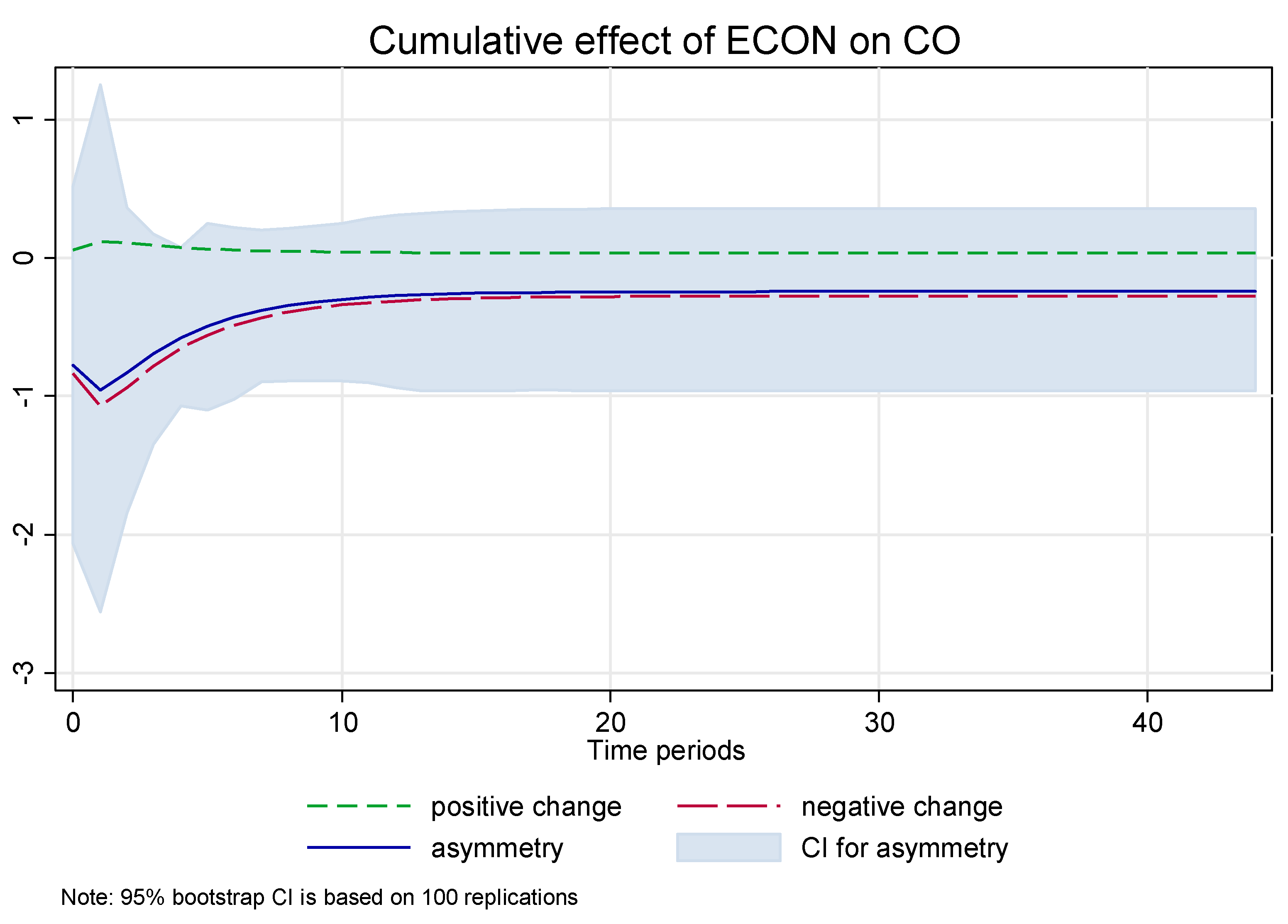
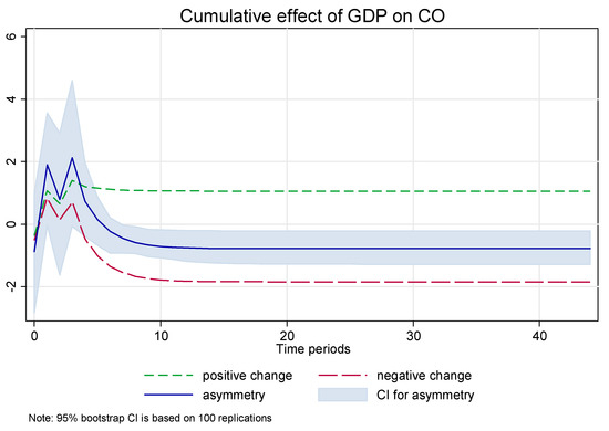
Figure A6.
Cumulative effect of GDP on CO.
Figure A6.
Cumulative effect of GDP on CO.
Zambia
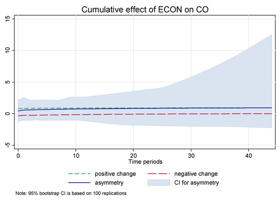
Figure A7.
Cumulative effect of ECON on CO.
Figure A7.
Cumulative effect of ECON on CO.
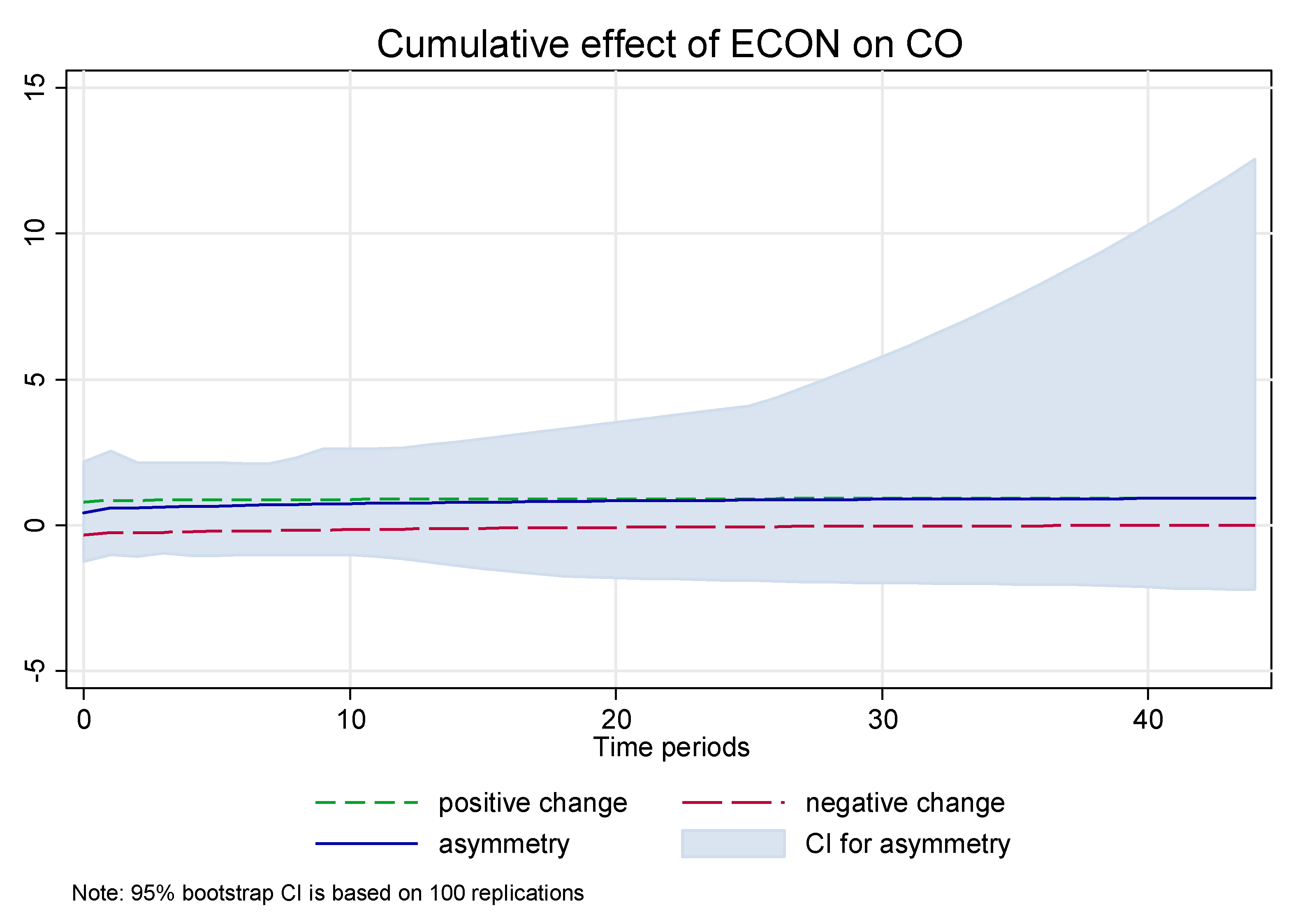
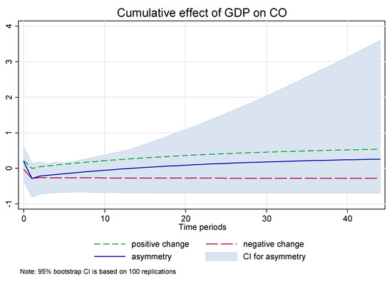
Figure A8.
Cumulative effect of GDP on CO.
Figure A8.
Cumulative effect of GDP on CO.
UK

Figure A9.
Cumulative effect of ECON on CO.
Figure A9.
Cumulative effect of ECON on CO.
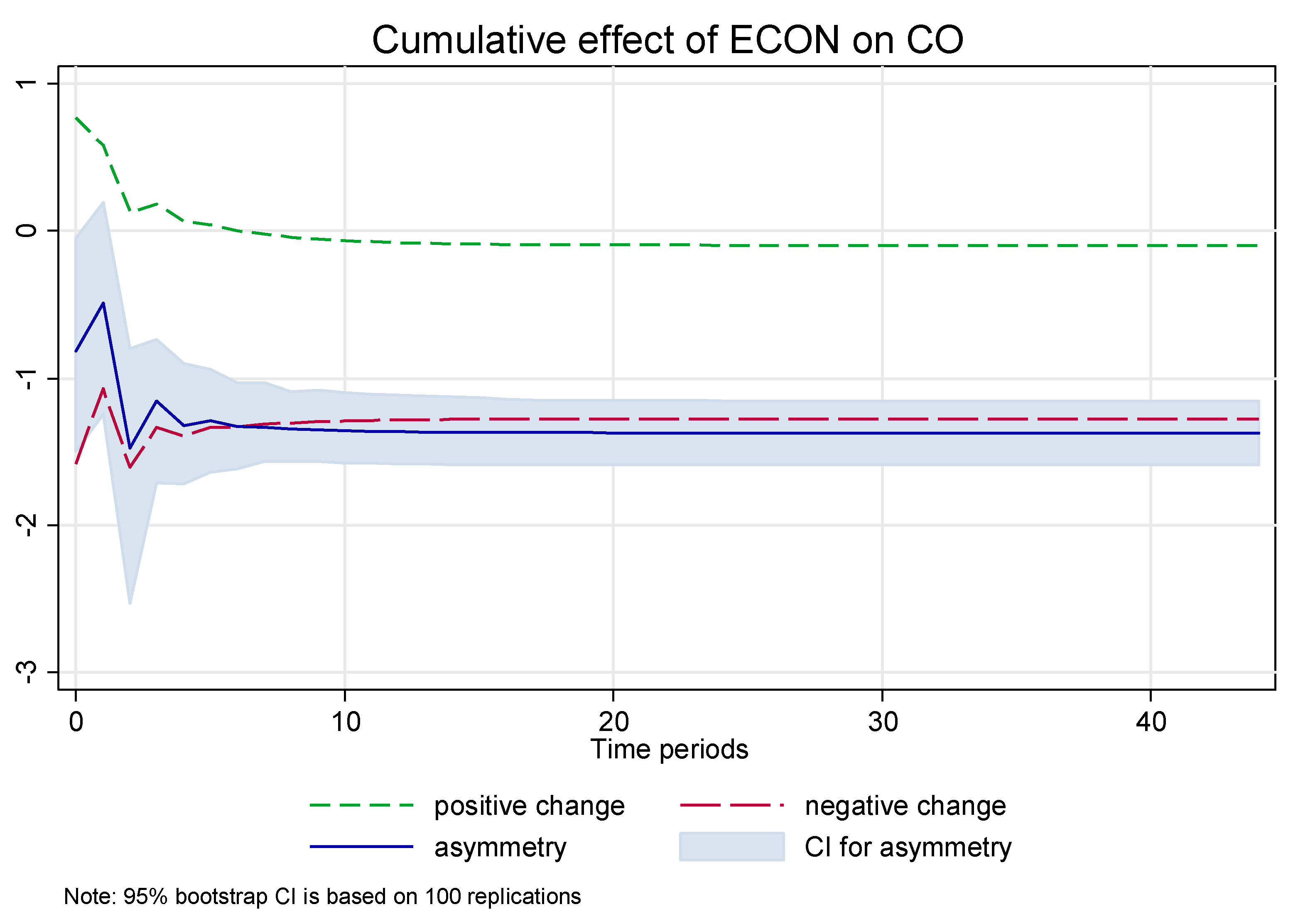

Figure A10.
Cumulative effect of GDP on CO.
Figure A10.
Cumulative effect of GDP on CO.
References
- Ang, J.B. CO2 emissions, energy consumption, and output in France. Energy Policy 2007, 35, 4772–4778. [Google Scholar] [CrossRef]
- Saidi, K.; Hammami, S. The impact of CO2 emissions and economic growth on energy consumption in 58 countries. Energy Rep. 2015, 1, 62–70. [Google Scholar] [CrossRef]
- Hamilton, T.G.A.; Kelly, S. Low carbon energy scenarios for sub-Saharan Africa: An input-output analysis on the effects of universal energy access and economic growth. Energy Policy 2017, 105, 303–319. [Google Scholar] [CrossRef]
- Appiah, K.; Du, J.; Musah, A.; Afriyie, S. Investigation of the relationship between economic growth and carbon dioxide (CO2) emissions as economic structure changes: Evidence from Ghana. Resour. Environ. 2017, 7, 160–167. [Google Scholar]
- Bouznit, M.; Pablo-Romero, M.d.P. CO2 emission and economic growth in Algeria. Energy Policy 2016, 96, 93–104. [Google Scholar] [CrossRef]
- Esso, J.; Keho, Y. Energy consumption, economic growth and carbon emissions: Cointegration and causality evidence from selected African countries. Energy 2016, 114, 492–497. [Google Scholar] [CrossRef]
- Mezghani, I.; Ben Haddad, H. Energy consumption and economic growth: An empirical study of the electricity consumption in Saudi Arabia. Renew. Sustain. Energy Rev. 2017, 75, 145–156. [Google Scholar] [CrossRef]
- Ahmad, A.; Zhao, Y.; Shahbaz, M.; Bano, S.; Zhang, Z.; Wang, S.; Liu, Y. Carbon emissions, energy consumption and economic growth: An aggregate and disaggregate analysis of the Indian economy. Energy Policy 2016, 96, 131–143. [Google Scholar] [CrossRef]
- Gao, J.; Zhang, L. Electricity Consumption–Economic Growth–CO2 Emissions Nexus in Sub-Saharan Africa: Evidence from Panel Cointegration. Afr. Dev. Rev. 2014, 26, 359–371. [Google Scholar] [CrossRef]
- Cowan, W.N.; Chang, T.; Inglesi-Lotz, R.; Gupta, R. The nexus of electricity consumption, economic growth and CO2 emissions in the BRICS countries. Energy Policy 2014, 66, 359–368. [Google Scholar] [CrossRef]
- Lean, H.H.; Smyth, R. CO2 emissions, electricity consumption and output in ASEAN. Appl. Energy 2010, 87, 1858–1864. [Google Scholar] [CrossRef]
- Akpan, G.; Akpan, U. Electricity Consumption, Carbon Emissions and Economic Growth in Nigeria. Int. J. Energy Econ. Policy 2012, 2, 292–306. [Google Scholar]
- Asumadu-Sarkodie, S.; Owusu, P. The relationship between carbon dioxide emissions, electricity production and consumption in Ghana. Energy Sources Part B Econ. Plan. Policy 2017. [Google Scholar] [CrossRef]
- Ajmi, A.N.; Hammoudeh, S.; Nguyen, D.K.; Sato, J.R. On the relationships between CO2 emissions, energy consumption and income: The importance of time variation. Energy Econ. 2015, 49, 629–638. [Google Scholar] [CrossRef]
- Farhani, S.; Rejeb, J.B. Energy consumption, economic growth and CO2 emissions: Evidence from panel data for MENA region. Int. J. Energy Econ. Policy 2012, 2, 71–81. [Google Scholar]
- Ssali, M.W.; Du, J.; Hongo, D.O.; Mensah, I.A. Impact of Economic Growth, Energy Use and Population Growth on Carbon Emissions in Sub-Sahara Africa. J. Environ. Sci. Eng. 2018, 7, 178–192. [Google Scholar]
- Njoke, M.; Wu, Z.; Tamba, J.G. International Journal of Energy Economics and Policy Empirical Analysis of Electricity Consumption, CO2 Emissions and Economic Growth: Evidence from Cameroon. Int. J. Energy Econ. Policy 2019, 9. [Google Scholar] [CrossRef]
- Arango-Miranda, R.; Hausler, R.; Romero-Lopez, R.; Glaus, M.; Ibarra-Zavaleta, S.P. Carbon dioxide emissions, energy consumption and economic growth: A comparative empirical study of selected developed and developing countries.“The role of exergy”. Energies 2018, 11, 2668. [Google Scholar] [CrossRef]
- Riti, J.S.; Song, D.; Shu, Y.; Kamah, M. Decoupling CO2 emission and economic growth in China: Is there consistency in estimation results in analyzing environmental Kuznets curve? J. Clean. Prod. 2017, 166, 1448–1461. [Google Scholar] [CrossRef]
- Chen, P.Y.; Chen, S.T.; Hsu, C.S.; Chen, C.C. Modeling the global relationships among economic growth, energy consumption and CO2 emissions. Renew. Sustain. Energy Rev. 2016, 65, 420–431. [Google Scholar] [CrossRef]
- Ponta, L.; Raberto, M.; Teglio, A.; Cincotti, S. An Agent-based Stock-flow Consistent Model of the Sustainable Transition in the Energy Sector. Ecol. Econ. 2018, 145, 274–300. [Google Scholar] [CrossRef]
- Liu, H.; Lei, M.; Zhang, N.; Du, G. The causal nexus between energy consumption, carbon emissions and economic growth: New evidence from China, India and G7 countries using convergent cross mapping. PLoS ONE 2019, 14, e0217319. [Google Scholar] [CrossRef] [PubMed]
- Karanfil, F. How many times again will we examine the energy-income nexus using a limited range of traditional econometric tools? Energy Policy 2009, 37, 1191–1194. [Google Scholar] [CrossRef]
- Shin, Y.; Yu, B.; Greenwood-Nimmo, M. Modelling asymmetric cointegration and dynamic multipliers in a nonlinear ARDL framework. In Festschrift in Honor of Peter Schmidt; Springer: Berlin/Heidelberg, Germany, 2014; pp. 281–314. [Google Scholar]
- Narayan, P.K.; Narayan, S. Estimating income and price elasticities of imports for Fiji in a cointegration framework. Econ. Model. 2005, 22, 423–438. [Google Scholar] [CrossRef]
- Pesaran, M.H.; Shin, Y.; Smith, R.J. Bounds testing approaches to the analysis of level relationships. J. Appl. Econom. 2001, 16, 289–326. [Google Scholar] [CrossRef]
- Diks, C.; Panchenko, V. A new statistic and practical guidelines for nonparametric Granger causality testing. J. Econ. Dyn. Control 2006, 30, 1647–1669. [Google Scholar] [CrossRef]
- Hiemstra, C.; Jones, J.D. Testing for linear and nonlinear Granger causality in the stock price-volume relation. J. Financ. 1994, 49, 1639–1664. [Google Scholar]
- Shin, Y.; Yu, B.; Greenwood-Nimmo, M. Modelling Asymmetric Cointegration and Dynamic Multipliers in a Nonlinear ARDL Framework; Springer: New York, NY, USA, 2013. [Google Scholar]
- Kisswani, K.M. Evaluating the GDP–energy consumption nexus for the ASEAN-5 countries using nonlinear ARDL model. OPEC Energy Rev. 2017, 41, 318–343. [Google Scholar] [CrossRef]
- Banerjee, A.; Dolado, J.; Mestre, R. Error-correction Mechanism Tests for Cointegration in a Single-equation Framework. J. Time Ser. Anal. 1998, 19, 267–283. [Google Scholar] [CrossRef]
- Dickey, D.A.; Fuller, W.A. Likelihood ratio statistics for autoregressive time series with a unit root. Econom. J. Econom. Soc. 1981, 49, 1057–1072. [Google Scholar] [CrossRef]
- Phillips, P.C.; Perron, P. Testing for a unit root in time series regression. Biometrika 1988, 75, 335–346. [Google Scholar] [CrossRef]
- Broock, W.A.; Scheinkman, J.A.; Dechert, W.D.; LeBaron, B. A test for independence based on the correlation dimension. Econom. Rev. 1996, 15, 197–235. [Google Scholar] [CrossRef]
- Kumar, S. On the nonlinear relation between crude oil and gold. Resour. Policy 2017, 51, 219–224. [Google Scholar] [CrossRef]
- Ndoricimpa, A. Analysis of asymmetries in the nexus among energy use, pollution emissions and real output in South Africa. Energy 2017, 125. [Google Scholar] [CrossRef]
- Araç, A.; Hasanov, M. Asymmetries in the dynamic interrelationship between energy consumption and economic growth: Evidence from Turkey. Energy Econ. 2014, 44, 259–269. [Google Scholar] [CrossRef]
- Hatemi, J.A.; Uddin, G.S. Is the causal nexus of energy utilization and economic growth asymmetric in the US? Econ. Syst. 2012, 36, 461–469. [Google Scholar] [CrossRef]
- Ridzuan, A.R.; Razak, M.; Mohammad, N.J.; Fatimah, N.; Abdul Latiff, A.R. Nexus among Carbon Emissions, Real Output and Energy Consumption in Malaysia and South Korea: New Evidence using Non-Linear Autoregressive Distributed Lag (NARDL) Analysis. J. Ekon. Malays. 2018, 52, 39–54. [Google Scholar] [CrossRef]
© 2020 by the authors. Licensee MDPI, Basel, Switzerland. This article is an open access article distributed under the terms and conditions of the Creative Commons Attribution (CC BY) license (http://creativecommons.org/licenses/by/4.0/).
