Assessing the Use of Reinforcement Learning for Integrated Voltage/Frequency Control in AC Microgrids


Abstract
1. Introduction
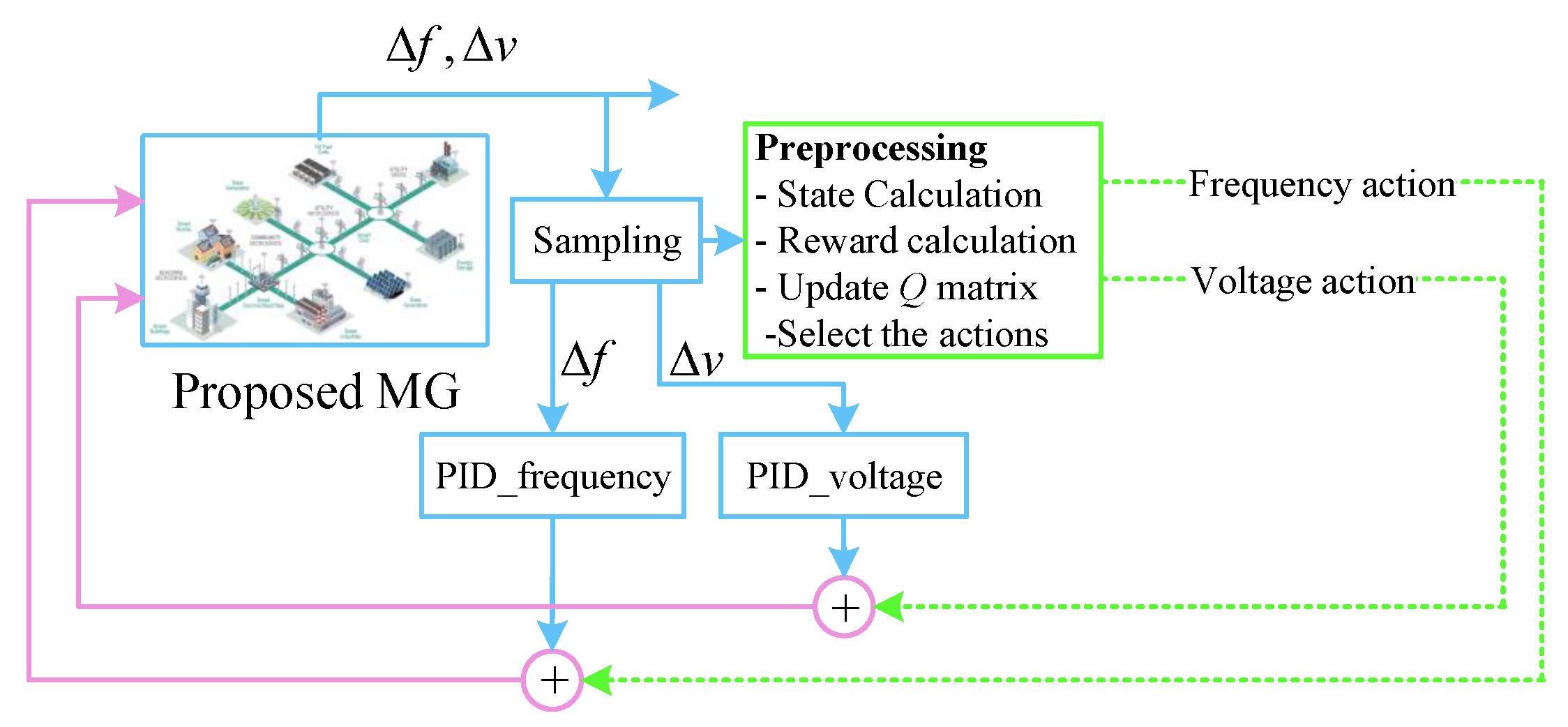
- Modelling the continuous-time environment of MG control as an MDP and solve it using multi-agent reinforcement learning.
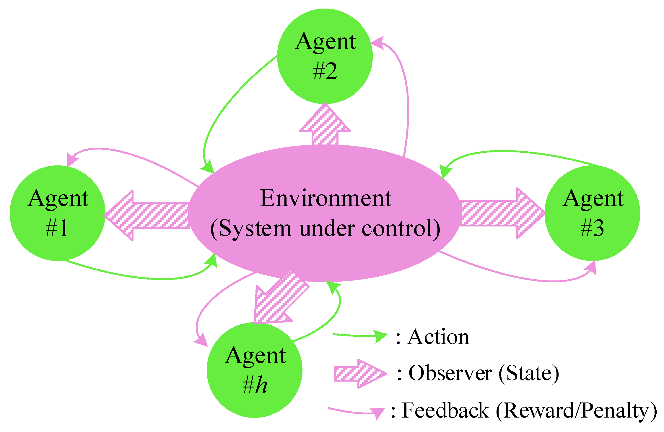
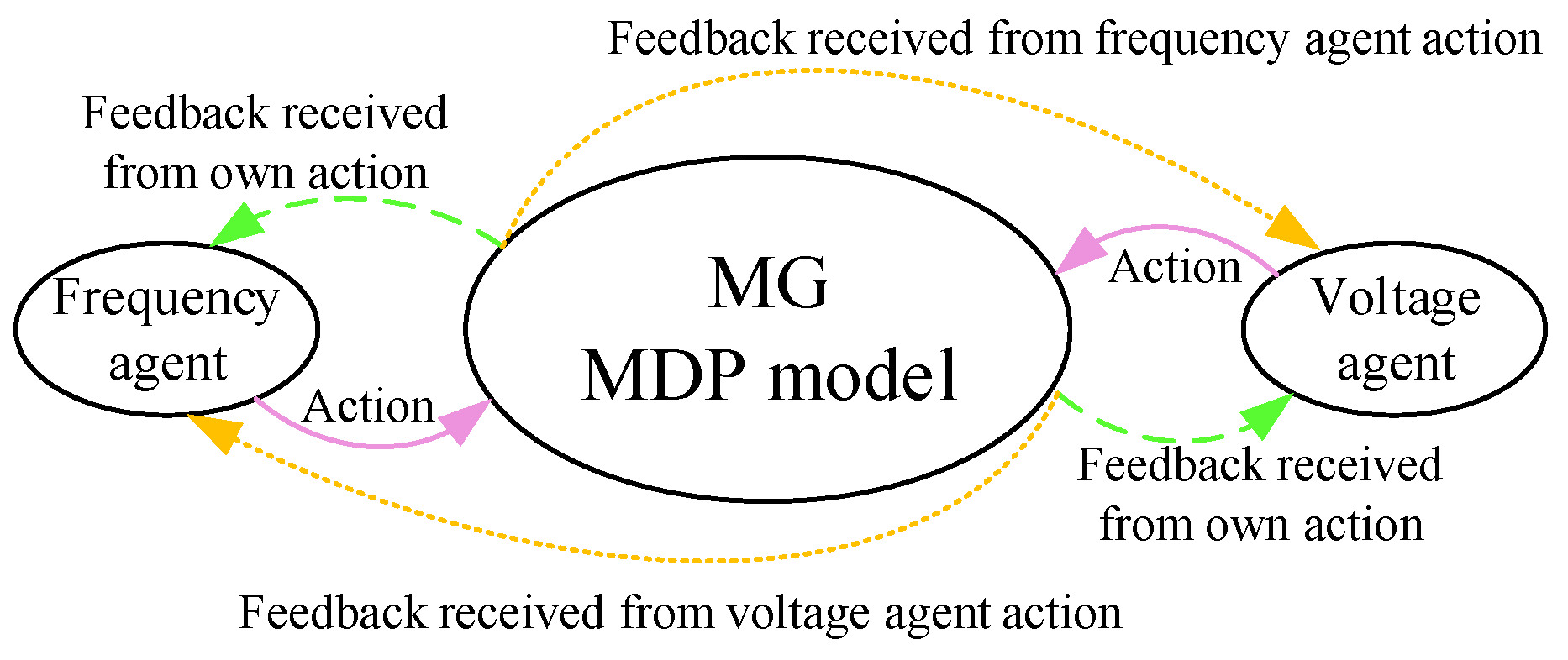
- Considering independent intelligent agents to control the voltage and frequency in order to implement multi-agent reinforcement learning.
- Using model-free Q-learning to cope with system nonlinearities.
- Suggesting a simple strategy to assign the proper instant reward to the voltage and frequency agents according to system dynamics.
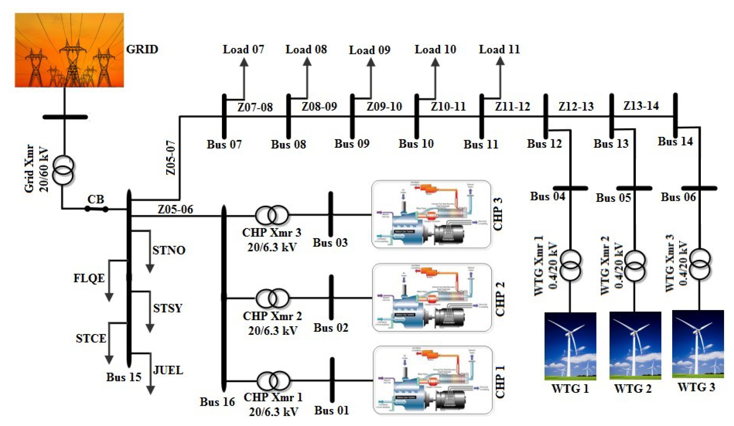
- Employing the nonlinear model of a real microgrid at realistic scenarios for assessing the proposed MDP-based control strategy.
2. Materials and Methods
2.1. The Suggested Game Theory Approach
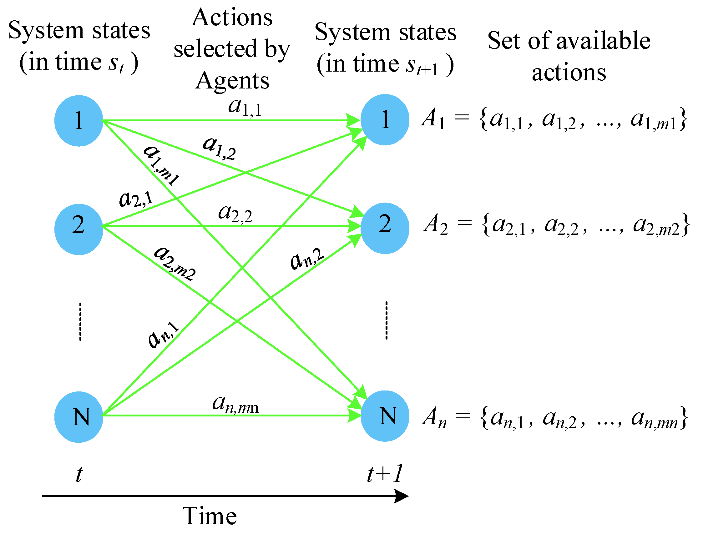
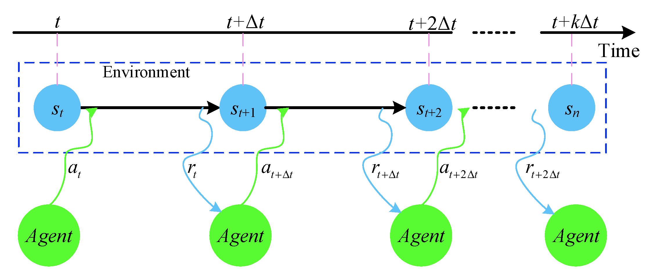
2.1.1. Markov Decision Process
2.1.2. Reinforcement Learning
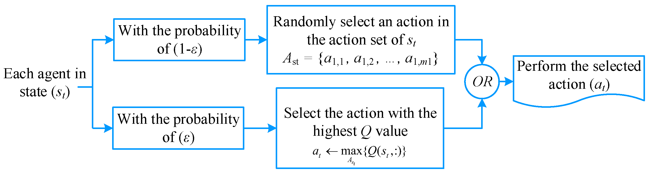
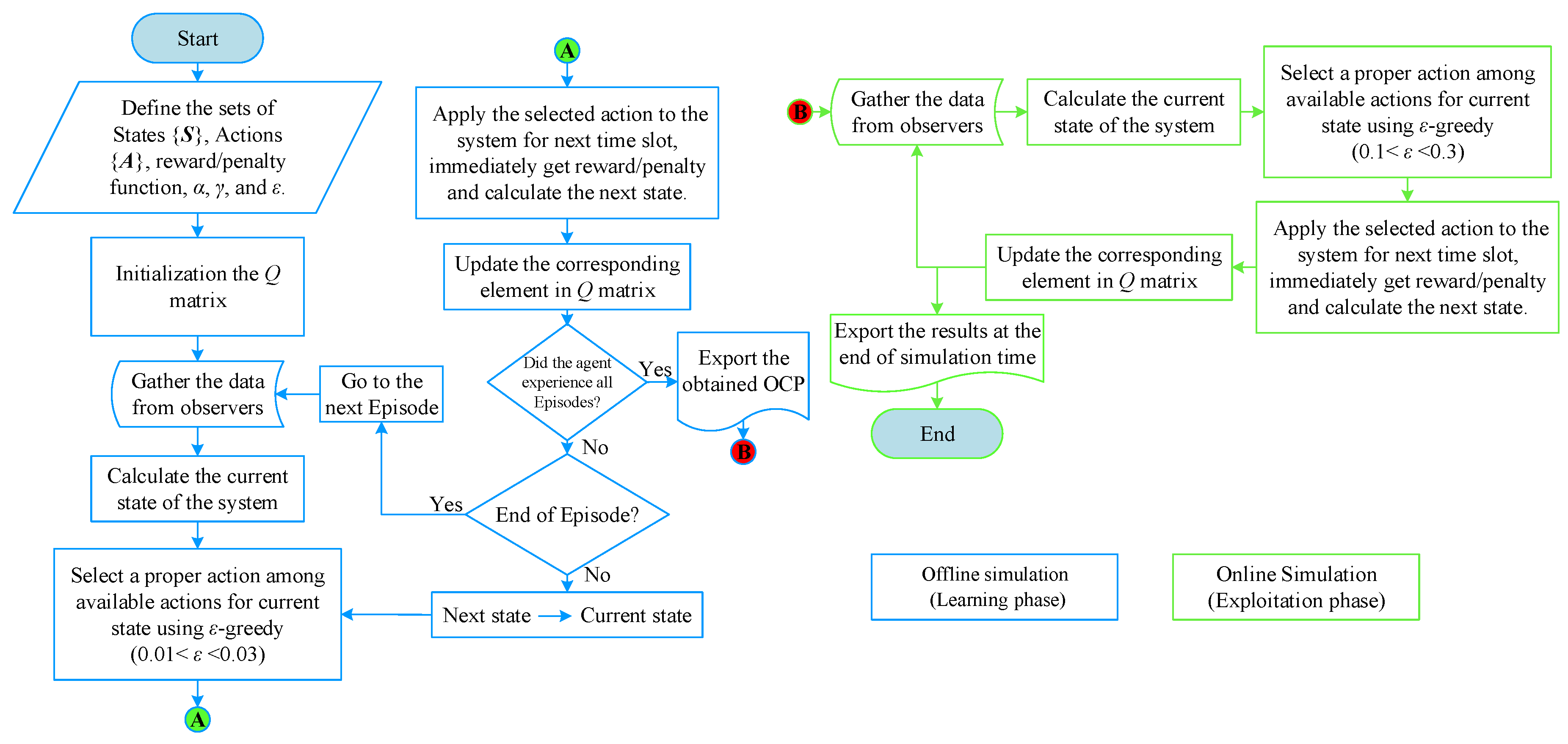
2.1.3. Q-Learning
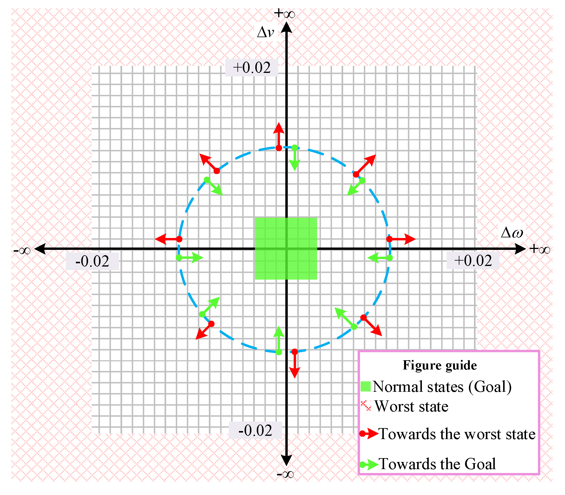
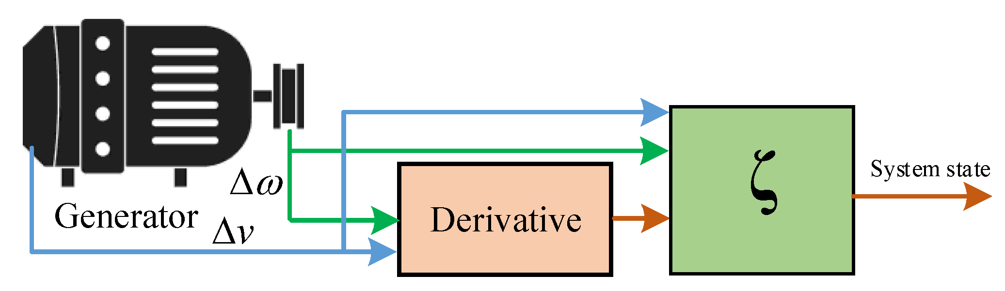
2.1.4. States
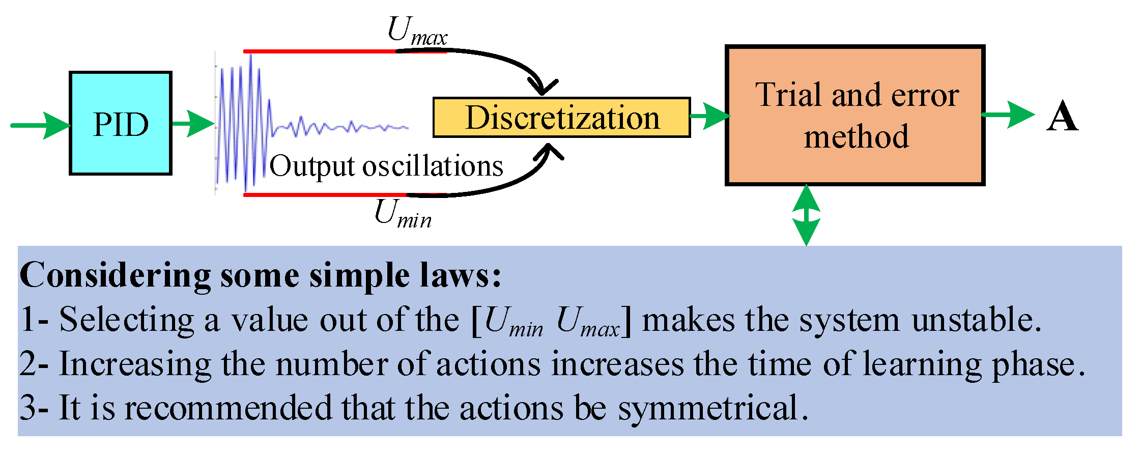
2.1.5. Actions
2.1.6. Reward/Penalty Function
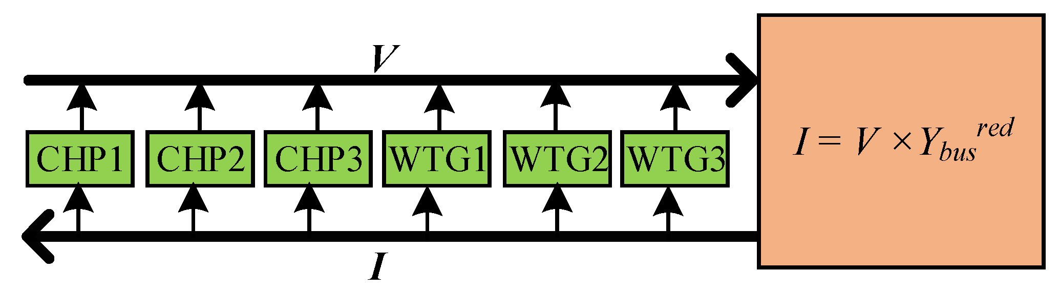
2.2. Dynamic Modelling of the Microgrid Test Case
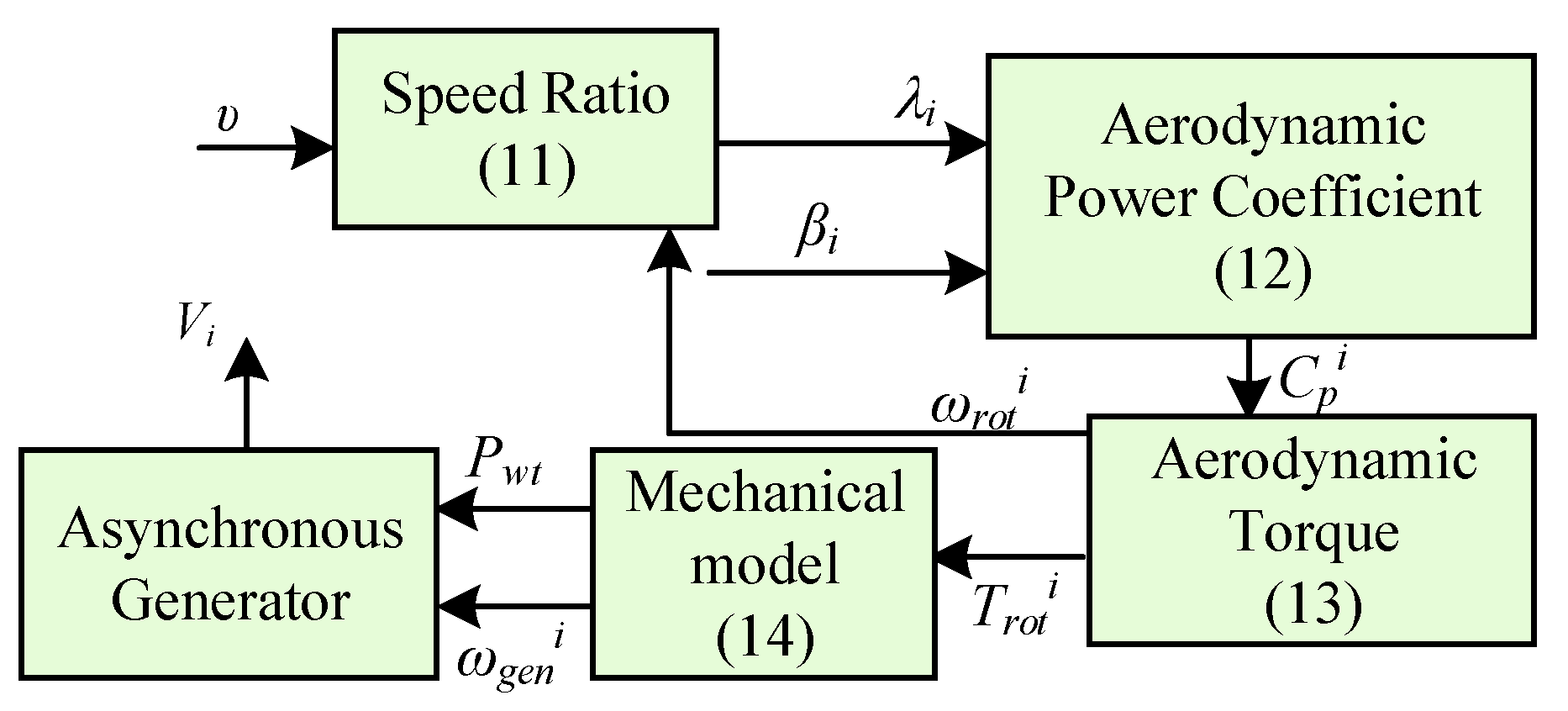
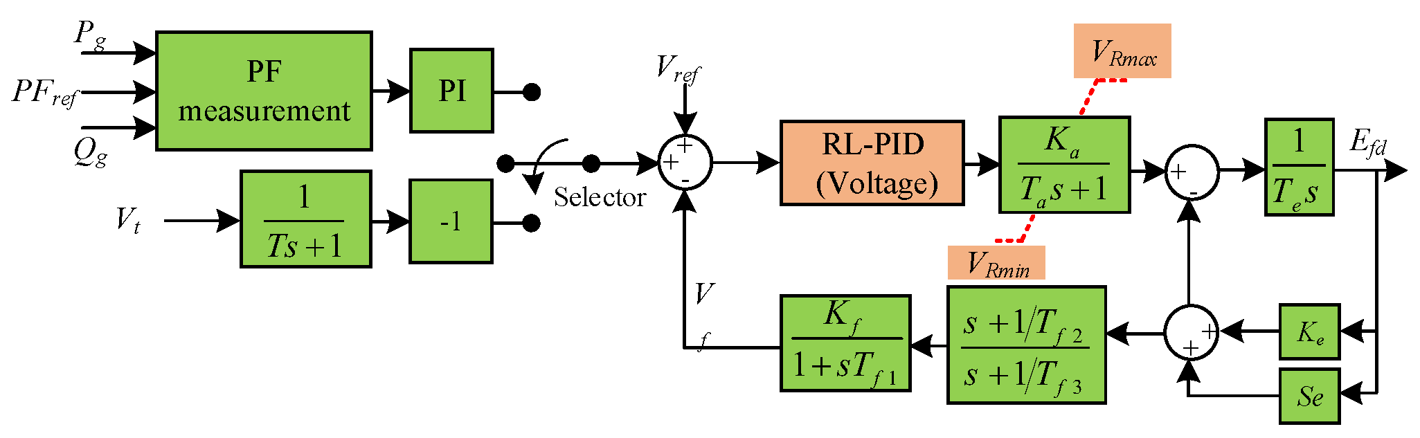
2.2.1. Fixed-Speed Wind Turbine Generator Model
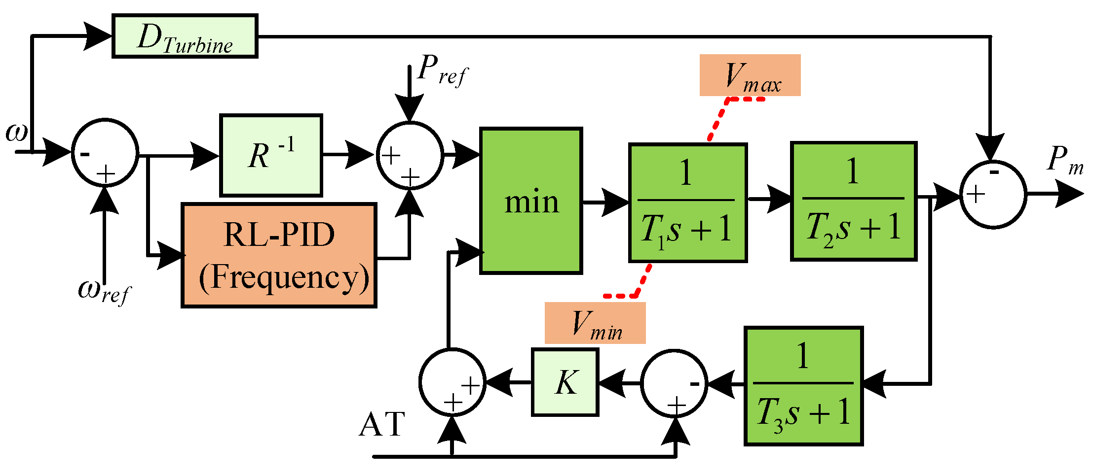
2.2.2. Combined Heat and Power Plant Model
3. Simulation Results
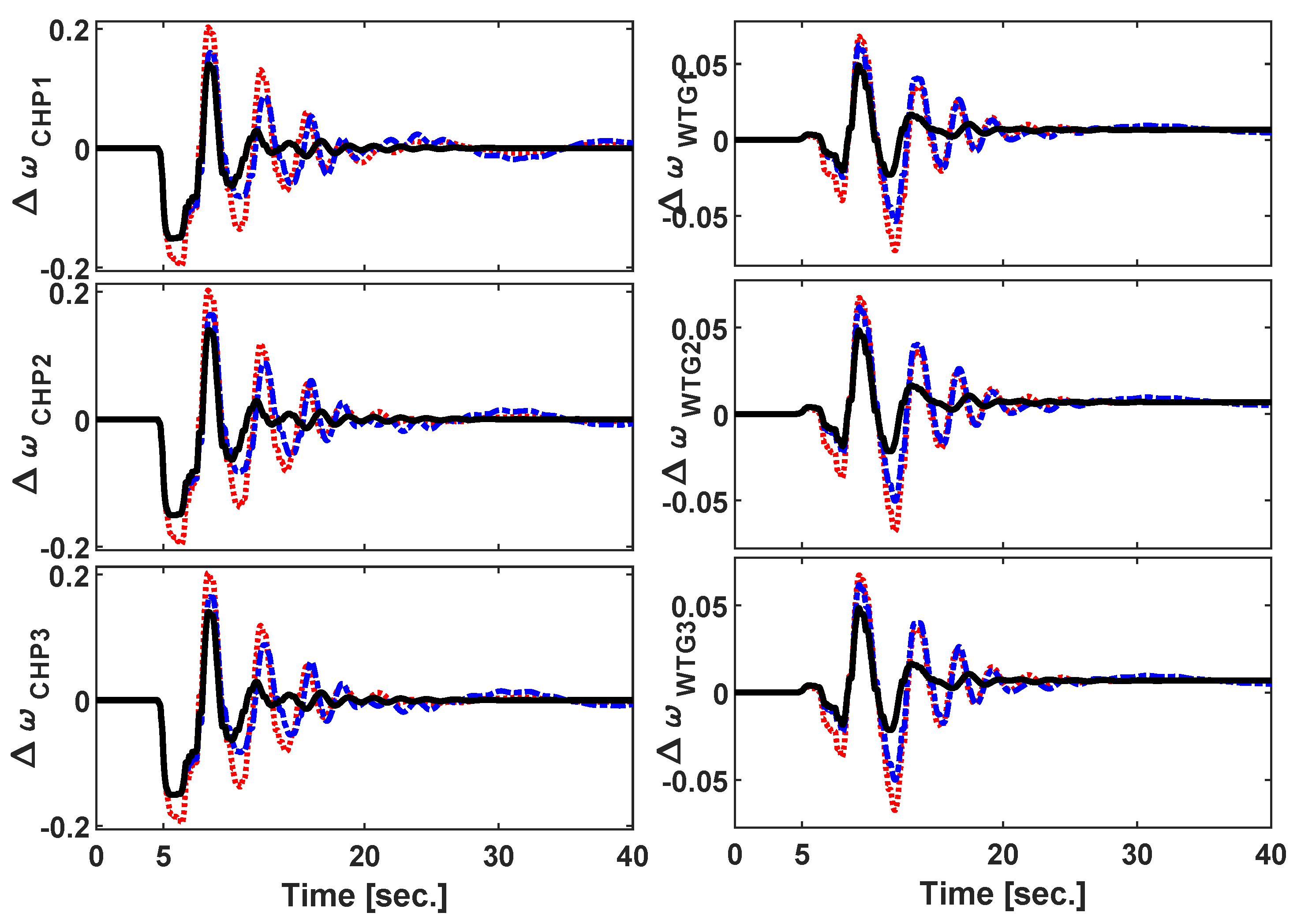
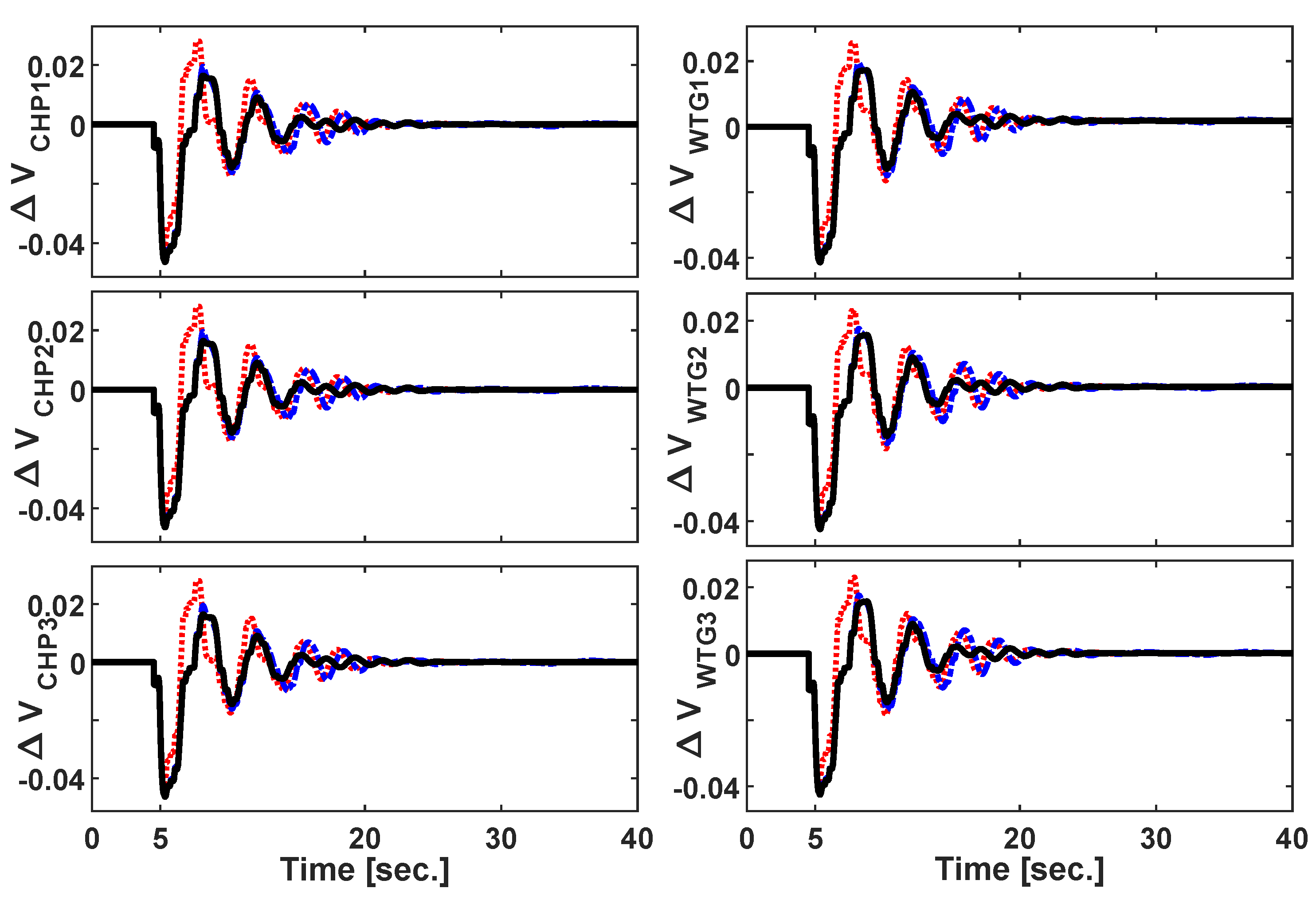
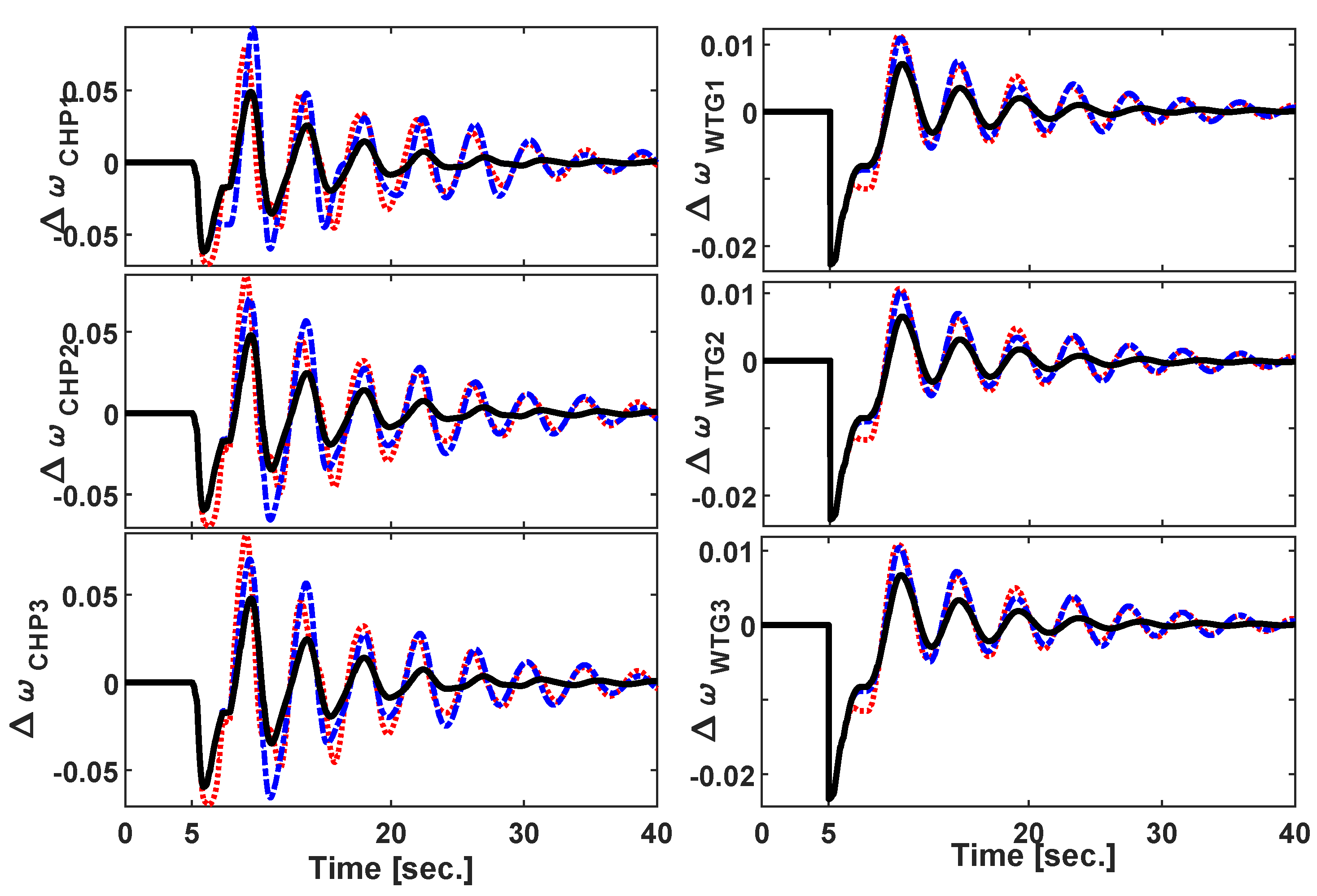
3.1. Scenario 1: Symmetric Three-Phase Fault
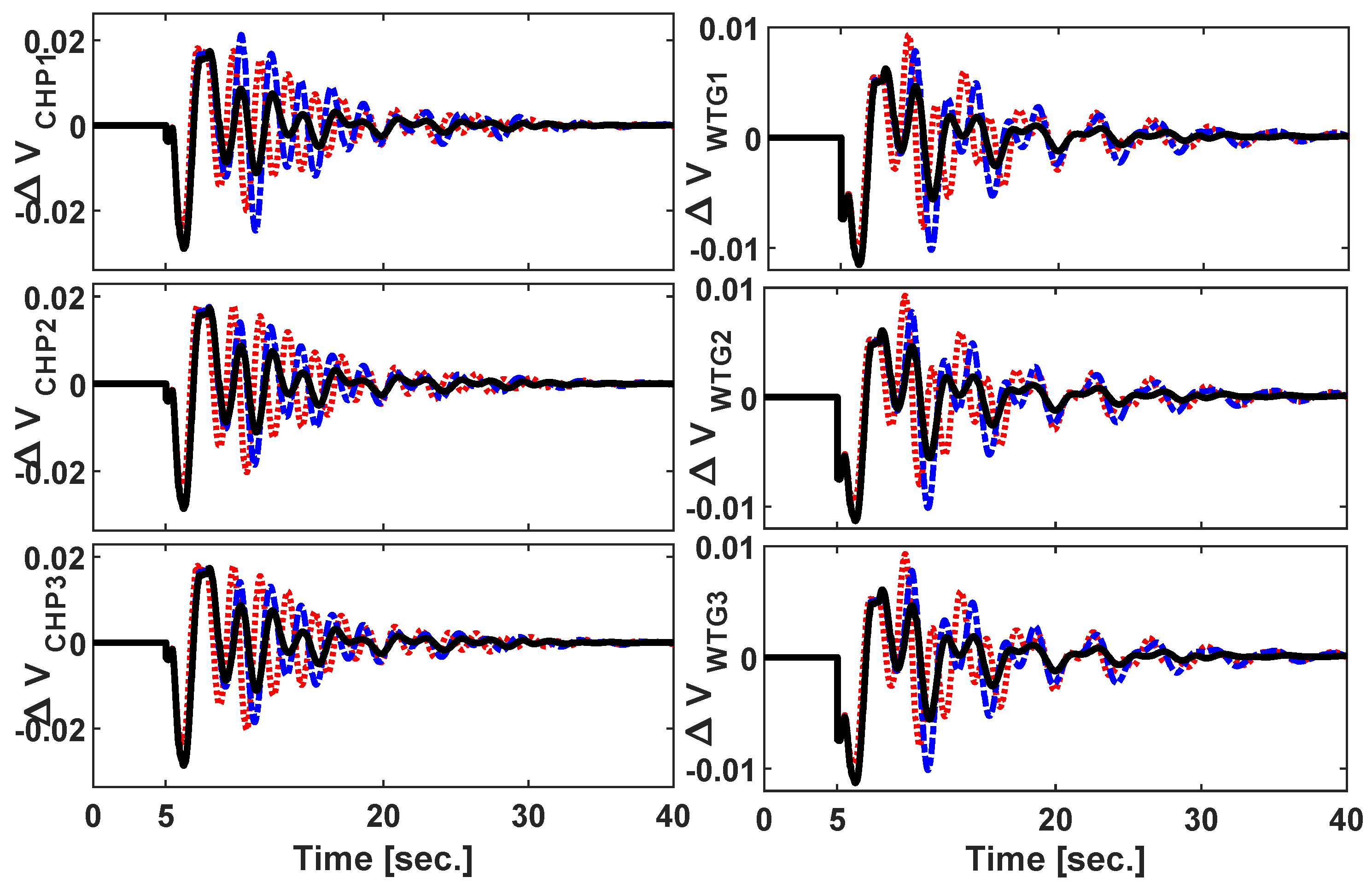
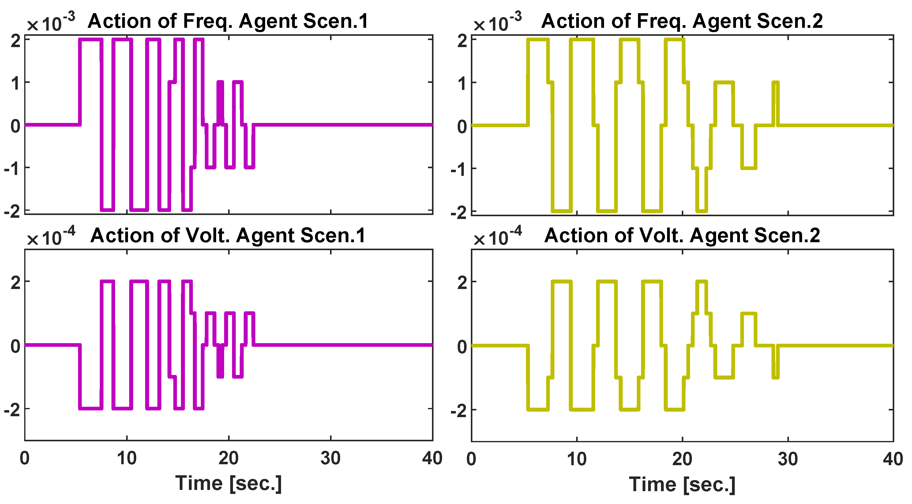
3.2. Scenario 2: Sudden Load Connection/Disconnection
4. Discussion
5. Conclusions
Author Contributions
Funding
Conflicts of Interest
References
- Morshed, M.J.; Fekih, A. A fault-tolerant control paradigm for microgrid-connected wind energy systems. IEEE Syst. J. 2016, 12, 360–372. [Google Scholar] [CrossRef]
- Magdy, G.; Shabib, G.; Elbaset, A.A.; Mitani, Y. A Novel Coordination Scheme of Virtual Inertia Control and Digital Protection for Microgrid Dynamic Security Considering High Renewable Energy Penetration. IET Renew. Power Gener. 2019, 13, 462–474. [Google Scholar] [CrossRef]
- Alam, M.N.; Chakrabarti, S.; Ghosh, A. Networked microgrids: State-of-the-art and future perspectives. IEEE Trans. Ind. Inf. 2018, 15, 1238–1250. [Google Scholar] [CrossRef]
- Gungor, V.C.; Sahin, D.; Kocak, T.; Ergut, S.; Buccella, C.; Cecati, C.; Hancke, G.P. Smart grid technologies: Communication technologies and standards. IEEE Trans. Ind. Inf. 2011, 7, 529–539. [Google Scholar] [CrossRef]
- Ahmed, M.; Meegahapola, L.; Vahidnia, A.; Datta, M. Analysis and mitigation of low-frequency oscillations in hybrid AC/DC microgrids with dynamic loads. IET Gener. Transm. Distrib. 2019, 13, 1477–1488. [Google Scholar] [CrossRef]
- Amoateng, D.O.; Al Hosani, M.; Elmoursi, M.S.; Turitsyn, K.; Kirtley, J.L. Adaptive voltage and frequency control of islanded multi-microgrids. IEEE Trans. Power Syst. 2017, 33, 4454–4465. [Google Scholar] [CrossRef]
- Wu, X.; Shen, C.; Iravani, R. A distributed, cooperative frequency and voltage control for microgrids. IEEE Trans. Smart Grid 2016, 9, 2764–2776. [Google Scholar] [CrossRef]
- De Nadai Nascimento, B.; Zambroni de Souza, A.C.; de Carvalho Costa, J.G.; Castilla, M. Load shedding scheme with under-frequency and undervoltage corrective actions to supply high priority loads in islanded microgrids. IET Renew. Power Gener. 2019, 13, 1981–1989. [Google Scholar] [CrossRef]
- Shrivastava, S.; Subudhi, B.; Das, S. Noise-resilient voltage and frequency synchronisation of an autonomous microgrid. IET Gener. Transm. Distrib. 2019, 13, 189–200. [Google Scholar] [CrossRef]
- Liu, Z.; Miao, S.; Fan, Z.; Liu, J.; Tu, Q. Improved power flow control strategy of the hybrid AC/DC microgrid based on VSM. IET Gener. Transm. Distrib. 2019, 13, 81–91. [Google Scholar] [CrossRef]
- El Tawil, T.; Yao, G.; Charpentier, J.F.; Benbouzid, M. Design and analysis of a virtual synchronous generator control strategy in microgrid application for stand-alone sites. IET Gener. Transm. Distrib. 2019, 13, 2154–2161. [Google Scholar] [CrossRef]
- Hirase, Y.; Abe, K.; Sugimoto, K.; Sakimoto, K.; Bevrani, H.; Ise, T. A novel control approach for virtual synchronous generators to suppress frequency and voltage fluctuations in microgrids. Appl. Energy 2018, 210, 699–710. [Google Scholar] [CrossRef]
- La Gatta, P.O.; Passos Filho, J.A.; Pereira, J.L.R. Tools for handling steady-state under-frequency regulation in isolated microgrids. IET Renew. Power Gener. 2019, 13, 609–617. [Google Scholar] [CrossRef]
- Simpson-Porco, J.W.; Dörfler, F.; Bullo, F. Voltage stabilization in microgrids via quadratic droop control. IEEE Trans. Autom. Control 2016, 62, 1239–1253. [Google Scholar] [CrossRef]
- Gao, F.; Bozhko, S.; Costabeber, A.; Patel, C.; Wheeler, P.; Hill, C.I.; Asher, G. Comparative stability analysis of droop control approaches in voltage-source-converter-based DC microgrids. IEEE Trans. Power Electron. 2016, 32, 2395–2415. [Google Scholar] [CrossRef]
- Asghar, F.; Talha, M.; Kim, S. Robust frequency and voltage stability control strategy for standalone AC/DC hybrid microgrid. Energies 2017, 10, 760. [Google Scholar] [CrossRef]
- Hosseinalizadeh, T.; Kebriaei, H.; Salmasi, F.R. Decentralised robust T-S fuzzy controller for a parallel islanded AC microgrid. IET Gener. Transm. Distrib. 2019, 13, 1589–1598. [Google Scholar] [CrossRef]
- Zhao, H.; Hong, M.; Lin, W.; Loparo, K.A. Voltage and frequency regulation of microgrid with battery energy storage systems. IEEE Trans. Smart Grid 2017, 10, 414–424. [Google Scholar] [CrossRef]
- Ahmarinejad, A.; Falahjoo, B.; Babaei, M. The stability control of micro-grid after islanding caused by error. Energy Procedia 2017, 141, 587–593. [Google Scholar] [CrossRef]
- Issa, W.; Sharkh, S.M.; Albadwawi, R.; Abusara, M.; Mallick, T.K. DC link voltage control during sudden load changes in AC microgrids. In Proceedings of the 2017 IEEE 26th International Symposium on Industrial Electronics (ISIE), Edinburgh, UK, 19–21 June 2017; pp. 76–81. [Google Scholar]
- Firdaus, A.; Mishra, S. Auxiliary signal-assisted droop-based secondary frequency control of inverter-based PV microgrids for improvement in power sharing and system stability. IET Renew. Power Gener. 2019, 13, 2328–2337. [Google Scholar] [CrossRef]
- Susto, G.A.; Schirru, A.; Pampuri, S.; McLoone, S.; Beghi, A. Machine learning for predictive maintenance: A multiple classifier approach. IEEE Trans. Ind. Inf. 2014, 11, 812–820. [Google Scholar] [CrossRef]
- Elsherif, F.; Chong, E.K.P.; Kim, J. Energy-Efficient Base Station Control Framework for 5G Cellular Networks Based on Markov Decision Process. IEEE Trans. Veh. Technol. 2019, 68, 9267–9279. [Google Scholar] [CrossRef]
- Ernst, D.; Glavic, M.; Wehenkel, L. Power systems stability control: Reinforcement learning framework. IEEE Trans. Power Syst. 2004, 19, 427–435. [Google Scholar] [CrossRef]
- Shayeghi, H.; Younesi, A. Adaptive and Online Control of Microgrids Using Multi-agent Reinforcement Learning. In Microgrid Architectures, Control and Protection Methods; Mahdavi Tabatabaei, N., Kabalci, E., Bizon, N., Eds.; Springer International Publishing: Cham, Switzerland, 2020; pp. 577–602. [Google Scholar]
- Younesi, A.; Shayeghi, H.A. Q-Learning Based Supervisory PID Controller for Damping Frequency Oscillations in a Hybrid Mini/Micro-Grid. Iran. J. Electr. Electron. Eng. 2019, 15. [Google Scholar] [CrossRef]
- Yu, T.; Zhen, W.G. A reinforcement learning approach to power system stabilizer. In Proceedings of the 2009 IEEE Power & Energy Society General Meeting, Calgary, AB, Canada, 26–30 July 2009; pp. 1–5. [Google Scholar]
- Vlachogiannis, J.G.; Hatziargyriou, N.D. Reinforcement learning for reactive power control. IEEE Trans. Power Syst. 2004, 19, 1317–1325. [Google Scholar] [CrossRef]
- Nanduri, V.; Das, T.K. A reinforcement learning model to assess market power under auction-based energy pricing. IEEE Trans. Power Syst. 2007, 22, 85–95. [Google Scholar] [CrossRef]
- Younesi, A.; Shayeghi, H.; Moradzadeh, M. Application of reinforcement learning for generating optimal control signal to the IPFC for damping of low-frequency oscillations. Int. Trans. Electr. Energy Syst. 2018, 28, e2488. [Google Scholar] [CrossRef]
- Hadidi, R.; Jeyasurya, B. Reinforcement learning based real-time wide-area stabilizing control agents to enhance power system stability. IEEE Trans. Smart Grid 2013, 4, 489–497. [Google Scholar] [CrossRef]
- Meng, L.; Sanseverino, E.R.; Luna, A.; Dragicevic, T.; Vasquez, J.C.; Guerrero, J.M. Microgrid supervisory controllers and energy management systems: A literature review. Renew. Sustain. Energy Rev. 2016, 60, 1263–1273. [Google Scholar] [CrossRef]
- Bobyr, M.V.; Emelyanov, S.G. A nonlinear method of learning neuro-fuzzy models for dynamic control systems. Appl. Soft Comput. 2020, 88, 106030. [Google Scholar] [CrossRef]
- Craven, M.P.; Curtis, K.M.; Hayes-Gill, B.H.; Thursfield, C. A hybrid neural network/rule-based technique for on-line gesture and hand-written character recognition. In Proceedings of the Fourth IEEE International Conference on Electronics, Circuits and Systems, Cairo, Egypt, 15–18 December 2020. [Google Scholar]
- Gudyś, A.; Sikora, M.; Wróbel, Ł. RuleKit: A comprehensive suite for rule-based learning. Knowl.-Based Syst. 2020, 105480. [Google Scholar] [CrossRef]
- Jafari, M.; Malekjamshidi, Z. Optimal energy management of a residential-based hybrid renewable energy system using rule-based real-time control and 2D dynamic programming optimization method. Renew. Energy 2020, 146, 254–266. [Google Scholar] [CrossRef]
- Das, P.; Choudhary, R.; Sanyal, A. Review Report on Multi-Agent System Control Analysis for Smart Grid System; SSRN 3517356; SSRN: Rochester, NY, USA, 2020. [Google Scholar]
- Salgueiro, Y.; Rivera, M.; Nápoles, G. Multi-agent-Based Decision Support Systems in Smart Microgrids. In Intelligent Decision Technologies 2019; Springer: London, UK, 2020; pp. 123–132. [Google Scholar]
- Shi, H.; Li, X.; Hwang, K.S.; Pan, W.; Xu, G. Decoupled visual servoing with fuzzyQ-learning. IEEE Trans. Ind. Inf. 2016, 14, 241–252. [Google Scholar] [CrossRef]
- Lu, R.; Hong, S.H.; Yu, M. Demand Response for Home Energy Management Using Reinforcement Learning and Artificial Neural Network. IEEE Trans. Smart Grid 2019, 10, 6629–6639. [Google Scholar] [CrossRef]
- Ruan, A.; Shi, A.; Qin, L.; Xu, S.; Zhao, Y. A Reinforcement Learning Based Markov-Decision Process (MDP) Implementation for SRAM FPGAs. IEEE Trans. Circuits Syst. II: Express Briefs 2019. [Google Scholar] [CrossRef]
- Wu, J.; Fang, B.; Fang, J.; Chen, X.; Chi, K.T. Sequential topology recovery of complex power systems based on reinforcement learning. Phys. A: Stat. Mech. Its Appl. 2019, 535, 122487. [Google Scholar] [CrossRef]
- Busoniu, L.; Babuska, R.; De Schutter, B.; Ernst, D. Reinforcement Learning and Dynamic Programming Using Function Approximators; CRC Press: Boca Raton, FL, USA, 2017. [Google Scholar]
- Song, H.; Liu, C.; Lawarree, J.; Dahlgren, R.W. Optimal electricity supply bidding by Markov decision process. IEEE Trans. Power Syst. 2000, 15, 618–624. [Google Scholar] [CrossRef]
- Xiong, R.; Cao, J.; Yu, Q. Reinforcement learning-based real-time power management for hybrid energy storage system in the plug-in hybrid electric vehicle. Appl. Energy 2018, 211, 538–548. [Google Scholar] [CrossRef]
- Weber, C.; Elshaw, M.; Mayer, N.M. Reinforcement Learning; BoD–Books on Demand: Norderstedt, Germany, 2008. [Google Scholar]
- Kaelbling, L.P.; Littman, M.L.; Moore, A.W. Reinforcement learning: A survey. J. Artif. Intell. Res. 1996, 4, 237–285. [Google Scholar] [CrossRef]
- Sutton, R.S.; Barto, A.G. Reinforcement Learning: An Introduction; MIT Press: Cambridge, MA, USA, 2018. [Google Scholar]
- Watkins, C.J.; Dayan, P. Q-learning. Mach. Learn. 1992, 8, 279–292. [Google Scholar] [CrossRef]
- Bellman, R. Dynamic programming. Science 1966, 153, 34–37. [Google Scholar] [CrossRef]
- Ernst, D. Near Optimal Closed-loop Control. Application to Electric Power Systems. Ph.D. Thesis, University of Liège, Liège, Belgium, 2003. [Google Scholar]
- Nowé, A.; Vrancx, P.; De Hauwere, Y.M. Game theory and multi-agent reinforcement learning. In Reinforcement Learning; Springer: London, UK, 2012; pp. 441–470. [Google Scholar]
- Egido, I.; Fernandez-Bernal, F.; Centeno, P.; Rouco, L. Maximum frequency deviation calculation in small isolated power systems. IEEE Trans. Power Syst. 2009, 24, 1731–1738. [Google Scholar] [CrossRef]
- Gupta, P.; Bhatia, R.; Jain, D. Average absolute frequency deviation value based active islanding detection technique. IEEE Trans. Smart Grid 2014, 6, 26–35. [Google Scholar] [CrossRef]
- Shayeghi, H.; Younesi, A. An online q-learning based multi-agent LFC for a multi-area multi-source power system including distributed energy resources. Iran. J. Electr. Electron. Eng. 2017, 13, 385–398. [Google Scholar]
- Mahat, P.; Chen, Z.; Bak-Jensen, B. Control and operation of distributed generation in distribution systems. Electr. Power Syst. Res. 2011, 81, 495–502. [Google Scholar] [CrossRef]
- Saheb-Koussa, D.; Haddadi, M.; Belhamel, M. Modeling and simulation of windgenerator with fixed speed wind turbine under Matlab-Simulink. Energy Procedia 2012, 18, 701–708. [Google Scholar] [CrossRef]
- Mondal, D.; Chakrabarti, A.; Sengupta, A. Power System Small Signal Stability Analysis and Control; Academic Press: Cambridge, MA, USA, 2014. [Google Scholar]
- Shayeghi, H.; Younesi, A.; Hashemi, Y. Optimal design of a robust discrete parallel FP+ FI+ FD controller for the automatic voltage regulator system. Int. J. Electr. Power Energy Syst. 2015, 67, 66–75. [Google Scholar] [CrossRef]
- Mirjalili, S.; Gandomi, A.H.; Mirjalili, S.Z.; Saremi, S.; Faris, H.; Mirjalili, S.M. Salp Swarm Algorithm: A bio-inspired optimizer for engineering design problems. Adv. Eng. Softw. 2017, 114, 163–191. [Google Scholar] [CrossRef]


| Control Type | F-PID Control | |||||
| Param. | ||||||
| Value | 0.8812 | 1.8235 | 1.6520 | 0.9512 | ||
| Param. | ||||||
| Value | 0.0758 | 1.4510 | 1.3851 | 0.0851 | ||
| Control Type | PID Control | |||||
| Param. | ||||||
| Value | 0.4978 | 0.1408 | 0.00117 | 0.0704 | 0.0383 | 0.0012 |
| Signal | ITAE | ISE | ||||
|---|---|---|---|---|---|---|
| PID | FPID | RLPID | PID | FPID | RLPID | |
| 81.687 | 80.602 | 50.0690 | 2.143 | 1.949 | 1.783 | |
| 78.603 | 76.702 | 50.028 | 2.137 | 1.945 | 1.781 | |
| 78.603 | 76.602 | 50.012 | 2.102 | 1.938 | 1.695 | |
| 62.781 | 60.813 | 54.851 | 1.155 | 1.023 | 0.635 | |
| 62.760 | 60.934 | 54.721 | 1.124 | 1.003 | 0.642 | |
| 62.766 | 60.950 | 54.896 | 1.121 | 1.003 | 0.642 | |
| 13.130 | 10.259 | 2.896 | 0.595 | 0.496 | 0.446 | |
| 3.050 | 10.132 | 2.901 | 0.596 | 0.496 | 0.435 | |
| 13.030 | 10.102 | 2.901 | 0.578 | 0.486 | 0.446 | |
| 27.243 | 26.425 | 5.135 | 0.552 | 0.428 | 0.387 | |
| 14.209 | 11.164 | 5.135 | 0.561 | 0.418 | 0.376 | |
| 13.787 | 10.102 | 3.790 | 0.564 | 0.431 | 0.377 |
| Signal | ITAE | ISE | ||||
|---|---|---|---|---|---|---|
| PID | FPID | RLPID | PID | FPID | RLPID | |
| 4.124 | 4.026 | 3.604 | 2.562 | 2.397 | 1.959 | |
| 4.012 | 4.007 | 3.597 | 2.456 | 2.333 | 1.932 | |
| 4.035 | 4.006 | 3.589 | 2.465 | 2.334 | 1.954 | |
| 3.562 | 3.215 | 2.903 | 1.021 | 0.987 | 0.891 | |
| 3.452 | 3.198 | 2.903 | 1.102 | 0.996 | 0.889 | |
| 3.465 | 3.198 | 2.893 | 1.125 | 0.991 | 0.883 | |
| 3.452 | 3.292 | 2.994 | 1.452 | 1.298 | 1.060 | |
| 3.326 | 3.207 | 2.996 | 1.432 | 1.189 | 1.059 | |
| 3.326 | 3.208 | 2.994 | 1.441 | 1.196 | 1.059 | |
| 3.652 | 2.953 | 2.688 | 0.856 | 0.517 | 0.333 | |
| 3.652 | 2.952 | 2.698 | 0.857 | 0.510 | 0.323 | |
| 3.654 | 2.953 | 2.689 | 0.858 | 0.510 | 0.332 |
© 2020 by the authors. Licensee MDPI, Basel, Switzerland. This article is an open access article distributed under the terms and conditions of the Creative Commons Attribution (CC BY) license (http://creativecommons.org/licenses/by/4.0/).
Share and Cite
Younesi, A.; Shayeghi, H.; Siano, P. Assessing the Use of Reinforcement Learning for Integrated Voltage/Frequency Control in AC Microgrids. Energies 2020, 13, 1250. https://doi.org/10.3390/en13051250
Younesi A, Shayeghi H, Siano P. Assessing the Use of Reinforcement Learning for Integrated Voltage/Frequency Control in AC Microgrids. Energies. 2020; 13(5):1250. https://doi.org/10.3390/en13051250
Chicago/Turabian StyleYounesi, Abdollah, Hossein Shayeghi, and Pierluigi Siano. 2020. "Assessing the Use of Reinforcement Learning for Integrated Voltage/Frequency Control in AC Microgrids" Energies 13, no. 5: 1250. https://doi.org/10.3390/en13051250
APA StyleYounesi, A., Shayeghi, H., & Siano, P. (2020). Assessing the Use of Reinforcement Learning for Integrated Voltage/Frequency Control in AC Microgrids. Energies, 13(5), 1250. https://doi.org/10.3390/en13051250