Abstract
Increasing nonlinearity in today’s grid challenges the conventional small-signal (modal) analysis (SSA) tools. For instance, the interactions among modes, which are not captured by SSA, may play significant roles in a stressed power system. Consequently, alternative nonlinear modal analysis tools, notably Normal Form (NF) and Modal Series (MS) methods are being explored. However, they are computation-intensive due to numerous polynomial coefficients required. This paper proposes a fast NF technique for power system modal interaction investigation, which uses characteristics of system modes to carefully select relevant terms to be considered in the analysis. The Coefficients related to these terms are selectively computed and the resulting approximate model is computationally reduced compared to the one in which all the coefficients are computed. This leads to a very rapid nonlinear modal analysis of the power systems. The reduced model is used to study interactions of modes in a two-area power system where the tested scenarios give same results as the full model, with about 70% reduction in computation time.
1. Introduction
The paradigm shift in power generation does not leave the power system without many challenges. The vast majority of renewable energy (RE) generations and proliferation of electrical vehicle (EV) charging stations lead to complex behaviour of the grid [1]. As highlighted in [2,3], the penetration of RE introduces new oscillations and stability related issues. Moreover, power electronic (PE) converters interfacing these new technologies to the grid also raise some concerns. For example, the PE converters could form a virtual capacitance, which could interact with the AC grid to trigger an unstable subsynchronous oscillation in a relatively weak system [4]. Each type of RE or EV creates challenges ranging from over-voltage, under-voltage, harmonics, stability issues, and many more. Apart from these new challenges, the operation of the grid near its margins, due to some constraints, is not uncommon nowadays. All these lead to a grid which exhibits complex nonlinear behaviour. Consequently, the conventional linear modal analysis tools give deceptive characterisation of the system behaviour [5].
There has been serious research interest on nonlinear tools which would preserve the inferences possible with conventional linear modal analysis. Such inferences include stability assessment, mode-in-state participation factor, system description with concept of modes, and lots more. Mode is the mathematical term for one eigenvalue/eigenvector pair of the linear part of the dynamical system under study. It also refers to the associated particular oscillation pattern and frequency associated to the eigenvector. In the literature, these tools are formulated by including the higher order terms of the Taylor expansion of the system model to obtain an approximate model [6]. They provide better information about the system characteristics than the conventional modal analysis. Prominent among these tools are Normal Form (NF) and Modal Series (MS) techniques. Normal Form uses sequence of nonlinear coordinate transformations to remove the nonlinearities in the approximate Taylor expansion model to obtain a simplified system, easy to analyze [7]. Under certain conditions, a closed-form solution is easily obtained. The resulting simplified systems have many advantages and can be used to extend many linear techniques. For instance, (1) they provide information on nonlinear interactions of modes, which helps to design better controls for power systems; (2) nonlinear mode-in-state participation factors can be defined for better sitting of PSS; (3) modal interaction also gives insights into the stability of the nonlinear system; (4) the nonlinear interaction enables to explain the sources of unknown frequencies appearing in time responses. The authors in [8] used NF to show that modal interactions can have significant effects on the control performance. This aroused interest in the use of NF for control designs. In [9], an approach for control design of the excitation system based on NF was proposed. Various research works show that the nonlinear participation factors analysis possible with NF, could provide more reliable information than the linear one (see for example, [6,10,11]). As a result, better methods for designing [12] and siting [13,14] PSS using NF have been developed. By studying the interactions of modes during disturbance, various stability indices using NF have been proposed in literature (see [5,15,16]). The usefulness of NF analysis triggered further investigation on the effects of second and third order modal interaction on the system dynamics [17,18]. The nonlinear transformation involved in NF leads to a complex representation of the state variables, thereby befuddling its physical meaning. The authors in [18] proposed a method for applying NF, which exploits the sparsity of the power system structure and preserves the physical meaning of the original variables. Real valued NF transformation has also been proposed and used for predicting the stability boundary of the power systems in [19,20]. Reference [21] provides useful guides for validating the NF solutions.
Modal series is similar to NF, only that nonlinear transformation is avoided [22,23], thereby always retaining the physical meaning of the state variables. However, most recent comparison of both methods shows NF to be more accurate and less burdensome under 3rd order consideration [24].
A major setback in the above techniques, however, is the heavy computation arising from the inclusion of higher order terms in the Taylor expansion. Consequently, it is not possible with the present computing technologies to apply NF to large power systems. Thus, the above benefits of NF cannot be fully exploited. To extend the NF application to large power systems and exploit all its benefits, preliminary steps must include solving this computation problem. Inspired by the potentials of NF, Netto et al. [25] proposed a method based on Koopman Mode Decomposition (KMD) which enables the computation of nonlinear participation factor in similar manner as done with NF. However, a comparison of these methods reveals that the computational burden involved in KMD may be same or even more than that of NF [26]. At the same computational level, NF is preferred because of many information it provides which are not apparent in the other methods. In summary, the existing nonlinear alternatives to linear modal analysis are computation-intensive.
Despite the computational challenges, evolution of the grid suggests that NF may be an indispensable tool in future, since the emerging grid will be highly nonlinear with 100% PE [27,28] and beyond the scope of conventional modal analysis. Also, the sources of the new oscillations accompanying PE penetrations have to be unraveled. Therefore, the need for reducing the computation involved in NF application to power system cannot be over emphasized. In dealing with large systems, NF computations may be lessened by first reducing the size of the grid using network reduction techniques such as the ones in [29,30,31]. This however, does not reduce any operation in NF analysis other than the grid size. A method which facilitates the computation of the polynomial coefficients required for NF application has been proposed in [32,33], however, much reduction is still needed as there are still too many terms being considered.
Insights from previous researches strongly suggest that some selected terms can be considered in NF application without serious damage to the analysis. For example, the authors in [6,34] opined that if the interacting modes are accurately determined by higher order spectra (HOS) analysis or prony method, several computations can be restricted to the interacting modes. The implementation of this suggestion for NF does not exist in literature. Moreover, these preliminary works are not in themselves simple since they are sensitive to simulation data considered and prony is also computationally demanding. The authors in [35] suggested that if there is no strong resonance, coupling terms associated with non-conjugate eigenvalues may not have significant contribution to the system nonlinearity in a classical power system. Two challenges however are—(1) a prior knowledge of the significant terms; (2) convenient computational technique to focus on the significant terms. A reduced order NF study was performed in [36] where some interactions were neglected based on their damping rates and nearness to resonance. In order to estimate the NF coefficients relating to these interactions, the time-domain signal is fitted to the needed coefficients in least square (LS) sense, which makes the modal reconstruction fast. The algorithm requires prerequisite time-domain simulation data which determine the accuracy of LS. More data for accuracy increases the computation, which makes the claimed NF reduction unclear. Also, this method hides the actual contribution of each eigenvalue combination which is key in the study of modal interaction.
The main goal of this paper is to reduce the computational burden associated with NF application to power systems, especially when it is applied to understand the significant modal interactions and the accompanying new frequencies. In previous works, an alternative method for computing selectively any desired term rapidly by avoiding the usual Taylor expansion was proposed [32,33,37]. The present paper investigates further reduction of NF computation by considering fewer terms in the nonlinear approximation based on the information provided by the linear analysis. The analysis is then focused only on the considered terms.
2. Normal Form Theory
Consider a power system represented by a general ordinary N-differential equation,
where is the vector of system states and is a real valued vector field assumed smooth. Bold-face mathematical symbols represent vectors/matrices throughout the paper. Power system is usually represented with differential-algebraic equations (DAEs). Since NF operates with differential equations, Equation (1) should be understood as a system of differential equations with the algebraic variables already substituted.
Let (1) be approximated with 3rd order Taylor series around the equilibrium point as
where .
, , and are respectively the Jacobian, 2nd, and 3rd order Hessian matrices. is the i-th state variable which represents the deviation from the equilibrium point. H.O.T stands for higher order terms. Restricting every expansion to order 3, the term H.O.T will be omitted in all subsequent equations for simplicity. The over bar will henceforth be dropped where the meaning is not confusing. Although higher order terms can be considered, the complexity becomes outrageous, so (2) is limited to 3rd order nonlinearity which is a good compromise.
Suppose , , and are respectively eigenvalue, right, and left eigenvectors of , where is diagonalizable, (2) can be put to Jordan form by a linear transformation expressed as
is the element of , , , while and imply -th elements of , and are respectively.
z is the state variable in NF coordinate, and are respectively complex valued quadratic and cubic NF coefficients, determined such that (3) is simplified.
is a residual term from second order transformation and is expressed as [5].
Assuming that in (5) no denominator is , the second and third order terms in (3) can be removed, putting (3) in a decoupled form
with solution given as
In (7), the initial conditions of the variables are computed by solving a system of nonlinear optimisation equations (8), formulated from (4), for given initial conditions .
The algorithm for obtaining the initial condition is presented in Section 2.2. The solution of (2) after back transformation of z is of the form
where
The 2nd and 3rd terms on the right hand side of (9) represent the effects of the modal interactions in addition to the linear modes on the dynamics of state i. , , and indicate the sizes of mode j’s, mode ’s, and mode ’s contributions to the oscillations of state i respectively. Simply put, they are both nonlinear corrections and extra information added to linear analysis.
In a situation where in (5) there are some denominators (so called resonance condition) or (near resonance), not all the nonlinearities can be removed from (3). Under such case (6) is re-written as
where gathers the terms that cannot be removed. With a method proposed in [24], closed-form solution can still be obtained.
2.1. Indices for Modal Interaction
To quantify modal interactions, some indices are defined.
2.1.1. Nonlinearity Indices
The nonlinearity indices , (see [38,39,40]), defined in (11) and (12), estimate the effect of the 2nd and 3rd order nonlinear terms respectively, in the approximate closed form solution. Large values indicate that the higher-order terms are significant or that the difference between modal and NF variables is large, both cases indicating potential for nonlinear interaction.
The index “0” in the above equations indicates initial conditions.
2.1.2. Nonlinear Interaction Indices
2.1.3. Nonlinear Modal Persistence Indices
These indices estimate the extent of dominance of the mode combinations in the system response [6]. They are defined as
where stands for real part of and for time constant of. measures the settling time of the mode combination interacting with mode . Settling time is here defined as the time taken for a response to remain within 2% of the final value and it is approximately 4 time constants. is a measure of the persistence of the modal combination with respect to the dominant mode. High value of indicates that the influence of the modal combination decays faster with respect to the dominant mode and vice versa. A relatively large value of , tend to show a strong modal interaction of long duration for 2nd and 3rd order interactions respectively.
2.2. Normal Form Initial Condition
The initial condition plays a key role since all the indices depend on it. A robust solution technique proposed in [6] for second order NF is extended here for third order NF as follow:
- Define , the initial condition of the power system after disturbance as , where is the post disturbance equilibrium solution and is the system condition at the end of the disturbance.
- Use the eigenvector to obtain the initial condition in Jordan coordinate as .
- To compute
- I.
- Formulate the solution problem as (8).
- II.
- Choose the initial guess for . recommended.
- III.
- Compute the mismatch function for iteration s as:
- IV.
- Compute the Jacobian of at as
- V.
- Compute the increment
- VI.
- Obtain the optimal step length with cubic interpolation or any other appropriate procedure and compute .
- VII.
- Iterate till a specific tolerance is met. The value of meeting the tolerance gives the solution .
Note that it is possible for the iteration to converge to a false solution. Several methods can be used to verify the initial condition, such as backward transformation to compare with the . Reference [21] gives other guides.
3. Proposed Normal Form Computation Reduction
As earlier stated NF analysis generates too many coefficients to be computed. For a nonlinear system modelled with N differential equations, the number of coefficients for 3rd order NF is given by
which shows that the computational burden will increase in the power of four. In other words, slight increase or decrease of the variables significantly changes the number of computations required. Our goal is to not compute all the coefficients but only some and set the other h-coefficients to zero. However, the challenge remains how to decide which coefficients to set to zero. If modal interaction is the objective of study, whereby sources of unknown frequencies in time responses are explained; significant reduction of NF computation can be achieved by careful treatment of real eigenvalues (real modes). Let us assume that we can compute all the coefficients. Then, observation of (9) shows that there are interactions among the linear modes. Previous works on NF and spectral analysis prove that oscillatory modes can interact to produce new oscillations [6,34]. However, there has not been any meaningful interpretation to interactions involving real modes or its physical phenomenon. The stability indices proposed in [5,15] are based on the interactions associated to only oscillatory modes. With controls included in the models, there may be many of these real modes. Real modes are aperiodic and the actual interactions involving real modes may only affect the damping but not alter the analysis of modal interaction. In this paper we propose to reduce NF computation by keeping all the linear modes in the linear part of the the 3rd order approximate model, but considering only the interactions among oscillatory modes in the nonlinear part. The proposal is based on the interpretation of (9). Given that all modes are initially stable, (9) leads to the following deductions:
- A combination of only real modes does not lead to new frequency in the spectral.
- A 2nd order combination of a real mode with an oscillatory mode does not lead to new frequency in the spectral, rather a more damped version of the oscillatory mode which combined with the real mode.
- A 3rd order combination of real and oscillatory modes may lead to a new frequency but this frequency must be the more damped version of a combination of two oscillatory modes already existing at 2nd order.
To sum up the above hypotheses, nonlinear interactions associated to real modes may be neglected without significantly altering the information needed to study modal interaction.
Application of the above hypotheses to (9) yields a reduced model of the the form
where , oscillatory modes and . Then only h-coefficients corresponding to oscillatory modes are computed. Equation (19) implies that all the system modes are retained for the linear part while for the nonlinear parts some interactions are neglected. This is a nontrivial effort as it leads to a drastic reduction in NF computation.
Remark 1.
The interactions neglected in (19) does not mean they are exactly zero, but they are neglected on the assumption that their interactions are not nonlinearly significant. In the way NF is applied, there are always many interactions, but of interest in control are the interactions that persist [6].
4. Numerical Simulations and Results
4.1. System Description
The test system is IEEE 9-bus power system [41] shown in Figure 1 which has been used in the literature to study modal interaction [36,40]. Two-axis model was used with each machine equipped with a simple exciter. The loads were modelled as constant impedance. G3 is used as reference and the system modes are shown in Table 1. The natural frequencies of the modes in rad/s are given by the imaginary parts of the eigenvalues and are listed in column three of Table 1. With the linear mode-in-state participation factor analysis, the dominant states for each mode are obtained as listed in column five of Table 1. The states and are exciter parameters. Every other parameters have their usual meanings. It is a small power system containing 20 states, but large enough to demonstrate the NF problem solved in this paper. This restriction to small-sized system is considered appropriate at this stage of development of our NF computational reduction as it allows flexibility in investigating many scenarios given the present computational burden involved in NF.

Figure 1.
IEEE 9-Bus System.

Table 1.
Linear analysis.
The degree of stress can be increased by changing the post-disturbance operating condition or by changing the severity of the disturbance. Two test cases were selected for fault at Bus 4.
Case 1: Fault cleared after 0.019s. This case represents a less stressed condition.
Case 2: Fault cleared after 0.184s which is almost the critical clearing time (Critical clearing time is 0.185 s). This case represents stressed condition with severe nonlinear behaviour.
From (18), there are 35,000 (2nd and 3rd) coefficients in the model. NF models were built with 35,000 (full) coefficients and the reduced model discussed in Section 4.2. In a case where linear analysis cannot explain the observations in the system response (i.e., the nonlinearity becomes significant), NF analysis is then performed with the two models and the results compared. The transient simulations were performed with the help of PSAT software [42] to obtain the post-fault initial condition, while the algorithm described in Section 2.2 was followed to obtain NF initial condition. Then all NF analyses are implemented with computer programs written by the authors with MATLAB software.
4.2. Reduced Model
The reduced model was obtained by skipping coefficients corresponding to the interactions of real modes as explained in Section 3. Table 1 shows that the studied system has 6 real modes. From (18), reducing N by 6 leads to a total of 9310 coefficients which translate to skipping 25,690 coefficients and 25,690 coefficients since, h-coefficients are consequences of C and D coefficients (see (5)). For example , , are not computed since they involve real mode combinations. However, , , are computed since they involve only oscillatory mode combinations. The NF solution obtained with this reduced model shall be referenced as NF-9310 against the full model referenced as NF-35,000. The computation of the remaining coefficients is easy since one just has to solve a set of linear equations (please see [32,37]).
Figure 2 shows drastic reduction in computation time brought by the proposed method. The time considered in Figure 2 is only for computing the coefficients. The fast NF computation method proposed in [32,37] was used. It can be seen that more significant reduction is achieved by skipping some interactions.
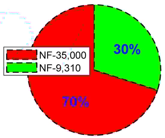
Figure 2.
Normal Form (NF) computation time for full and reduced models.
4.3. Analysis of Case 1
Figure 3a shows the active power response of machine 1 after fault is cleared. Machine 1 is used because it is closest to the fault point. Under this condition, the system is more or less linear. This is revealed by the FFT spectrum in Figure 3b which shows that nonlinear interactions are not strong since the spectrum is dominated by the approximate linear modes. For example, the highest peak corresponds to a frequency of 8.9 rad/s which is approximately mode with frequency 8.94 rad/s in Table 1. This is followed by a peak with frequency 3.9 rad/s which is approximately mode with frequency of 4.03 rad/s in Table 1. The frequency, 17.6 rad/s which also appears in Figure 3b does not exist among the linear modes in Table 1 and must come from modal interaction. Note that, to compute the FFT spectrum, the instant of time for initial conditions should be chosen such that all limiting action by controllers in the system must have ceased after the clearance of the fault.

Figure 3.
(a) Machine 1 active power response for case 1. (b) Fast fourier transform (FFT) spectrum of machine 1 active power for case 1 showing less severe nonlinear effects.
In order to predict which mode is likely responsible for the interaction leading to the unknown frequency in Figure 3b, the indices discussed in Section 2.1.1 and Section 2.1.2 are computed. These indices are listed in Table 2 and Table 3 for 2nd and 3rd order nonlinearities respectively. In Table 2, among the oscillatory modes, mode 4(5) has the largest N2LI and N2II indices. This is followed by modes 17(18) and 13(14). Others have smaller values. This observations suggest that effect of 2nd order nonlinearity on mode 4(5) may be significant. In Table 3 mode 4(5) also has the highest N3LI and N3II among all the oscillatory modes. However, its N3II value is very small compared to the 2nd order value. This observation suggests, perhaps a less significant interaction of 3rd order. From Table 2 and Table 3, one can predict that mode 4(5) is most likely to lead to significant nonlinear interaction. A detailed NF study on mode 4(5) is likely to reveal the mode combination leading to 17.6 rad/s observed in Figure 3b, but since this frequency has negligible amplitude (i.e., 11 dB), the system condition can be assumed linear.
Table 2.
2nd-order NF indices for modal interaction.
Table 3.
3rd-order NF indices for modal interaction.
4.4. Analysis of Case 2
In case 2, the stress is increased and more nonlinearity is induced on the system. The active power response of machine 1 is shown in Figure 4a and its FFT spectrum in Figure 4b. The FFT spectrum shows existence of significant nonlinear interactions whose sources have to be explained. For instance, the frequencies 3.9 rad/s, 8.9 rad/s, and 13.4 rad/s approximately correspond to the linear modes 8(9), 6(7), and 4(5) which have frequencies 4.03 rad/s, 8.94 rad/s, and 13.63 rad/s respectively in Table 1. However, 17.6 rad/s frequency which had negligible amplitude in case 1 now has amplitude of 36 dB and does not correspond to any linear frequency in Table 1. This is also the case of 26.8 rad/s frequency appearing with amplitude of 33 dB higher than the amplitude of the linear frequency 3.9 rad/s. To unravel the sources of these frequencies in Figure 4b, a detailed NF analysis is performed next.
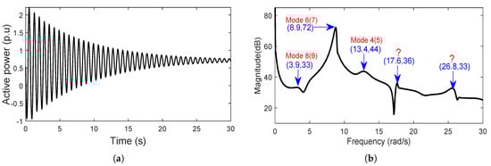
Figure 4.
(a) Machine 1 active power response for case 2. (b) FFT spectrum of machine 1 active power for case 2 showing less severe nonlinear effects.
Qualitative NF Analysis of Case 2
In this section the detailed analyses based on two NF models (i.e., NF-35,000 and NF-9310) are compared. As earlier revealed by Table 2 and Table 3, mode 4(5) is more likely to cause significant modal interactions. It was also established from Table 3 that 3rd order interactions for the studied system may be weak. Hence, only detailed analysis of mode 4(5) is presented, although all other modes were studied. Also only 2nd order modal interaction coefficients () were examined in detail for both NF-35,000 and NF-9310 models.
The nonlinear persistence measures, and together with the interaction coefficients associated with mode 4(5) are listed in Table 4 in descending order of the interaction coefficients. There are numerous interactions involving mode 4(5), so only first few ones are presented.
Table 4.
NF-35,000—Quantitative Measures of combination Modes for Fundamental Mode 4(5).
The largest interaction coefficient corresponds to a combination of eigenvalues 5 and 17 (i.e., − j13.62) which has settling time almost equal to that of the dominant mode (i.e., 3.68 s) and large . However, the new frequency is very near to the linear frequency 13.63 rad/s and is difficult to differentiate by FFT if it appears in the response. Moreover, the modal persistence is close to 1 (i.e., 0.899) hence, it may not even be observed in the response. The combination of eigenvalues 5 and 9 (i.e., − j13.63 − 0.84 − j4.03 = − j17.66) has relatively large interaction coefficient (1.579) and low (0.549) with settling time well above half that of the dominant mode (i.e., 1/2 × 3.68s), and relatively high . These observations indicate that mode 4(5) is interacting nonlinearly with mode 8(9). Notice that the new frequency 17.66 rad/s is approximately observed in the FFT spectrum of Figure 4b (i.e., 17.6 rad/s). Also, down the table, there is a self combination of eigenvalues 5 and 5 (i.e., − j13.63 − 1.02 − j13.63 = − j27.26) which leads to a frequency of 27.26 rad/s, approximate value of the 26.8 rad/s appearing in the spectrum. However, its interaction coefficient is relatively small (0.227) with relatively small value of (0.113). This is consistent with Figure 4b where 26.8 rad/s frequency has low amplitude. If the test system Figure 1 is considered a two-area system, it is seen that mode 4(5) which is associated with area 2 interacts with control mode 8(9) in area 1. Control-wise, in placement of PSS to damp mode 4(5), effect of its interaction with controls in area 1 should be considered in its optimization formulation. Although, the interactions of electromechanical modes with the control modes in the same area should have more adverse effects.
The above analysis is repeated but now with NF-9310 model and the results are listed in Table 5. It is clear from the table that the reduced model identifies correctly the same eigenvalue combinations leading to the observed frequencies in the FFT spectrum. There are some slight deviations in the values of the interaction index () in both cases due to different NF initial conditions.
Table 5.
NF-9310—Quantitative Measures of combination Modes for Fundamental Mode 4(5).
It is important to recall at this point that interactions are detected by comparing the relative magnitudes of the defined indices in each case. Hence, the actual values of these indices do not have to be the same but the information they provide are same for the same case. These indices depend on NF initial condition which in turn depends on the number of h-coefficients considered. Note that the main idea of NF is to at least simplify the system nonlinearity, which implies that the values computed depend on what level the system is simplified to. So, even in full NF, not all h-coefficients computations are possible when resonance occurs. The NF initial conditions are determined only using the possible h-coefficients.
4.5. Relevance of NF Modal Interaction in Power System Control Designs
A common method for siting PSS in power system is the mode-in-state participation factor analysis [43]. Also, in stability studies, attention is more on those modes that participate actively in the stability states (i.e., voltage and angle). In this section, nonlinear participation factor analysis is presented just for the two angle states to emphasize the correction that NF adds to linear analysis. 3rd order NF analysis leads to three types of participation factors: 1-eigenvalue participation factor [6,38,40] which is a correction of the linear one and measures the participation of a single eigenvalue to a state; 2-eigenvalue participation factor [6,38,40] which measures the participation of two eigenvalues combination to a state; and 3-eigenvalue participation factor [40] which measure the participation of three eigenvalues combination to a state. The above references provide details of their evaluations.
Figure 5a,c respectively show the 1-eigenvalue participation factors for relative angles of machines 1 and 2 which were obtained from linear analysis, 2nd NF, and 3rd NF. It can be been seen that the linear analysis under-estimates the contributions of certain eigenvalues. For example, the contributions of eigenvalues 17–20 are not captured at all by the linear analysis, while the contributions of eigenvalue 15 (for machine1) and eigenvalues 13–15 (for machine 2) are far under-estimated. This lack of information may lead to improper control designs or poor placement of PSS. The 2nd and 3rd order 1-eigenvalue corrections are similar as the effect of 3rd order interactions are not very strong in the studied case. Figure 5b,d show respectively the 2-eigenvalue participation factors for machines 1 and 2.

Figure 5.
(a) 1-eigenvalue mode-in-state participation factors to machine 1 relative angle. (b) 2-eigenvalue participation factors to machine 1 relative angle. (c) 1-eigenvalue participation factors to machine 2 relative angle. (d) 2-eigenvalue participation factors to machine 2 relative angle. (e) 3-eigenvalue participation factors to machine 2 relative angle. (f) 3-eigenvalue participation factors to machine 2 relative angle.
Worthy of note is that the eigenvalue combination due to modal interactions can sometimes participate more than the dominant mode. For example, the highest participating mode to machine 2 is mode 4(5), however, in Figure 5d, it is clear that some interactions of this mode have more participation than single mode 4(5). Similar observation has been made in [6]. Figure 5e,f show respectively the 3-eigenvalue participation factors for machines 1 and 2. Here, the 3-eigenvalue participation are not very strong as the bars are far below that of the dominant modes.
Normally PSS is sited in the area with highest participation factor. As seen in the previous section, interaction can exist between modes in two different areas. The area of the newly formed mode is unclear, should it participate more. All these have to be factored in, while designing controls for stressed power systems. A knowledge of interacting modes could be used in nonlinear control of converters in the emerging 100% PE grids.
5. Discussion
In this section, major implications of the results presented in Section 4 are discussed as follows:
- The results illustrate that the proposed method can significantly reduce the computational burden in NF applications. This is depicted with the pie chart shown in Figure 2, where the computation time using the proposed method occupies a sector of 30% against the conventional technique which occupies 70%. In [6], 2nd order modal interaction was studied with a model that has 27 eigenvalues of which 13 are real. In the interpretation of the results, the interactions involving real modes were ignored, which implies a huge computational waste. If this model is to be considered for 3rd order NF study, it will generate 108,864 coefficients. However, with the proposed method, this model will only have 9310 coefficients, a computational saving factor of 12.
- The results show that stressed power system leads to nonlinear interactions of modes. This can be seen for example in case 1 where less severe fault led to spectrum of Figure 3b with no significant interaction, whereas in case 2 where the stress increases, the nonlinearity increases and the modal interaction becomes apparent in the spectrum of Figure 4b. NF analysis is able to identify these interactions as revealed in Table 4 and Table 5. These observations corroborate previous research on modal interaction [6]. A significant new contribution is the use of fewer terms to perform the same analysis. This contribution is especially pertinent in view of fully PE grids. In PE grids there are several modes that decay very fast. The treatment of real modes proposed in this paper may be extended to such very fast modes to further simplify NF application to PE grids.
- The results of the participation factor analyses in Figure 5a–f show the correction to the linear participation factor due to the addition of higher order terms. Reference [14] reported a case where PSS location using nonlinear participation factors outperforms the location using linear participation factor.
- As shown in Figure 5d, the combination modes may participate more than the fundamental modes. Hence, as the disturbance becomes significant, the stability/instability may not be completely determined by single eigenmodes without their interactions. Reference [5] has reported a case where single eigenvalue showed instability but the 3rd order interaction maintained the stability of the system.
- Since the idea proposed in this work addresses specific case of NF application (i.e., modal interaction) its potency for other NF applications such as stability studies is not guaranteed.
- The results indicate that avoiding the interactions associated to the real modes does not compromise the effectiveness of NF modal interaction analysis. This, however, does not mean that all other remaining interactions are nonlinearly significant.
Practical Concerns
It is obvious that the proposed method significantly reduces the computation needed to apply NF to power system, however the following practical concerns are worthy of discussion:
- A major concern is the implication of the proposed method in a large system. Even with the reduction proposed in this paper, the number of nonlinear terms will still be enormous in the case of large system. It is important to state that the approach proposed here is one out of many steps needed to apply NF to large systems. As stated before, the reduction cannot be limited to interactions involving aperiodic (real) modes, but more information is needed to further the reduction to interactions involving oscillatory modes. Although general application of NF to unreduced large system remains difficult, it is good to note that the proposed reduction is based on the physics of the modes and thus, can be applied to system of any size. The authors are working on several ideas, to advance NF to large system. At the moment, reducing the network and focusing on a particular area of the network is the approach to attempt large system (already used in [44] for system with over 300 generators).
- Another valid argument could be if the usefulness of NF analysis is worth the computations involved, given that the time domain analysis could identify the interaction of nonlinear dynamics. It is good to emphasise that NF analysis just like other analytical methods, does not replace time domain analysis but complements it. Time domain analysis can identify the interactions of nonlinear dynamics but the exact natures of these interactions are unclear. Moreover, analytical parameters needed for power system control designs are not as apparent as with analytical methods. It lacks in qualitative information about the system. The nonlinear participation factor analysis helps to know from where comes the interaction. Other analytical information for the power system control designs are not exhaustively available with time domain analysis. NF analysis should be used when some phenomena are difficult to explain with the time domain analysis. Also, indices are needed based on the system condition, to know a priori that it is gainful embarking on NF analysis to avoid computational loss. These indices should be developed. The authors are optimistic that a well developed selective NF application will position it as always very useful tool.
6. Conclusions
In this paper, a method for reducing Normal Form computation by focusing only on some selected terms is proposed. The proposed method consists in neglecting interaction associated to real eigenvalues in the building of NF model. This treatment drastically reduces the computational burden and accelerates the study of modal interaction. The extension of linear analysis to nonlinear participation factors arising from the modal interactions are also presented.
It is important to note that the present work is at investigative stage. In order to make a more global conclusion on the proposed method, further investigations on larger systems and several contingencies are recommended. Future work will investigate these concerns. The main perspective of this work is to extend NF application to the study of large grids, especially the emerging PE grids. This is possible if the computation is sufficiently reduced.
Author Contributions
Conceptualization, N.S.U.; methodology, N.S.U.; validation, X.K., B.M., and O.T.; writing—original draft preparation, N.S.U.; writing—review and editing, N.S.U.; supervision, X.K., B.M., and O.T. All authors have read and agreed to the published version of the manuscript.
Funding
This research was funded by Tertiary Education Trust Fund (TETFund) of Nigeria. The APC was funded by L2EP, Lille France.
Conflicts of Interest
The authors declare no conflict of interest.
Abbreviations
The following abbreviations are used in this manuscript:
| AVR | Automatic voltage regulator |
| DAE | Differential-algebraic equation |
| EV | Electric vehicle |
| FFT | Fast fourier transform |
| HOS | Higher order spectra |
| KMD | Koopman mode decomposition |
| LS | Least square |
| MS | Modal series |
| NF | Normal Form |
| PE | Power electronics |
| PSS | Power system stabilize |
| RE | Renewable energy |
| SEP | Stable equilibrium point |
| SSA | small-signal analysis |
References
- Un-Noor, F.; Padmanaban, S.; Mihet-Popa, L.; Mollah, M.N.; Hossain, E. A comprehensive study of key electric vehicle (EV) components, technologies, challenges, impacts, and future direction of development. Energies 2017, 10, 1217. [Google Scholar] [CrossRef]
- Nguyen, M.; Saha, T.; Eghbal, M. Impact of high level of renewable energy penetration on inter-area oscillation. In Proceedings of the Australasian Universities Power Engineering Conference (AUPEC), Brisbane, QLD, Australia, 25–28 September 2011; pp. 1–6. [Google Scholar]
- You, S.; Kou, G.; Liu, Y.; Zhang, X.; Cui, Y.; Till, M.; Yao, W.; Liu, Y. Impact of High PV Penetration on the Inter-Area Oscillations in the U.S. Eastern Interconnection. IEEE Access 2017, 5, 4361–4369. [Google Scholar] [CrossRef]
- Shair, J.; Xie, X.; Wang, L.; Liu, W.; He, J.; Liu, H. Overview of emerging subsynchronous oscillations in practical wind power systems. Renew. Sustain. Energy Rev. 2019, 99, 159–168. [Google Scholar] [CrossRef]
- Tian, T.; Kestelyn, X.; Thomas, O.; Amano, H.; Messina, A.R. An Accurate Third-Order Normal Form Approximation for Power System Nonlinear Analysis. IEEE Trans. Power Syst. 2018, 33, 2128–2139. [Google Scholar] [CrossRef]
- Sanchez-Gasca, J.J.; Vittal, V.; Gibbard, M.J.; Messina, A.R.; Vowles, D.J.; Liu, S.; Annakkage, U.D. Inclusion of higher order terms for small-signal (modal) analysis: Committee report-task force on assessing the need to include higher order terms for small-signal (modal) analysis. IEEE Trans. Power Syst. 2005, 20, 1886–1904. [Google Scholar] [CrossRef]
- Nayfeh, A.H. The Method of Normal Forms, 2nd ed.; WILEY-VCHVerlag GmbH&Co. KGaA: Weinheim, Germany, 2011. [Google Scholar]
- Jang, G.; Vittal, V.; Kliemann, W. Effect of nonlinear modal interaction on control performance: Use of normal forms technique in control design. II. Case studies. IEEE Trans. Power Syst. 1998, 13, 401–407. [Google Scholar] [CrossRef]
- Lomei, H.; Assili, M.; Sutanto, D.; Muttaqi, K. A New Approach to Reduce the Non-Linear Characteristics of a Stressed Power System by Using the Normal Form Technique in the Control Design of the Excitation System. IEEE Trans. Ind. Appl. 2017, 53, 492–500. [Google Scholar] [CrossRef]
- Wu, F.X.; Wu, H.; Han, Z.X.; Gan, D.Q. Validation of power system non-linear modal analysis methods. Electr. Power Syst. Res. 2007, 77, 1418–1424. [Google Scholar] [CrossRef]
- Starrett, S.K. Nonlinear measures of mode-machine participation. IEEE Trans. Power Syst. 1998, 13, 389–394. [Google Scholar] [CrossRef]
- Amano, H.; Inoue, T. A New PSS Parameter Design Using Nonlinear Stability Analysis. In Proceedings of the IEEE Power Engineering Society General Meeting, Tampa, FL, USA, 24–28 June 2007; pp. 1–8. [Google Scholar]
- Liu, S.; Messina, A.R.; Vittal, V. Assessing placement of controllers and nonlinear behavior using normal form analysis. IEEE Trans. Power Syst. 2005, 20, 1486–1495. [Google Scholar] [CrossRef]
- Liu, S.; Messina, A.R.; Vittal, V. A normal form analysis approach to siting power system stabilizers (PSSs) and assessing power system nonlinear behavior. IEEE Trans. Power Syst. 2006, 21, 1755–1762. [Google Scholar] [CrossRef]
- Amano, H.; Kumano, T.; Inoue, T. Nonlinear stability indexes of power swing oscillation using normal form analysis. IEEE Trans. Power Syst. 2006, 21, 825–834. [Google Scholar] [CrossRef]
- Amano, H.; Kumano, T.; Inoue, T.; Taniguchi, H. Proposal of nonlinear stability indices of power swing oscillation in a multimachine power system. Electr. Eng. Jpn. 2005, 151, 16–24. [Google Scholar] [CrossRef]
- Martinez, I.C.; Messina, A.R.; Barocio, E. Higher-order normal form analysis of stressed power systems: A fundamental study. Electr. Power Compon. Syst. 2004, 32, 1301–1317. [Google Scholar] [CrossRef]
- Martínez, I.; Messina, A.R.; Vittal, V. Normal form analysis of complex system models: A structure-preserving approach. IEEE Trans. Power Syst. 2007, 22, 1908–1915. [Google Scholar] [CrossRef]
- Wang, B.; Sun, K.; Xu, X. Nonlinear Modal Decoupling Based Power System Transient Stability Analysis. IEEE Trans. Power Syst. 2019, 34, 4889–4899. [Google Scholar] [CrossRef]
- Saha, S.; Fouad, A.A.; Kliemann, W.H.; Vittal, V. Stability boundary approximation of a power system using the real normal form of vector fields. IEEE Power Eng. Rev. 1997, 17, 69. [Google Scholar] [CrossRef]
- Kshatriya, N.; Annakkage, U.; Gole, A.; Fernando, I. Improving the Accuracy of Normal Form Analysis. IEEE Trans. Power Syst. 2005, 20, 286–293. [Google Scholar] [CrossRef]
- Modir Shanechi, H.; Pariz, N.; Vaahedi, E. General Nonlinear Modal Representation of Large Scale Power Systems. IEEE Trans. Power Syst. 2003, 18, 1103–1109. [Google Scholar] [CrossRef]
- Abdollahi, A.; Pariz, N.; Shanechi, H.M. Modal series method for nonautonomous nonlinear systems. In Proceedings of the IEEE International Conference on Control Applications, Singapore, 1–3 October 2007; pp. 759–764. [Google Scholar]
- Wang, Z.; Huang, Q. A Closed Normal Form Solution under Near-Resonant Modal Interaction in Power Systems. IEEE Trans. Power Syst. 2017, 32, 4570–4578. [Google Scholar] [CrossRef]
- Netto, M.; Susuki, Y.; Mili, L. Data-Driven Participation Factors for Nonlinear Systems Based on Koopman Mode Decomposition. IEEE Control Syst. Lett. 2019, 3, 198–203. [Google Scholar] [CrossRef]
- Hernandez-Ortega, M.A.; Messina, A.R. Nonlinear Power System Analysis Using Koopman Mode Decomposition and Perturbation Theory. IEEE Trans. Power Syst. 2018, 33, 5124–5134. [Google Scholar] [CrossRef]
- Cossart, Q.; Colas, F.; Kestelyn, X. Model reduction of converters for the analysis of 100% power electronics transmission systems. In Proceedings of the IEEE International Conference on Industrial Technology, Lyon, France, 20–22 February 2018; pp. 1254–1259. [Google Scholar]
- MIGRATE. Horizon 2020 Work Programme 2018–2020. Available online: https://www.h2020-migrate.eu/ (accessed on 17 September 2019).
- Marinescu, B.; Mallem, B.; Rouco, L. Large-scale power system dynamic equivalents based on standard and border synchrony. IEEE Trans. Power Syst. 2010, 25, 1873–1882. [Google Scholar] [CrossRef]
- Marinescu, B.; Mallem, B.; Rouco, L. Model reduction of interconnected power systems via balanced state-space representation. In Proceedings of the 2007 European Control Conference (ECC 2007), Kos, Greece, 2–5 July 2007; pp. 4165–4172. [Google Scholar]
- Belhocine, M.; Marinescu, B. A mix balanced-modal truncations for power systems model reduction. In Proceedings of the 2014 European Control Conference (ECC 2014), Strasbourg, France, 24–27 June 2014; pp. 2721–2726. [Google Scholar]
- Ugwuanyi, N.S.; Kestelyn, X.; Thomas, O.; Marinescu, B. A Novel Method for Accelerating the Analysis of Nonlinear Behaviour of Power Grids using Normal Form Technique. In Proceedings of the Innovative Smart Grid Technologies Europe (ISGT Europe), Bucharest, Romania, 29 September–2 October 2019. [Google Scholar]
- Ugwuanyi, N.S.; Kestelyn, X.; Thomas, O.; Marinescu, B. Selective Nonlinear Coefficients Computation for Modal Analysis of The Emerging Grid. In Proceedings of the Conference des Jeunes Chercheurs en Génie Eléctrique, Ile d’Oléron, France, 11–14 June 2019. [Google Scholar]
- Messina, A.R.; Vittal, V. Assessment of nonlinear interaction between nonlinearly coupled modes using higher order spectra. IEEE Trans. Power Syst. 2005, 20, 375–383. [Google Scholar] [CrossRef]
- Wang, B.I.N.; Sun, K.A.I. Nonlinear Modal Decoupling of Multi-Oscillator Systems With Applications to Power Systems. IEEE Access 2018, 6, 9201–9217. [Google Scholar] [CrossRef]
- Wang, Z.; Huang, Q. Study on an improved Normal Form solution and reduced-order mode reconstruction in power system. In Proceedings of the IEEE Region 10 Annual International Conference, Proceedings/TENCON, Macao, China, 1–4 November 2015. [Google Scholar]
- Ugwuanyi, N.S.; Kestelyn, X.; Thomas, O.; Marinescu, B.; Messina, A.R. A New Fast Track to Nonlinear Modal Analysis of Power System Using Normal Form. IEEE Trans. Power Syst. 2020. [Google Scholar] [CrossRef]
- Jang, G.; Vittal, V.; Kliemann, W. Effect of nonlinear modal interaction on control performance: Use of normal forms technique in control design. I. General theory and procedure. IEEE Trans. Power Syst. 1998, 13, 401–407. [Google Scholar] [CrossRef]
- Dobson, I.; Barocio, E. Scaling of normal form analysis coefficients under coordinate change. IEEE Trans. Power Syst. 2004, 19, 1438–1444. [Google Scholar] [CrossRef]
- Huang, Q.; Wang, Z.; Zhang, C. Evaluation of the effect of modal interaction higher than 2nd order in small-signal analysis. In Proceedings of the 2009 IEEE Power and Energy Society General Meeting, PES ’09, Calgary, AB, Canada, 26–30 July 2009; pp. 1–6. [Google Scholar]
- Sauer, P.W.; Pai, M.A. Power System Dynamics and Stability; Prentice Hall: Upper Saddle River, NJ, USA, 1998; p. 357. [Google Scholar]
- Milano, F. An open source power system analysis toolbox. IEEE Trans. Power Syst. 2005, 20, 1199–1206. [Google Scholar] [CrossRef]
- Hashlamoun, W.A.; Hassouneh, M.A.; Abed, E.H. New results on modal participation factors: Revealing a previously unknown dichotomy. IEEE Trans. Autom. Control 2009, 54, 1439–1449. [Google Scholar] [CrossRef]
- Vittal, V.; Kliemann, W.; Chapman, D.G.; Silk, A.D.; Xni, Y.; Sobajic, D.J. Determination of generator groupings for an islanding scheme in the manitoba hydro system using the method of normal forms. IEEE Trans. Power Syst. 1998, 13, 1345–1351. [Google Scholar] [CrossRef]
© 2020 by the authors. Licensee MDPI, Basel, Switzerland. This article is an open access article distributed under the terms and conditions of the Creative Commons Attribution (CC BY) license (http://creativecommons.org/licenses/by/4.0/).