Abstract
This study discusses the evaluation of oscillatory stability based on the synchronizing and damping torque coefficients for a single-machine system connected to an infinite bus (SMIB). Particle swarm optimization (PSO) technique is used to determine and values and subsequently identify the oscillatory stability conditions in the SMIB. The ability of PSO is compared with those of evolutionary programming (EP) techniques and artificial immune system (AIS). The least square (LS) method is selected as the benchmark for and values determined by PSO, EP, and AIS. Simulation results show that PSO successfully estimated and values closest to LS compared with EP and AIS. PSO also uses lower computational time compared with those of the two other techniques. The proposed technique is suitable for solving oscillatory stability problems based on the determination of eigenvalues and minimum damping ratio.
1. Introduction
The increase in population worldwide has major implications to electricity consumption. Power generation companies always innovate to ensure that the energy supply is sufficient and stable. Accordingly, small signal stability is a frequently discussed topic, as reported in [1,2,3,4,5]. This system must be tracked online because its power system operating condition changes over time. Various indicators, such as damping ratio [6,7,8] and damping factor [9], have been proposed to determine the angular stability of a system. However, the eigenvalues obtained from the entire mathematical model of the system are needed to calculate these two indicators. In this study, the synchronizing and damping torque coefficients were introduced to verify system stability. and can be calculated on the basis of the information from three rotor responses, namely the changes in rotor angle, ; rotor speed, ; and electromechanical torque, . A system is considered stable when the values of and are positive [10,11,12]. However, the system is considered unstable when one of the values is negative.
Least square (LS) method is often used to calculate and values of a system by using a static parameter estimation approach [13,14,15]. However, the LS method needs a large data set to obtain the correct values. Extensive data collection also requires long computation time. Monitoring the oscillation period is also critical because the occurrence of slight data error leads to inaccurate and values. Thus, heuristic techniques are introduced to solve this problem. and values will be optimized from the beginning of the data until constant and values are obtained. Therefore, only a portion of the data is necessary for estimating and . Minor data errors do not significantly affect the determination of and values.
In recent years, the use of artificial intelligence (AI) technology has become the preferred option in solving power system problems. The use of AI is introduced to solve the optimum values of a system or condition particularly in the fields of economic dispatch, capacitor placement and sizing, and assessment and improvement of voltage and oscillatory stability. Artificial neural networks [16,17], evolutionary programming (EP) [18,19,20], artificial immune systems (AIS) [21,22,23], and ant colony optimization (ACO) [24,25,26] are AI approaches that are commonly used in power systems. The EP algorithm is modeled on the biological evolution process of solving a complex problem. The main features of EP include the mutation process of the next generation and the selection of increasingly powerful genes. The AIS algorithm uses a concept similar to that of EP. Although both concepts are biologically based on living things, EP focuses on the evolution of living things, whereas AIS adopts the concept of the living immune system. The difference between AIS and EP algorithms is that AIS has an additional process of cloning called the clonal selection algorithm. However, the ACO approach is inspired by the true behavior of ants while searching for food and interacting with fellow ants. In ACO, artificial ants (the search agent) will communicate by using pheromones, which guide the searcher ants to solve the calculation problem by tracking the best route. Meanwhile, the particle swarm optimization (PSO) [27,28,29,30] concept mimics the movements of a herd, such as the behavior of schooling fish and swarming insects. This technique was originally founded based on the population of random particles, in which every particle is a potential solution. PSO can make adjustments to obtain balance between global and local explorations during the search process. This feature makes the PSO suitable for overcoming the problems caused by initial convergence and improving the ability to search.
This study presents the techniques for determining oscillatory stability based on the estimation of twin indicators called synchronizing and damping torque coefficients. A single machine linked to a large bus network or infinite bus (SMIB) is selected as the test system. The changes in rotor angle, ; rotor speed, ; and electromechanical torque, are used to determine and values. This optimization process aims to minimize the error of both torque coefficients. In this study, the PSO technique was selected as the heuristic technique for solving this optimization problem. The results in PSO will be compared with those of EP and AIS. From the simulation using MATLAB, these three heuristic techniques will be compared based on the accuracy of the torque coefficient, the amount of iteration for the simulation process, and simulation time. The eigenvalues and minimum damping ratio , are also used to verify the system stability.
2. Materials and Methods
2.1. Oscillatory Stability Assessment
In oscillatory instability detection studies, early detection can provide the system time to improve its stability and prevent further system instability and eventual collapse. This study introduces and as the indicators for determining system stability. and are estimated periodically whenever new data are received from the system. To validate the result, and are estimated using the LS calculation method. Eigenvalue and damping ratio analysis were also conducted to verify the accuracy of the results.
2.1.1. and
In the oscillatory stability analysis, electromechanical torque can be expressed in the form of synchronous and damping torque components. The relationship among the rates of change in the estimated electromechanical torque, ; rotor angle, ; in rotor speed, ; synchronizing torque coefficients, ; and damping torque coefficients, can be expressed as follows:
The stability evaluation of a linear system can be predicted based on and values. A stable system is guaranteed when and values are positive. Figure 1 illustrates a stable angle stability as resulted from the positive values of and .
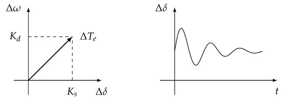
Figure 1.
Complex plane of and response in stable condition.
If the linear system has a positive and a negative value, then the system is under an unstable oscillatory condition, which is due to lack of adequate damping torque. The effect of the oscillatory instability condition can be detected from the increment of amplitude oscillations of the rotor. Figure 2 shows the unstable conditions of angle stability from the positive value and the negative value.
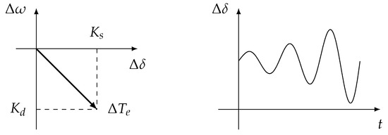
Figure 2.
Complex plane of and response for unstable oscillatory condition.
Non-oscillatory instability occurs when and show negative and positive values, respectively, because the absence of automatic voltage regulators results in the lack of sufficient synchronizing torque. This condition can be verified based on the steady increment of rotor angle response. Figure 3 presents the unstable conditions for angle stability from the negative and positive value.
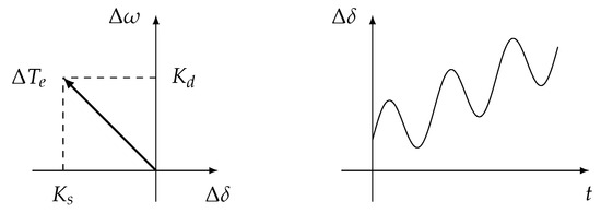
Figure 3.
Complex plane of and response for unstable non-oscillatory condition.
2.1.2. LS Method
Several methods have been proposed to estimate the value of and which involved optimization approach. LS method can be one of the possible techniques in addressing this phenomenon, which has been used as static parameter estimation as reported in [18]. The LS method is a form of mathematical analysis that calculates the most appropriate solution based on a data set. In this study, the LS technique is used to minimize the sum of the squares of errors . Error is the difference between the changes in the estimated electromechanical torque and the changes in the electromechanical torque . From the previous equation, can be calculated based on the values of and from the data set, and also estimated values of and . The equation of is as follows:
For the overdetermined matrix system , the sum of the squared value of can be defined as the following function :
where N is the number of experimental samples.
To minimize , and need to be calculated throughout the entire oscillation period. The solution for this equation can be given as
Matrix is invertible. Thus, the solution of x is given by
The torque coefficients and can be calculated by solving Equation (7). Although the calculated values are accurate, the application of the LS method requires data for the entire swing [5,6]. The need for such large data collection also requires a long calculation time. Accordingly, a new indicator is needed.
2.1.3. Eigenvalue and Damping Ratio
There are various methods for determining the stability of a system, including the calculation of eigenvalues and damping ratios. Eigenvalues are derived from matrix arrays by linear system equations. However, the damping ratio is derived using a combination of real and imaginary values of eigenvalues. Eigenvalues and damping ratios are often used as indicators for measuring the stability of a system, as described in [18]. Eigenvalues of a matrix representing a linear system are obtained as follows:
where is a matrix, is a vector, and is the eigenvalues matrix . To determine the eigenvalues, Equation (8) can be written as
The eigenvalues of are the n solutions of . The ith eigenvalue of a matrix representing a linear system are obtained as follows:
where and are the real and imaginary parts of the ith eigenvalue, respectively. The negative real part of all eigenvalues indicates that a linear system is stable. The damping ratio, , for the ith eigenvalue is defined as [31,32]:
The linear system is certainly stable when all the damping ratios have positive values. For simplification, only the minimum damping ratio, , for the linear system is selected to verify the result.
2.2. Test System
In this study, an SMIB system is selected for evaluation. , , and are generated in a MATLAB Simulink environment based on the block diagram of the SMIB model. According to Equation (1), the estimated electric torque, , is calculated by using the generated sample data for and .
2.2.1. Philips–Heffron Model
Figure 4 shows the SMIB system with a classical generator model.
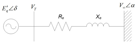
Figure 4.
SMIB system.
Here, and are resistance and reactance of the transmission line, respectively. and are terminal bus and infinite bus voltages, respectively. and are the rotor angles at terminal bus and infinite bus, respectively. is the generator terminal voltage. The equations for rotor acceleration, rotor angle, and the field circuit are presented as follows [33,34]:
Here, is the change of rotor acceleration, is the change of rotor angle, is the change of the field circuit, is a field voltage, is the rotor mechanical torque, H is the machine inertia constant, and D is the machine damping coefficients.
According to Equations (12)–(14), the Philips–Heffron block diagram model of SMIB is developed and shown in Figure 5 [1]. This figure illustrates that the constant K represents several variables, such as the electric torque, rotor speed, and rotor angle. From the Philips–Heffron block diagram model, the following are developed:
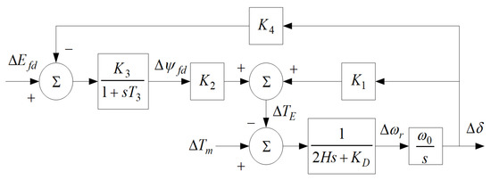
Figure 5.
Philips–Heffron block diagram model.
Here, and are resistance and reactance of field circuit, respectively. and are the generator d-axis and q-axis saturated value of mutual inductance, respectively. is total q-axis reactance of the system. is total system resistance. is the initial rotor angle. is the field circuit reactance.
The function of the system parameters is separated into two system matrices, namely A and B. The details in the calculation of matrices A and B are presented in [18].
2.2.2. Objective Function
In this study, three optimization techniques, namely EP, AIS, and PSO, are used to determine the values of torque coefficients and . The difference between and is defined as an error. This error is minimized at each iteration by using heuristic techniques when the new and values are calculated. In this study, the objective function is formulated based on the error as follows:
By the implementation of this objective function will ensures that the difference between and versus is close to or equal to 0. This objective function is developed such that the value of J will be in the range 0 and 1, and value 1 is the optimal value. The designed problem in this study can be represented by
These two torque coefficients are simultaneously optimized via the three optimization techniques for the different cases by using the proposed objective function.
2.2.3. Algorithm for and Estimation
The flowchart for and estimation process is shown in Figure 6.
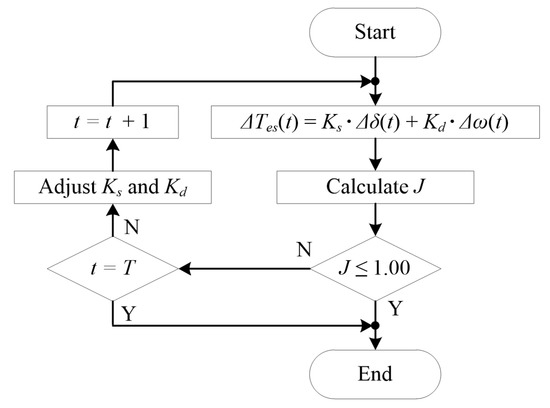
Figure 6.
Flowchart for the estimation process of and .
3. Computational Intelligence Methods for Oscillatory Stability Assessment
In recent years, AI technology has been widely used in solving optimization problems in power systems. Evolutionary computation (EC) is a widely used AI technique. EC models evolutionary processes to develop strategies that seek optimal or almost optimal solutions for specific problems. Examples of EC techniques include EP, genetic algorithm, AIS, and PSO. In this study, AIS, EP, and PSO are selected as optimization techniques.
3.1. PSO
The PSO technique is inspired by the feeding process of certain animals, such as swarming birds and schooling fish. The PSO algorithm begins with initialization, followed by the update of velocity and position, fitness calculation, the best position update, and convergence test. The pseudocode that represents the PSO algorithm is illustrated in Algorithm 1. Detailed explanations of the PSO algorithm process can be found in [28].
In Algorithm 1, k is the number of iterations, i is the number of particles, is the inertia weight, and are the velocity and position for the ith particle, respectively. and are the acceleration coefficients, J is the objective function, as shown in Equation (22), is the personal best position for the ith particle, and is the global best position.
| Algorithm 1 Pseudocode for the PSO algorithm [28]. |
|
3.2. EP
The concept of EP is based on the theory of evolution of life through natural selection. EP is motivated by the process at the evolution stage (parents, mutation, offspring) but without the genetic evolution. The EP algorithm begins with the initialization, followed by the determination of fitness, mutations, combinations of parent and offspring, and ends with selection. Algorithm 2 demonstrates the pseudocode for the EP algorithm [18].
| Algorithm 2 Pseudocode for the EP algorithm [18]. |
|
In Algorithm 2, l is the number of generations, j is the number of populations, is a mutation factor in EP, and and are the parents and offspring for the population, respectively.
3.3. AIS
AIS is an optimization technique that attempts to biologically imitate the human immune system. This concept, which is practiced in the AIS technique, is similar to that of the EP technique. However, AIS has an additional criterion called cloning. The entire process is given in the form of a pseudocode in Algorithm 3 [23].
In Algorithm 3, m is the number of cycles, h is the number of cells, is a mutation factor in AIS, is the precloning of hth cells, is the post-cloning cells, and is the mutated hth cells.
Table 1 lists the parameters used in the PSO, EP, and AIS techniques. The value of these parameters are selected based on the values used in the reference [8].

Table 1.
List of parameters used in PSO, EP and AIS.
| Algorithm 3 Pseudocode for the AIS algorithm [23]. |
|
4. Results and Discussion
This study estimates oscillatory stability by using and in various loading conditions of the SMIB system. The samples of , , and are required in the calculated estimations generated in the MATLAB Simulink environment. EP, AIS, and PSO are used to estimate the values of and . The results are compared with the benchmark values calculated via the LS method. The values of and are also used to justify stability determination. For estimation with AI algorithms and LS, data size used is set to 20 s, while number of samples is set to 400 samples. The value of this 400 samples data proved to be effective for the AI algorithms and LS to make accurate calculations, based on the reference [18]. In this study, the simulation tests are conducted using Intel (R) Core (TM) i7-4770 CPU @ 3.40Ghz processor.
To determine the appropriate population size during the optimization process, the effect of population size for angle stability assessment of SMIB system has been studied. Three different population sizes, namely 5, 20 and 50 population sizes have been tested, using loading condition of P = 0.6 p.u. and Q = 0.7 p.u. The data of synchronizing torque coefficient, , damping torque coefficient, and three different population sizes are tabulated in Table 2.
Table 2.
Results of , and computation time for three different population sizes with P = 0.6 p.u. and Q = 0.7 p.u.
From Table 2, it is clearly shown that the results obtained using PSO and LS are the same when optimized with 20 and 50 populations. The result for optimized using EP at population size of 50 is the same as that computed using LS. This indicates that 50 is the most suitable population size if closeness to LS technique is desired. This result is significant with the result of . It is shown that PSO outperformed AIS and EP since it manages to achieve final solution close to the value obtained by LS. From the computation time point of view, it shows that computation time of optimization process of EP and PSO is proportional to the population size of the simulation. On the other hand, AIS method gives the shortest computation time when the population size is set to 20. This revealed that AIS managed to achieve optimal solution within population size of 20. It was also discovered that the value of fitness is always consistent even the size population is increased up to 50. According to this result, 20 was selected as population size during the optimization process.
In this study, two large events with different cases, namely Events A and B, are evaluated. In Event A, the value of active power, P, is randomly set to 0.5 p.u., whereas reactive power, Q, increases linearly by 0.1 p.u. from 0.1 p.u. to 1.0 p.u. In Event B, Q is set to 0.15 p.u., whereas P decreases by 0.1 p.u. from 1.0 p.u. to 0.1 p.u. The loading condition values are selected because they obtain significant results.
Table 3 presents the values of and estimated by using EP, AIS, PSO, LS, , and for Event A. All the cases show the negative and positive values of and , indicating that all the cases are stable. In each case, a total of 10 replications for the simulation process were performed. The results obtained are consistent and within the range of not more than 1%. The LS method is selected as the standard value for EP, AIS, and PSO estimation methods.
Table 3.
and via EP, AIS, PSO, LS, eigenvalues and for Event A.
The results in Table 3 show that the estimated values of and using the PSO method obtains more accurate values than EP and AIS. Particularly for the data of for Cases A-1, A-4, and A-7, the PSO estimation technique obtains exactly the same values as those calculated via the LS method. The AIS technique achieves the worst results, such that most of the estimated values are different from those calculated with the LS method.
Fitness of the EP, AIS, and PSO methods for Event A is illustrated in graph form in Figure 7. Figure 7a shows that the PSO technique obtains the highest fitness values for all cases. Fitness for EP and AIS are in the range of 0.92 to 0.98, whereas that of PSO is in the range of 0.99 to 1.00. This finding implies that PSO calculates better fitness results than EP and AIS.
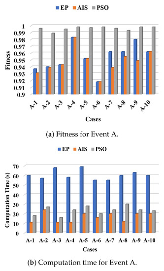
Figure 7.
Fitness and computation time for Event A.
The results of the computation time for Event A for all three estimation techniques are demonstrated in Figure 7b. The graph indicates that EP takes the longest computation time with an average time of approximately 60 s. The AIS method is the fastest among the three techniques because most of the simulation cases achieved an optimal solution below 30 s.
For Event A, PSO achieves better results in the objective function compared with EP and AIS. However, AIS simulates the estimation process in a short computation time and small iteration number. Overall, PSO is the best method in most of the discussed situations. Table 4 tabulates the values of and estimated via EP, AIS, PSO, LS, , and for Event B. From the 10 cases, the first 7 cases show positive and negative , indicating that the first 7 cases are in a stable condition. The three final cases are considered unstable because of the negative value of the minimum damping ratio, , and positive eigenvalues, . The estimated values of and via the LS method supports the result of and . From the estimation process for the first seven cases, which used the LS method, the values of and are positive. These findings indicate that Cases B-1 to B-7 are stable. For Cases B-8, B-9, and B-10, the LS results give negative values for and positive values for , thereby proving that all three final cases are considered non-oscillatory instability cases. In each case, a total of 10 replications for the simulation process were performed. The results obtained are within the range of not more than 1%.
Table 4.
and via EP, AIS, PSO, LS, eigenvalues and for Event B.
From Table 4, PSO method exhibits more comparable results with respect to AIS and EP, particularly for the two final cases, namely Cases B-9 and B-10. In these two cases, the estimated value of using EP and AIS are far deviated from PSO and LS method.
The profile for the fitness of EP, AIS, and PSO method for Event B is presented in Figure 8a. From the graph, the PSO technique acquires the highest fitness values as compared with EP and AIS. The fitness values for EP and AIS are in the range of 0.92 to 0.98, whereas PSO is in the range of 0.99 to 1.00. This finding implies that PSO outperformed EP and AIS in determining the values of and with high accuracy.
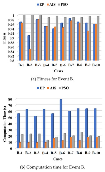
Figure 8.
Fitness and computation time for Event B.
Figure 8b lists the results of computation time for Event B for the EP, PSO, and AIS estimation techniques. EP is the slowest among the three techniques with the computation time in a range of 40–80 s. For the AIS method, 5 out of 10 cases finished the computation process in 20 s.
The results of Event B indicate that PSO can optimize the best value of torque coefficients and . PSO reaches higher fitness values than EP and AIS. AIS obtains better computation time, but EP is computationally burdensome.
5. Conclusions
In this study, an efficient real-time estimation technique of torque coefficients and for solving angle stability problems is proposed. and are estimated on the basis of , , and . The values of and based on the LS technique are selected as the benchmark for evaluating the performance of the proposed optimization method. Overall, PSO is excellent for calculating the values of and because it obtains almost the same values as those calculated via the LS method. Although EP and AIS can determine the stability condition of all the cases, the value differences of and when compared with LS for EO and AIS are larger than those obtained by using PSO. From the perspective of computation time and iterations, AIS obtains the fastest simulation time in this event, followed by PSO and EP. Despite the large iteration number, the time consumed for the PSO simulation process is still minimal and acceptable. From the point of view of population size, the performance of calculation accuracy for all the three techniques significantly increased when simulations are conducted in 20 and 50 population sizes compared with that in 5 population sizes. The computation time consumed and number of iterations increase significantly regardless of the calculation accuracy performance in each optimization technique as the population sizes increase. The results of the last three events suggest that 20 is the recommended population size for calculating the accurate value of and via the PSO technique.
Author Contributions
Conceptualization, N.A.M.K. and I.M.; methodology, N.A.M.K.; software, N.A.M.K.; validation, N.A.M.K. and I.M.; formal analysis, N.A.M.K.; investigation, N.A.M.K.; resources, I.M.; data curation, N.A.M.K.; writing–original draft preparation, A.N.D. and M.H.M.Z.; writing–review and editing, N.A.M.K. and M.H.M.Z.; visualization, N.A.M.K.; supervision, I.M.; project administration, N.A.M.K.; funding acquisition, N.A.M.K. All authors have read and agreed to the published version of the manuscript.
Funding
This work was supported by Ministry of Education Malaysia under code FRGS/1/2018/TK04/UKM/02/7.
Conflicts of Interest
The authors declare no conflict of interest.
Abbreviations
The following abbreviations are used in this manuscript:
| AIS | Artificial Immune System |
| EC | Evolutionary Computation |
| EP | Evolutionary Programming |
| LS | Least Square |
| PSO | Particle Swarm Optimization |
| SMIB | Single-Machine Infinite Bus |
References
- Oh, S.C.; Lee, H.I.; Lee, Y.H.; Lee, B.J. A novel SIME configuration scheme correlating generator tripping for transient stability assessment. J. Electr. Eng. Technol. 2018, 13, 1798–1806. [Google Scholar]
- Wadduwage, D.P.; Annakkage, U.D.; Wu, C.Q. Hybrid algorithm for rotor angle security assessment in power systems. J. Eng. 2015, 2015, 241–251. [Google Scholar] [CrossRef]
- Ali, M.A.S.; Mehmood, K.K.; Kim, C.H. Power system stability improvement through the coordination of TCPS-based damping controller and power system stabilizer. Adv. Electr. Comput. Eng. 2017, 17, 27–36. [Google Scholar] [CrossRef]
- Abbasi, S.M.; Karbalaei, F.; Badri, A. The effect of suitable network modeling in voltage stability assessment. IEEE Trans. Power Syst. 2019, 34, 1650–1652. [Google Scholar] [CrossRef]
- Wei, S.; Yang, M.; Qi, J.; Wang, J.; Ma, S.; Han, X. Model-free MLE estimation for online rotor angle stability assessment with PMU data. IEEE Trans. Power Syst. 2018, 33, 2463–2476. [Google Scholar] [CrossRef]
- Chitara, D.; Niazi, K.R.; Swarnkar, A.; Gupta, N. Cuckoo search optimization algorithm for designing of a multimachine power system stabilizer. IEEE Trans. Ind. Appl. 2018, 54, 3056–3065. [Google Scholar] [CrossRef]
- Islam, N.N.; Hannan, M.A.; Mohamed, A.; Shareef, H. Improved power system stability using backtracking search algorithm for coordination design of PSS and TCSC damping controller. PLoS ONE 2016, 11, e0146277. [Google Scholar]
- Kamari, N.A.M.; Musirin, I.; Hamid, Z.A.; Zaman, M.H.M. Oscillatory stability prediction using pso based synchronizing and damping torque coefficients. Bull. Electr. Eng. Inform. 2018, 7, 331–344. [Google Scholar]
- Yang, B.; Sun, Y. A novel approach to calculate damping factor based delay margin for wide area damping control. IEEE Trans. Power Syst. 2014, 29, 3116–3117. [Google Scholar] [CrossRef]
- Gurrala, G.; Sen, I. Synchronizing and damping torques analysis of nonlinear voltage regulators. IEEE Trans. Power Syst. 2011, 26, 1175–1185. [Google Scholar] [CrossRef]
- Kamari, N.A.M.; Musirin, I.; Othman, M.M. Application of evolutionary programming in the assessment of dynamic stability. In Proceedings of the IEEE 4th International Power Engineering and Optimization Conference, Kuala Lumpur, Malaysia, 23–24 June 2010; pp. 43–48. [Google Scholar]
- Hammoudeh, A.; Al Saaideh, M.I.; Feilat, E.A.; Mubarak, H. Estimation of synchronizing and damping torque coefficients using deep learning. In Proceedings of the IEEE Jordan International Joint Conference on Electrical Engineering and Information Technology, Amman, Jourdan, 9–11 April 2019; pp. 488–493. [Google Scholar]
- De Almeida, M.C.; Garcia, A.V.; Asada, E.N. Regularized least squares power system state estimation. IEEE Trans. Power Syst. 2012, 27, 290–297. [Google Scholar] [CrossRef]
- Xia, Y.; Blazic, Z.; Mandic, D.P. Complex-valued least squares frequency estimation for unbalanced power systems. IEEE Trans. Instrum. Meas. 2015, 64, 638–648. [Google Scholar] [CrossRef]
- Yu, L.; Wang, H.; Che, J.; Lu, J.; Zheng, X. Outliers screening for photovoltaic electric power based on the least square method. In Proceedings of the Chinese Control and Decision Conference, Yinchuan, China, 28–30 May 2016; pp. 2799–2804. [Google Scholar]
- Ymeri, A.; Mujovic, S. Impact of photovoltaic system pPlacement, sizing on power quality in distribution network. Adv. Electr. Comput. Eng. 2018, 18, 107–112. [Google Scholar] [CrossRef]
- Hagmar, H.; Tuan, L.A.; Carlsot, O.; Eriksson, R. On-Line voltage instability prediction using an artificial neural network. In Proceedings of the IEEE Milan PowerTech, Milan, Italy, 23–27 June 2019. [Google Scholar]
- Kamari, N.A.M.; Musirin, I.; Othman, M.M. EP based optimization for estimating synchronizing and damping torque coefficients. Aust. J. Basic Appl. Sci. 2010, 4, 3741–3754. [Google Scholar]
- Kadir, A.F.A.; Mohamed, A.; Shareef, H.; Wanik, M.Z.C. Optimal placement and sizing of distributed generations in distribution systems for minimizing losses and THDv using evolutionary programming. Turk. J. Electr. Eng. Comput. Sci. 2013, 21, 2269–2282. [Google Scholar] [CrossRef]
- Wang, L.; Zhang, Q.; Zhou, A.; Gong, M.; Jiao, L. Constrained subproblems in a decomposition-based multiobjective evolutionary algorithm. IEEE Trans. Evol. Comput. 2016, 20, 475–480. [Google Scholar] [CrossRef]
- Lakshmi, K.; Vasantharathna, S. Hybrid artificial immune system approach for profit based unit commitment problem. J. Electr. Eng. Technol. 2013, 8, 959–968. [Google Scholar] [CrossRef]
- Alonso, F.R.; Oliveira, D.Q.; Zambroni de Souza, A.C. Artificial iImmune systems optimization approach for multiobjective distribution system reconfiguration. IEEE Trans. Power Syst. 2015, 30, 840–847. [Google Scholar] [CrossRef]
- Dudek, G. Artificial immune system with local feature selection for short-term load forecasting. IEEE Trans. Evol. Comput. 2017, 21, 116–130. [Google Scholar] [CrossRef]
- Hamid, Z.A.; Musirin, I.; Rahim, M.N.A.; Kamari, N.A.M. Application of electricity tracing theory and hybrid ant colony algorithm for ranking bus priority in power system. Int. J. Electr. Power Energy Syst. 2012, 43, 1427–1434. [Google Scholar] [CrossRef]
- Rahmat, N.A.; Aziz, N.F.A.; Mansor, M.H.; Musirin, I. Optimizing economic load dispatch with renewable energy sources via differential evolution immunized ant colony optimization technique. Int. J. Adv. Sci. Eng. Inf. Technol. 2017, 7, 2012–2017. [Google Scholar] [CrossRef]
- Suhane, P.; Rangnekar, S.; Mittal, A.; Khare, A. Sizing and performance analysis of standalone wind-photovoltaic based hybrid energy system using ant colony optimization. IET Renew. Power Gener. 2016, 10, 964–972. [Google Scholar] [CrossRef]
- Pijarski, P.; Kacejko, P. Methods of simulated annealing and particle swarm applied to the optimization of reactive power flow in electric power systems. Adv. Electr. Comput. Eng. 2018, 18, 43–48. [Google Scholar] [CrossRef]
- Kamari, N.A.M.; Musirin, I.; Othman, M.M. IPSO based SVC-PID for angle stability enhancement. Int. J. Simul. Syst. Sci. Technol. 2017, 17, 20.1–21.7. [Google Scholar]
- Yang, J.S.; Chen, Y.W.; Hsu, Y.Y. Small-signal stability analysis and particle swarm optimization self-tuning frequency control for an islanding system with DFIG wind farm. IET Gener. Transm. Distrib. 2019, 13, 563–574. [Google Scholar] [CrossRef]
- Hamdan, A.H.; Hashim, F.H.; Mohamed, A.Z.; Zaki, W.M.D.W.; Hussain, A. Modified particle swarm optimization with novel modulated inertia for velocity update. Int. J. Eng. Technol. 2016, 8, 1855–1860. [Google Scholar] [CrossRef][Green Version]
- Mithulananthan, N.; Shah, R.; Lee, K.Y. Small-disturbance angle stability control with high penetration of renewable generations. IEEE Trans. Power Syst. 2014, 29, 1463–1472. [Google Scholar] [CrossRef]
- Kamari, N.A.M.; Musirin, I.; Othman, Z.; Halim, S.A. PSS based angle stability improvement using whale optimization approach. Indones. J. Electr. Eng. Comput. Sci. 2017, 8, 382–390. [Google Scholar] [CrossRef]
- Alkhalaf, S. Modeling the automatic voltage regulator (AVR) using artificial neural network. In Proceedings of the International Conference on Innovative Trends in Computer Engineering, Aswan, Egypt, 2–4 February 2019; pp. 570–575. [Google Scholar]
- Kumar, S.; Kumar, A.; Shankar, G. Crow search algorithm based pptimal dynamic performance control of SVC assisted SMIB system. In Proceedings of the 20th National Power Systems Conference, Tiruchirappalli, India, 14–16 December 2018. [Google Scholar]


© 2020 by the authors. Licensee MDPI, Basel, Switzerland. This article is an open access article distributed under the terms and conditions of the Creative Commons Attribution (CC BY) license (http://creativecommons.org/licenses/by/4.0/).