Article

Thickness Distribution Prediction for Tectonically Deformed Coal with a Deep Belief Network: A Case Study

1
Department of Data Science, School of Computer Science and Technology, China University of Mining and Technology, Xuzhou 221116, China
2
Mine Digitization Engineering Research Center of the Ministry of Education, China University of Mining and Technology, Xuzhou 221116, China
3
Department of Geophysics, School of Resources and Geosciences, China University of Mining and Technology, Xuzhou 221116, China
*
Author to whom correspondence should be addressed.
Energies 2020, 13(5), 1169; https://doi.org/10.3390/en13051169
Submission received: 25 January 2020 / Revised: 18 February 2020 / Accepted: 2 March 2020 / Published: 4 March 2020
(This article belongs to the Section H: Geo-Energy)

Abstract

:
Thickness of tectonically deformed coal (TDC) has positive correlations with the susceptible gas outbursts in coal mines. To predict the TDC thickness of the coalbed, we proposed a prediction method using seismic attributes based on the deep belief network (DBN) and dimensionality reduction. Firstly, we built a DBN prediction model using the extracted attributes from a synthetic seismic section. Next, we transformed the possibly correlated seismic attributes into principal components through principal components analysis. Then, we compared the true TDC thickness with the predicted TDC thicknesses to evaluate the prediction accuracy of different models, i.e., a DBN model, a support vector machine model, and an extreme learning machine model. Finally, we used the DBN model to predict the TDC thickness of coalbed No. 8 in an operational coal mine based on synthetic experiments. Our studies showed that the predicted distribution of TDC thickness followed the regional characteristics of TDC development well and was positively correlated with the burial depth, coalbed thickness, and tectonic development. In summary, the proposed DBN model provided a reliable method for predicting TDC thickness and reducing gas outbursts in coal mine operations.

Graphical Abstract

1. Introduction

Tectonically deformed coal (TDC) is a kind of coal that has experienced physical and chemical damages or deformations due to tectonic movements [1,2]. Conventionally, TDC is far weaker than undeformed coal in strength and elasticity. As is known, TDC development is directly associated with the susceptible gas outbursts in coal mines. The thicker the TDC is, the higher is the probability of gas outbursts. Therefore, coal mining safety is directly related to the occurrence of thick TDC [3,4,5,6,7]. If the TDC thickness of coal beds could be predicted quantitatively and accurately before coal excavation and mining, safe coal mining would be an achievable target for coalmine operators.
Seismic attributes are useful input for reservoir prediction. Among them, the curvature is related to structural development, the amplitude is related to impedance contrast and bed thickness, frequency and bandwidth are related to bed thickness and burial depth, and sweetness and spectral decomposition are related to bed lithology [8,9,10,11]. In the literature, most studies have been focusing on the forecasting of TDC distribution with seismic attribute input [12,13,14]. While the predicted distributions are essential references for coal mining, they provide only indirect parameters for mine planning and mine-disaster prevention. In contrast, TDC thickness could be used directly to predict the gas outbursts in coal mines as it is directly related to structural development, coalbed thickness, and burial depth [1,2,15]. Therefore, it is worthy of exploring the quantitative prediction method for TDC thickness in coal mines.
Machine learning technologies, including a fuzzy neural network (FNN), support vector machines (SVM), and extreme learning machine (ELM), have been used to predict TDC thickness and have achieved valuable results [11,16,17]. However, they have not found wide applications in the coal mining industry due to the limitations in learning speed and modeling capacity.
Recently, deep learning technologies have been widely and successfully used in many areas. Among these technologies, a deep belief network (DBN), proposed by Hinton et al. [18], is a typical deep learning model. During the past two decades, researchers are more interested in DBN because of the invention of efficient layer-by-layer learning technology. In general, the DBN, composed of multiple layers of stochastic and latent variables, is regarded as a special form of Bayesian probabilistic generative model [19]. In comparison with traditional neural networks, DBN has many advantages, including the ability to solve the overfitting problem in training data and obtain a local minimum with less computing. The typical applications of DBN include natural language understanding, classification, and dimensionality reduction [19,20,21].
In this paper, we explored a DBN model with seismic attributes and dimensionality reduction to predict the TDC thickness, based on a synthetic example and testing data from an operational coal mine.

2. Methods

2.1. Dimensionality Reduction

In practical applications, the number of seismic attributes is huge, and the information on seismic attributes is redundant [11]. Consequently, it is compulsory to reduce the dimensionality of seismic attributes before training and prediction, i.e., finding meaningful low-dimensional structures hidden in the high-dimensional attributes.
In the literature, principal component analysis (PCA) has been used to explore high-dimensional data and to reduce information redundancy for seismic attributes, geophysical logging, and biotechnology [10,22,23,24]. The main target of PCA is to represent the most variations of input data with fewer linearly independent components, where the most used method may be the singular value decomposition algorithm [11,25]. By calculating the eigenvalues of the input matrix and sorting them as λ1 ≥ λ2 ≥ … ≥ λn, the corresponding eigenvectors are the principal components (PCs). Conventionally, the first three to five PCs account for over 85% variance and can represent the variations of the input seismic attributes [11].

2.2. Restricted Boltzmann Machine

DBN is a multilayer learning model combined with a stack of restricted Boltzmann machines (RBMs), as shown in Figure 1. In general, RBM is a two-layer network in which visible units v are linked to hidden units h through indirect weight matrix w and joint configuration (v, h) of the visible and hidden neurons as below [26].
E ( v , h ) = i = 1 n a i v i j = 1 m b j h j i = 1 n j = 1 m v i w i j h j
where vi and hj represent the states of the ith neuron in the visible layer and jth neuron in the hidden layer, respectively; ai and bj represent their biases, and wij (= wji) is the bidirectional weight between the ith and jth neurons; E(v, h) is the energy function.

2.3. The DBN Prediction Model

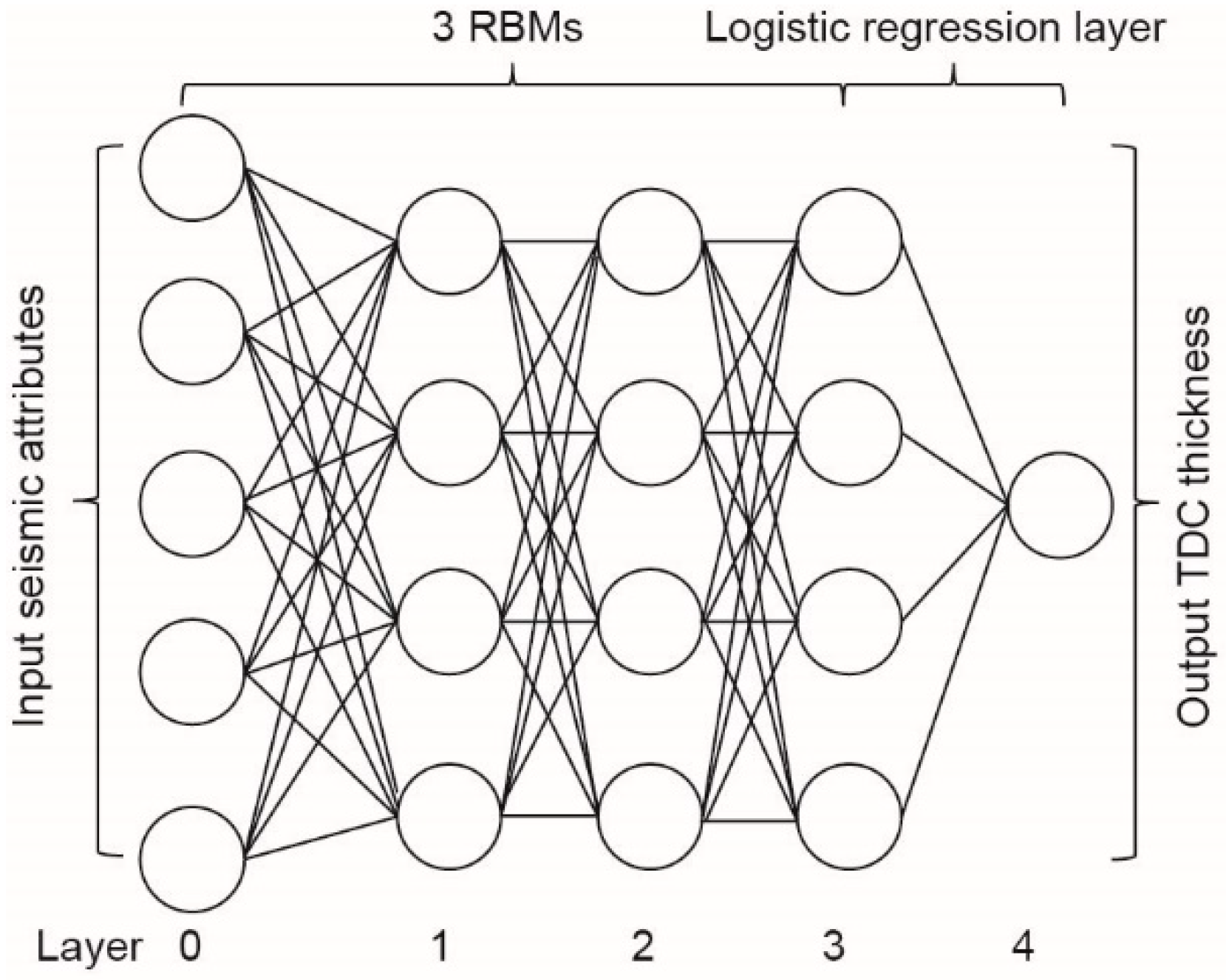
The DBN is a feedforward neural network with many hidden layers, allowing the DBN to be robust in modeling the complicated relationship among the data [19,20,21]. As an instance, Figure 2 shows TDC thickness prediction with the DBN and seismic attributes. The first RBM maps input seismic attributes into the 0th layer to form the first-layer feature. The training manner in this procedure is the same as the above-mentioned RBM. Then, subsequent layers of RBM are trained via the output of its previous layer. The features of the last RBM are the learned features of the whole training system. Finally, a logistic regression layer is added to the end of featured learning systems. It is used to fine-tune the whole pertained network to integrate the layers of neural networks and perform thickness prediction by utilizing the learned features.

3. Synthetic Example

3.1. Synthetic Data Preparing

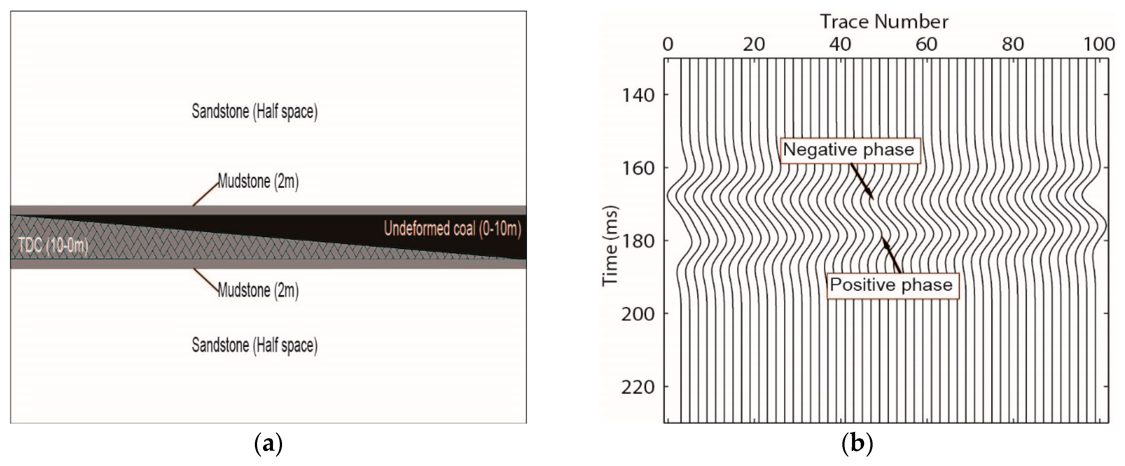
To study the applicability of DBN on the TDC thickness prediction, a DBN prediction model with the input of seismic attributes was built from a synthetic seismic section. Firstly, we developed a geological section referencing the actual geological characteristics of an actual coalbed and its nearby strata, as shown in Figure 3a. The length of the section was 1 km. From left to right, the thickness of TDC (P-velocity = 1.5 km/s) decreased from 10 m to 0 m; in contrast, the thickness of undeformed coal (P-velocity = 2.4 km/s) increased from 0 m to 10 m. The direct roof and floor were 2 m thick mudstone (P-velocity = 3.2 km/s), beyond which and extended to the half-space were sandstone (P-velocity = 3.6 km/s). By calculating the reflectivities at all P-velocity interfaces with 10 m lateral space and convolving the reflectivities with a 50 Hz Ricker wavelet, we achieved a synthetic seismic section (98 seismic traces) of the corresponding geological section, as shown in Figure 3b.
As shown in Figure 3a, the thickness of the coal bed was constant, and about a quarter of the seismic wavelength (~10 m). The top and the bottom interfaces of the coalbed were probably related to different seismic phases, i.e., the negative phase and the positive phase, as shown in Figure 3b. Since TDC’s P-velocity was much smaller than the undeformed coal, the two-way-time (TWT) of a seismic wave traveling in the coalbed differed from trace to trace. The TWT increased with the thickness of TDC. The TWT of the location with thin TDC was small. Consequently, the lower positive phase was dipping from the right side to the left side, as shown in Figure 3b.
As the coalbed was thick and the TDC spread out at the bottom of the coalbed, the lower positive phase was probably related to the TDC more directly than the upper negative phase. In the seismic industry, amplitude, frequency, structure, and spectral-decomposition (SD) attributes are the most conventional and easily accessible seismic attributes [11,16]. Through extracting the attributes from the positive phase, we built a DBN model to forecast the TDC thickness. The attributes used here were curvature (Attr1), dominant frequency (Attr2), instantaneous frequency (Attr3), sweetness (Attr4), 30 Hz SD (Attr5), 50 Hz SD (Attr6), 60 Hz SD (Attr7), 70 Hz SD (Attr8), and 90 Hz SD (Attr9), instantaneous amplitude (Attr10), and bandwidth (Attr11) [8,9,11].

3.2. Dimensional Reduction and TDC Prediction

The typical characteristics of seismic attributes are the high dimensionality and the possible correlations among them, which are the main obstacles in the practical application. For the synthetic example, we calculated the correlation coefficient matrix of seismic attributes, as shown in Table 1. Some similarities were observed between the seismic attributes. We used PCA algorithms to reduce the dimension of input seismic attributes. The characteristics of eigenvalues and PCs are shown in Table 2. For the first PC, the variance contribution was 0.937 (accounting for 93.7% variation); for the last PC, the variance contribution was 0 (accounting for 0% variation). The cumulative variance contribution of the first three PCs was greater than 0.85 (0.998), i.e., the first three PCs could represent the most information variations of input seismic attributes.
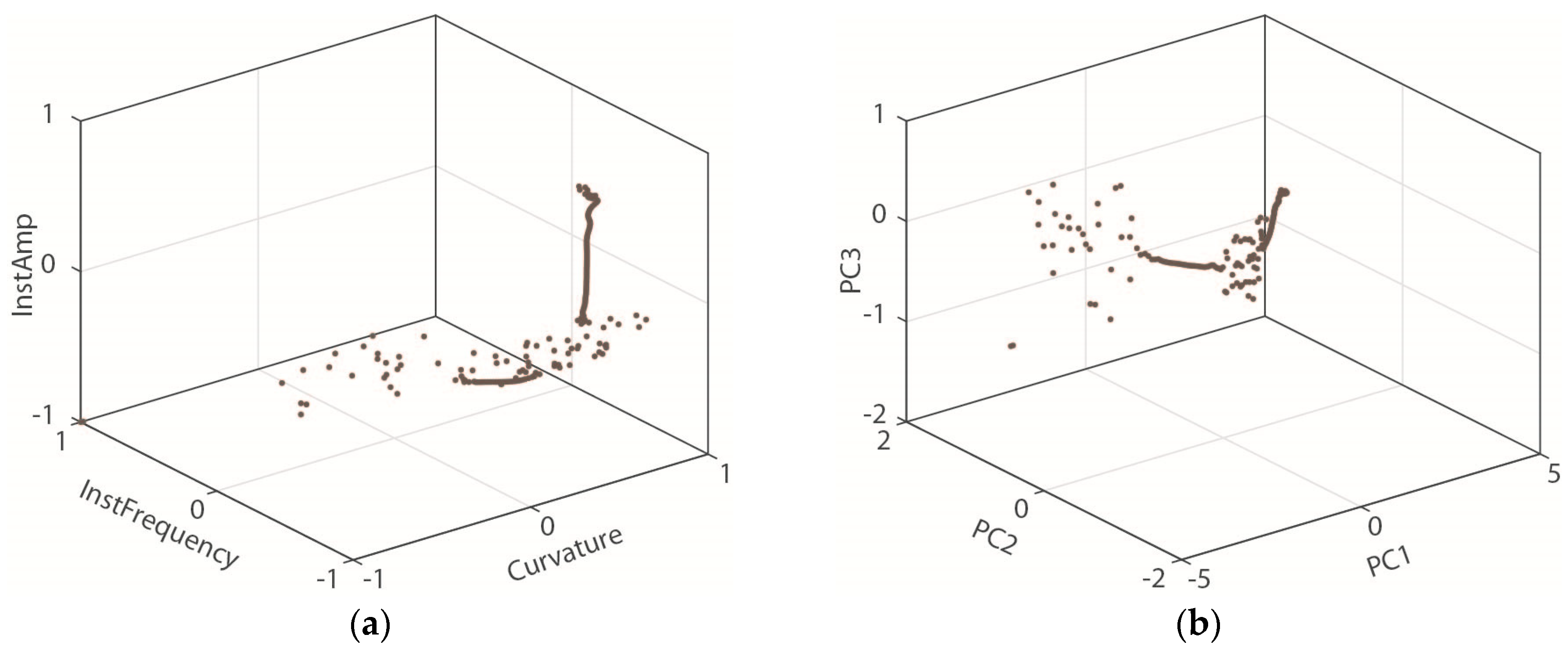
Since the curvature, instantaneous frequency, and instantaneous amplitude are the most used seismic attributes, a cross plot of them (Figure 4a) was created and compared with that of the first three PCs (Figure 4b), respectively. As could be seen, the cross plot of curvature, instantaneous frequency, and instantaneous amplitude was poorly separated, whereas the cross plot of the first three PCs was well separated. After PCA, the probably correlated seismic attributes were transformed into linearly independent PCs, which gave the preferred input of the DBN prediction model.

3.3. Prediction Comparison

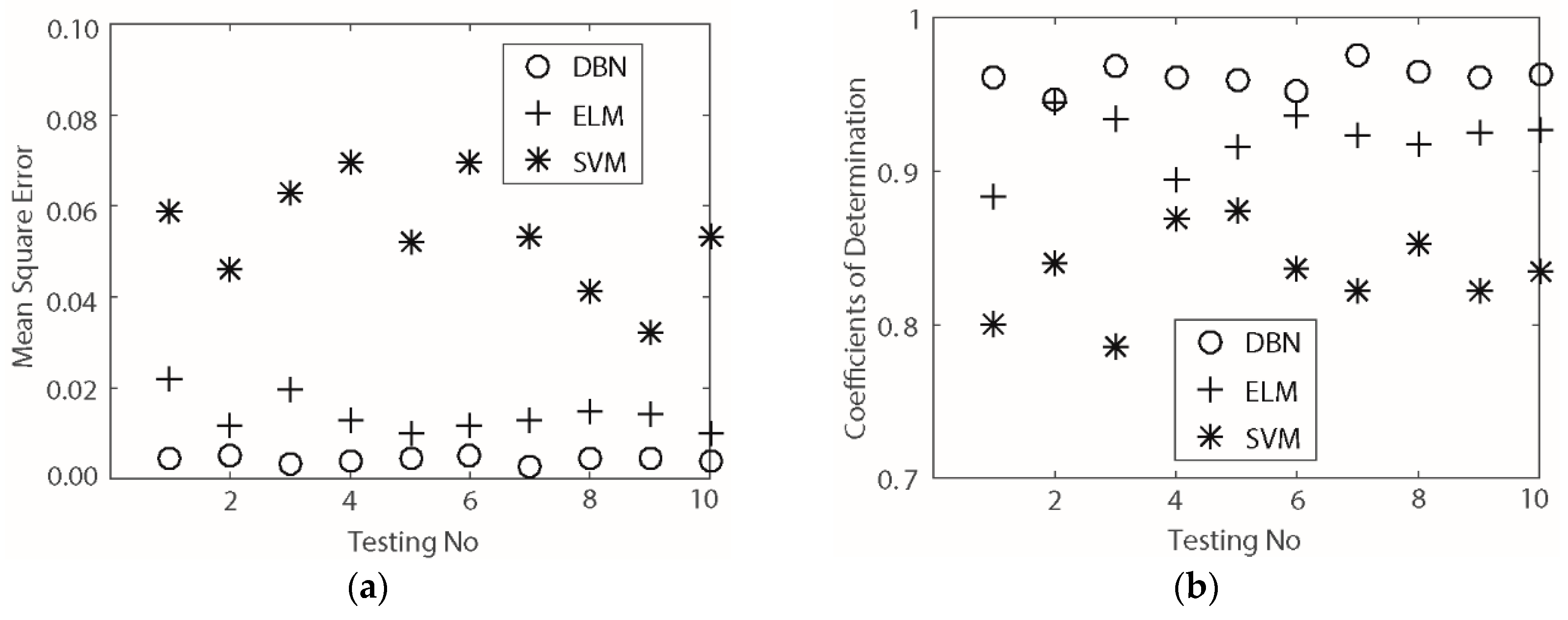
In the literature, the methods, such as SVM and ELM, have been used to predict the TDC thickness and have achieved satisfactory prediction results [11,16]. To verify the forecast performance of DBN, we compared the forecast thickness of the DBN model with the SVM model and the ELM model [11,16,27]. For the SVM model, we used the libsvm toolbox [28] to train and predict the thickness, where the kernel function was radial basis function, the search space of parameter c and g was (–30, 30), and the step size was 0.5. For the ELM model, we used the sigmoid function as the activation function and set the hidden node to 10. To maintain consistency, we randomly separated the seismic traces (98 in total) into a training data set with 68 traces and a testing data set with 30 traces and used the same training set and testing set for all predicting models. To ensure the comparison reliability, we repeated each experiment ten times and plotted the mean square errors, as well as the corresponding determination coefficients, in Figure 5.
Compared with the ELM model and SVM model, the DBN model showed the best accuracy and stability on the prediction of TDC thickness, and it was chosen as the preferred model for the following experiments.

4. Case Study

4.1. General Settings

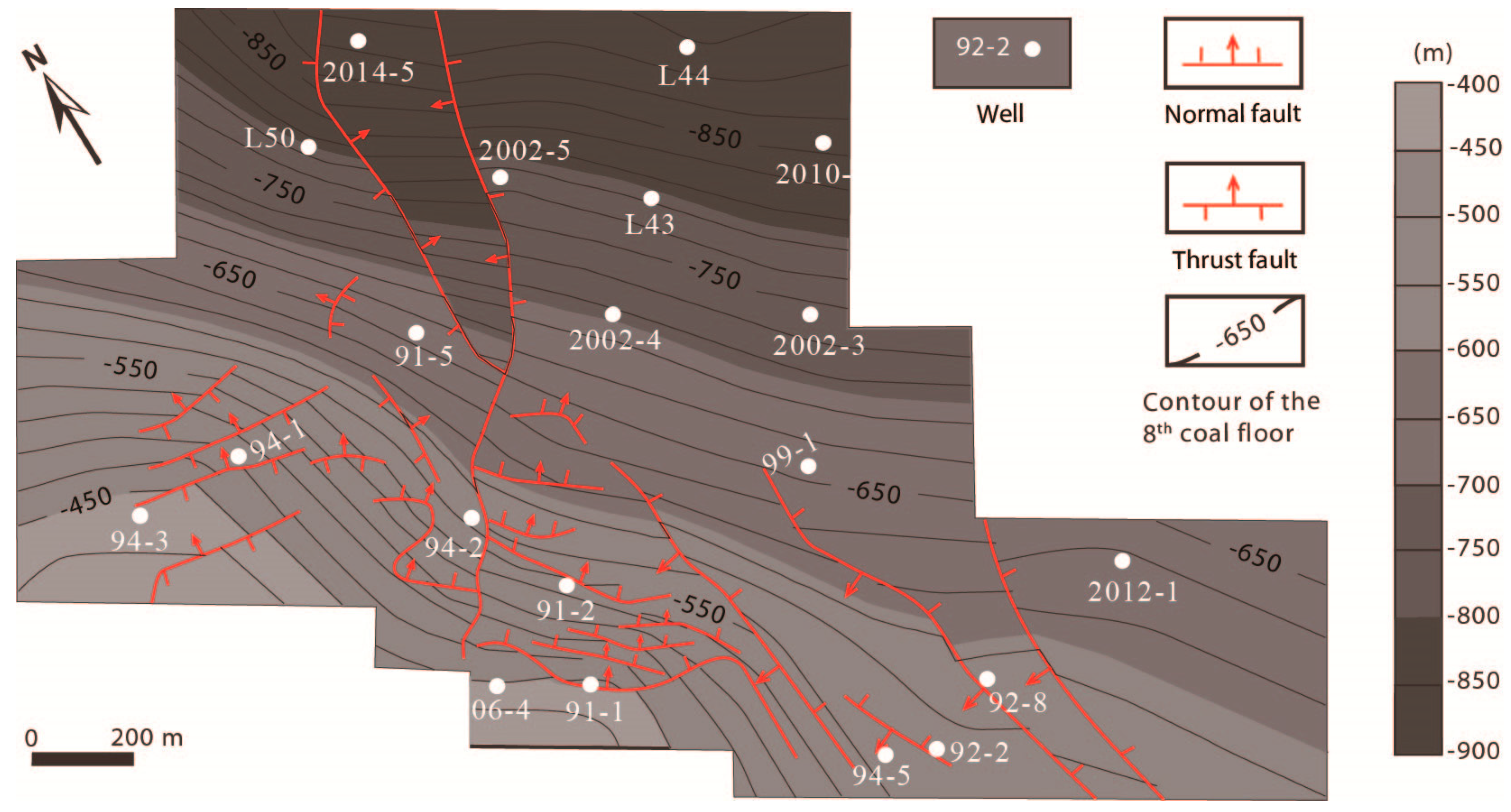
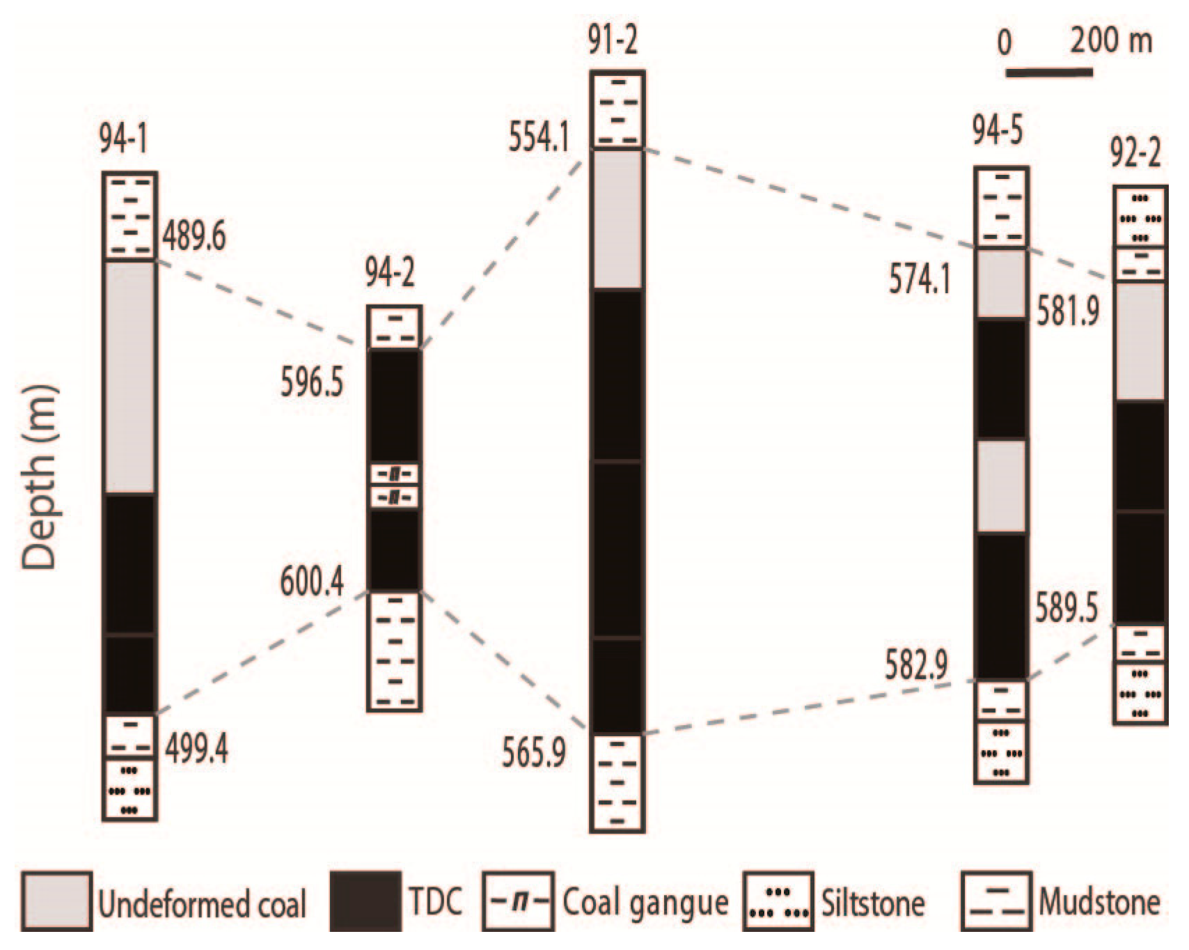
The Luling coal mine is a gas-outburst prone mine, located in the north of Anhui province, eastern China. In the study area, 20 pre-drilled wells have confirmed the existence of coalbed No. 8. According to the wells, the burial depth of coalbed No. 8 is between 448.6 m and 930.7 m, as shown in Table 3. During the past geological periods, including the Indosinian, the Yanshanian, and the Himalayanian, the coalfield of this mine experienced complex tectonic movements and formed complex tectonic structures [15,29]. Based on the structural interpretation of the 3D seismic volume acquired earlier, the study area is a monocline structure dipping toward the NE direction, as shown in Figure 6. From the bottom to the top, the elevation of coalbed No. 8 gradually increases from −400 m to −900 m, indicating the gradual increase of burial depth as the surface elevation in the area is relatively flat (~30 m). Besides, three sets of tectonic faults extend along the EW, the NS, and the NNW directions in the study area. Because of the previous tectonic movements, coalbed No. 8 has developed considerable TDC, which are mostly identified at the bottom of the coalbed, as shown in Figure 7 [15,29].

4.2. Cross-Validation

On the pre-drilled 20 vertical wells in the study area, density, gamma-ray, and electricity logs were conducted. By analyzing these logs, as did by Chen et al. [29], we were able to identify the TDC and the thickness for every individual well. As is shown in Table 3 and Figure 7, the thickest TDC was 11.6 m, the thinnest TDC was 3.8 m, and the mean was 6.7 m. Besides, the TDC thickness had a positive correlation with the buried depth of coalbed No. 8, which is the typical development characteristic of TDC in the study area [29].
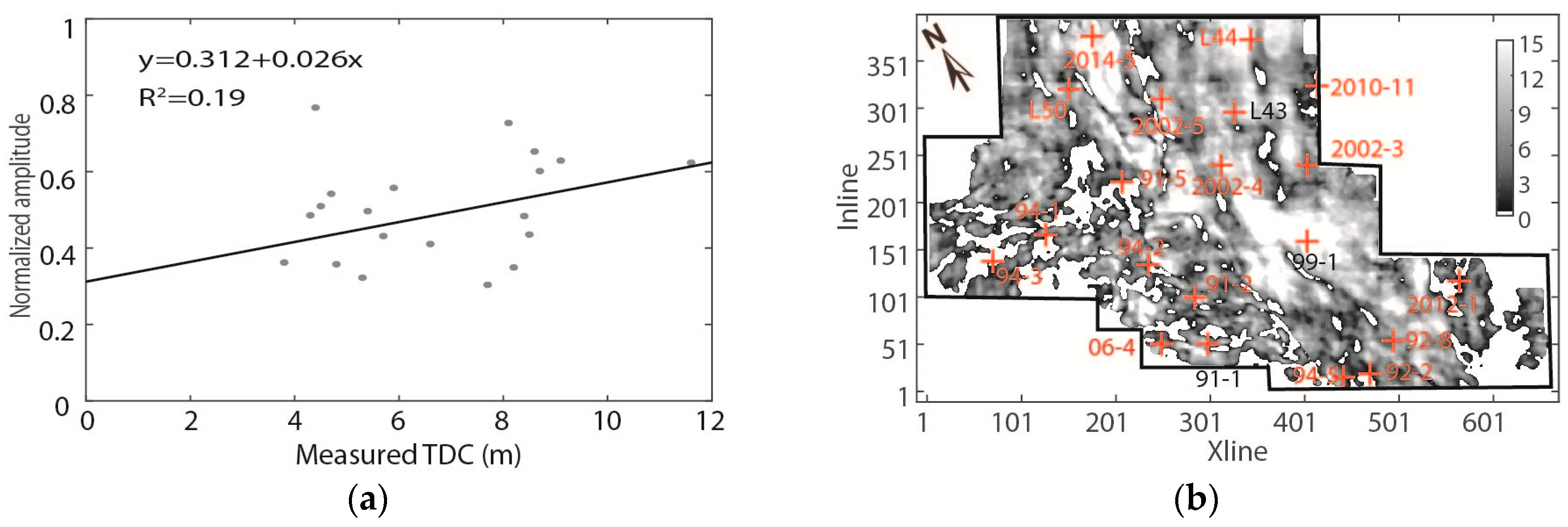
It is well known that seismic amplitude is positively related to the acoustic impedance contrast, and strong impedance contrast exists on the coalbed’s roof and floor. Therefore, it is theoretically possible to estimate TDC distribution in a coalbed qualitatively using seismic amplitude. Here, the stacked 3D seismic volume was gridded by 5 m × 5 m × 1 ms, and every individual well was coinciding with an individual seismic trace geographically. We extracted instantaneous amplitudes of near-well traces and cross plotted them with the measured TDC thickness, as shown in Figure 8a. The amplitude was associated with TDC thickness, but the link was weak. By predicting with the fitted equation and amplitude, we achieved a TDC distribution of coalbed No. 8, as shown in Figure 8b. As the distribution was less accurate, it was necessary to adopt a method with multiple seismic attributes to predict the TDC thickness of coalbed No. 8.
Although the initial DBN prediction model demonstrated its ability to the prediction of the TDC thickness with the input of synthetic seismic data, it was not convincible to use it with real seismic data. The reason was that the synthetic data and the real seismic data probably differ in signal-to-noise ratio, frequency, phase, and bandwidth. Therefore, we used near-well traces to evaluate the applicability of the DBN prediction model, where we knew the true TDC thickness and real seismic attributes. The seismic attributes used here were the same as the synthetic data.
Although every individual well had a near-well trace, the data set with these 20 near-well traces were not larger enough to guarantee the training of a reliable DBN prediction model. Assuming the geology near the wells was stable in the lateral direction within small spatial deviation, we could treat the traces as the near-well traces if they were within 25 m nearby zones from the wells. The TDC thicknesses of these near-well traces were included for the prediction of the TDC thicknesses of their parental wells. As a result, 1359 traces were used to validate the DBN prediction model.
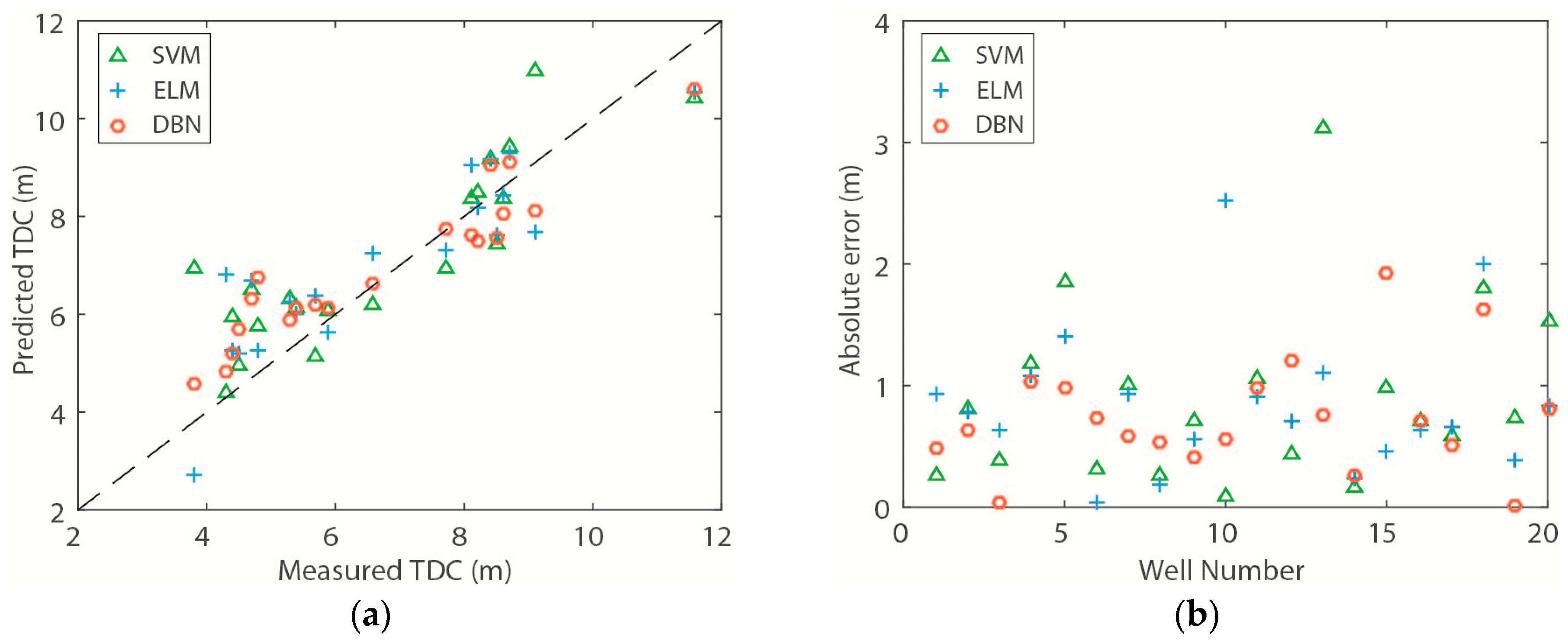
During the prediction, we extracted seismic attributes as we did in Section 3.1 and computed their principal components (PCs). Similar to the synthetic example, the seismic attributes here were correlated with each other, and the first three PCs accounted for over 85% variance (93.8%), as shown in Table 4 and Table 5. Then, we used the first three PCs of near-well traces to form the training set and the testing set. The testing dataset included the near-well traces of a chosen well, and the training set included the near-well traces of the rest 19 wells. After repeating this classical cross-validation for every single well, we had the predicted TDC thickness. In addition, we compared the predicted thicknesses of the DBN model with the real thicknesses, as well as the forecasted thicknesses of the SVM and ELM models, to evaluate the forecasting accuracy and reliability, as shown in Table 6 and Figure 9.

4.3. Prediction

In general, the predicted TDC thicknesses using the near-well traces are accurate and reliable. As is shown, the SVM model gave the poorest results with an average error of 0.90 m, and the ELM model gave the second poorest results with an average error of 0.85 m. In comparison, the DBN model gave the best results with an average error of 0.74 m.
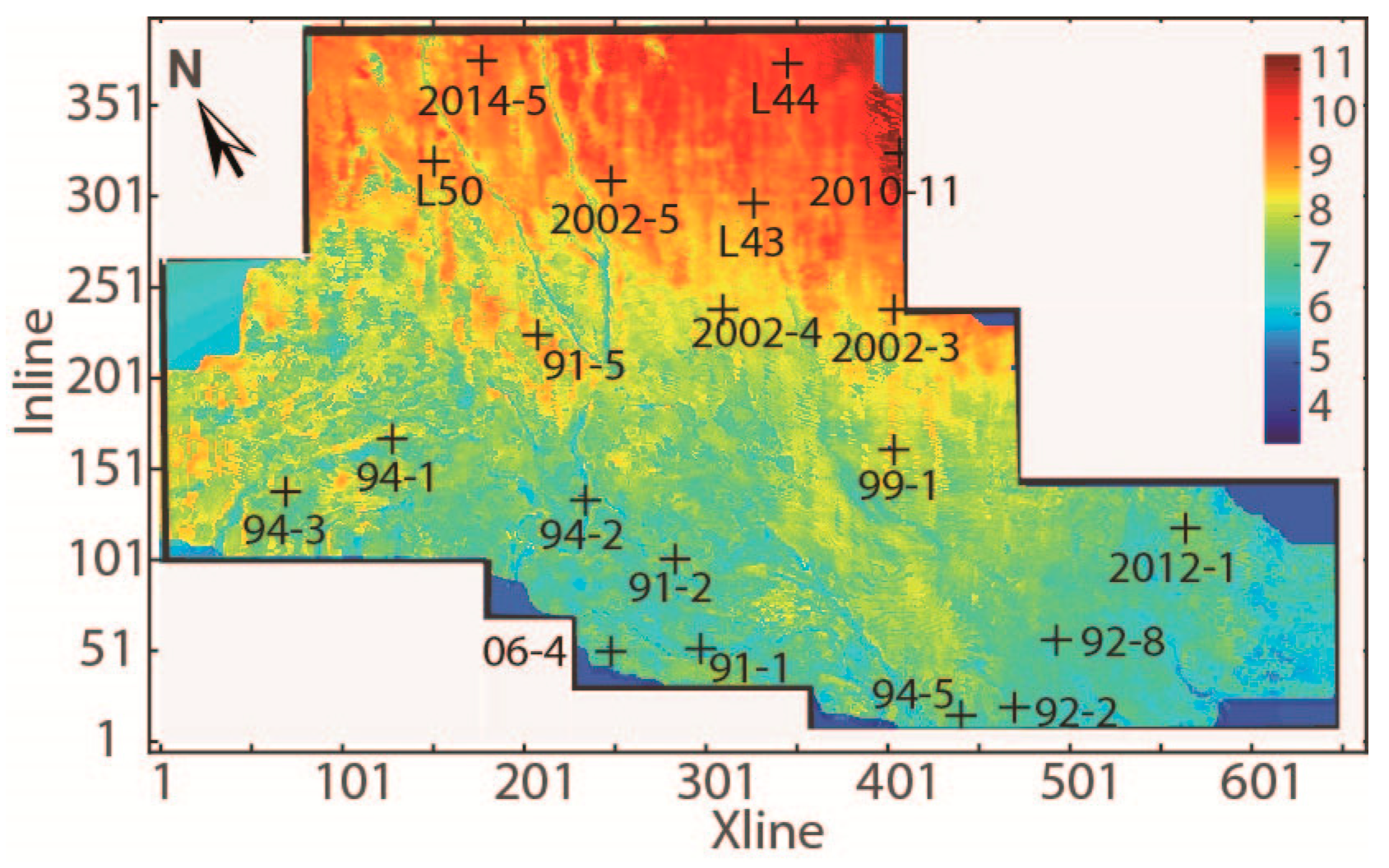
Since the DBN model was the best in the TDC-thickness prediction, we used the first three PCs from all near-well traces of the 20 wells to form the training set and use the trained DBN model to predict the TDC thickness of coalbed No. 8 in the study area. Again, we repeated the training and predicting ten times and used the mean as the final TDC-thickness prediction, as shown in Figure 10. The thickest TDC was in the NE corner, where the burial depth was the deepest; the medium-thick TDC was in the middle area, where the burial depth was the medium; the thinnest TDC was in the SE corner, where the burial depth was shallow.

4.4. Discussions

4.4.1. Influences of Burial Depth and Coalbed Thickness

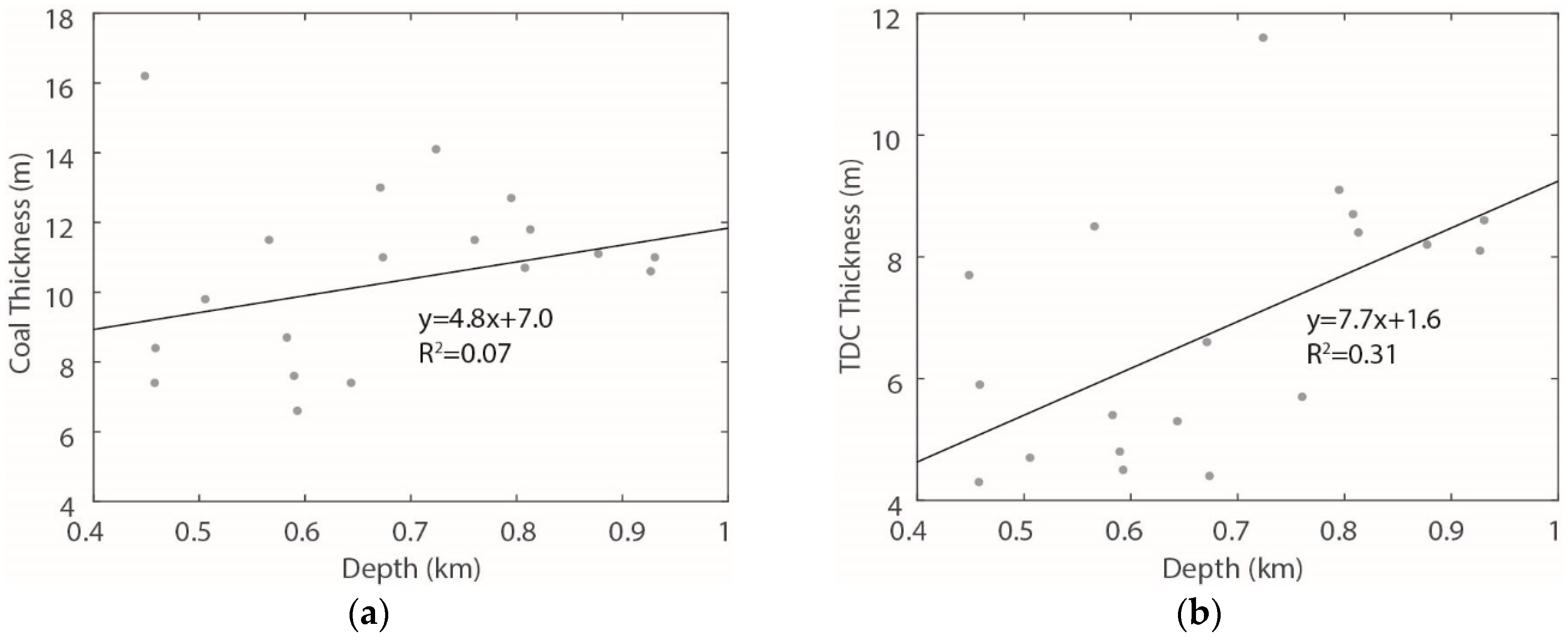
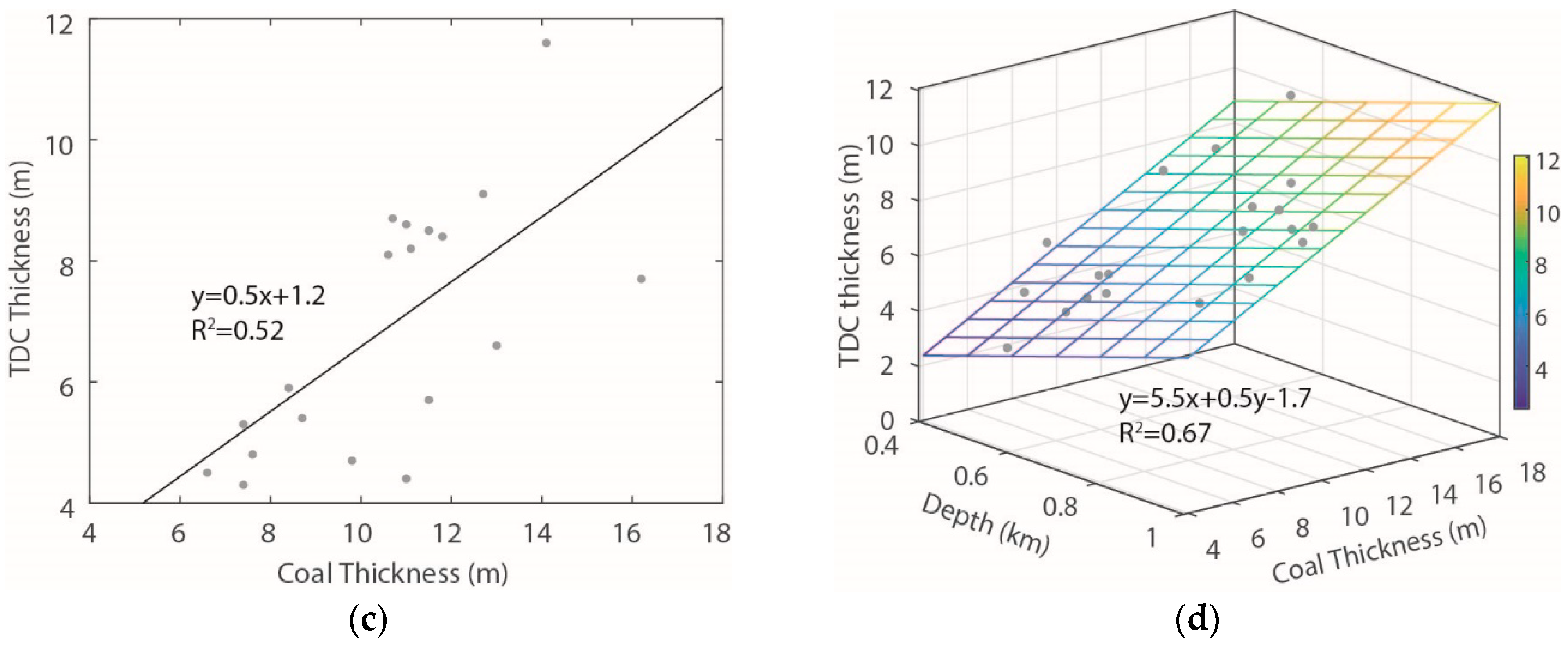
To understand the influence factors of TDC thickness, we analyzed the association among the burial depth, TDC thickness, and coalbed thickness, as shown in Figure 11. All the data used here were from the measured results from the 20 pre-drilled wells. The coalbed thickness was mainly related to the depositional conditions and might have less to do with the burial depth. The burial depth only accounted for a 7% variation of coalbed thickness (R2 = 0.07), as shown in Figure 11a, which was consistent with the general understanding of the influence factors of coalbed thickness. As observed by Jiang et al. [15], TDC thickness was associated with the burial depth and coalbed thickness. In our experiments, the burial depth accounted for a 31% variation of TDC thickness (R2 = 0.31), and the coalbed thickness accounted for a 52% variation of TDC thickness (R2 = 0.52), as shown in Figure 11b,c. Considering the burial depth and coalbed thickness simultaneously, they accounted for a 67% variation of TDC thickness (R2 = 0.67), as shown in Figure 11d.
As the revealed characteristics of borehole data, the predicted TDC thickness of the study area from the seismic attributes also showed a similar correlation between the burial depth and the TDC thickness. As shown in Figure 10 and Figure 6, the thickest TDC was in the NE part, where the burial depth was deepest; the thinnest TDC was in the SW part, where the burial depth was shallowest; the medium-thick TDC was in the middle, where the burial depth was medium. Clearly, the predicted TDC thickness in the study area was positively correlated with the burial depth, as indicated by Chen et al. and Jiang et al. [15,29].

4.4.2. Influences of Fault Development

Besides the burial depth and coalbed thickness, the structural deformation related to the tectonic movement was another main factor influencing TDC thickness. The stronger the tectonically structural development was, the thicker was the TDC thickness. In the Huaibei coalfield, the faults are the main indicator of tectonically structural development [15]. The dense the fault distribution was, the higher was the tectonically structural development.
The fault distribution, as shown in Figure 6, was interpreted from the 3D seismic volume. Because of the influence of seismic resolution, the reliability of interpreted faults for the deep burial coalbed is lower than the shallow burial coalbed [30]. In this case, the NE part was much deeper than the SW part. Considering the consistency of seismic resolution, we only considered the shallow area during the comparison, i.e., the SW part.
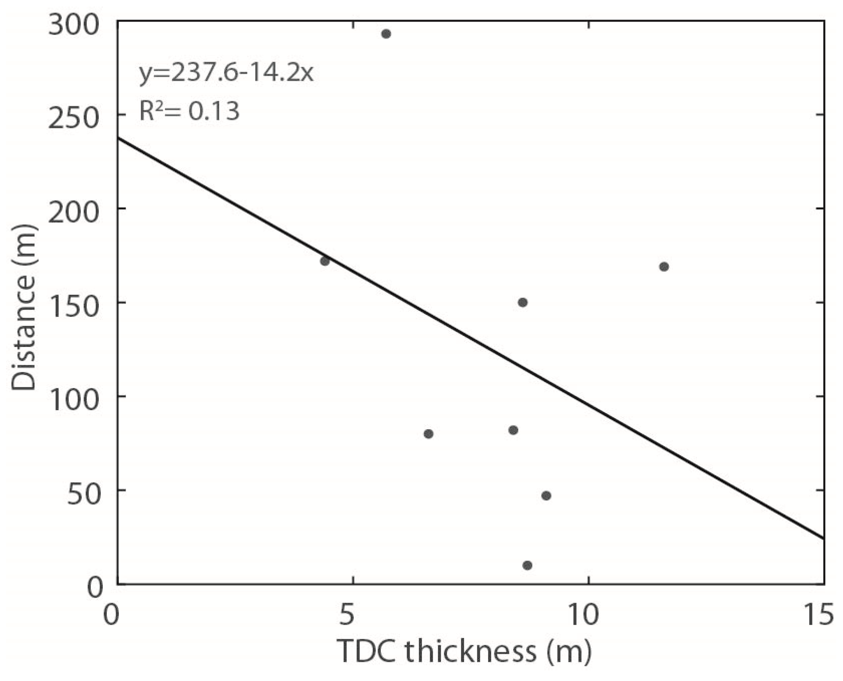
As is shown, the fault density was high at the SW corner and was low at the SE corner. In Figure 10, the predicted TDC thickness at the SW corner was higher than the SE corner, but the SW corner was almost 100 m shallower than the SE corner. We measured the distance from well to its nearest fault, and cross plotted the distance with the TDC thickness of parental well. The TDC thickness was negatively correlated with the distance, as shown in Figure 12. This might well explain why combing burial depth and coalbed thickness only accounted for 67% variance of the TDC thickness, as shown in Section 4.4.1, meaning that fault development was also an important influence factor of the TDC thickness in the study area.

4.4.3. Prediction Comparison

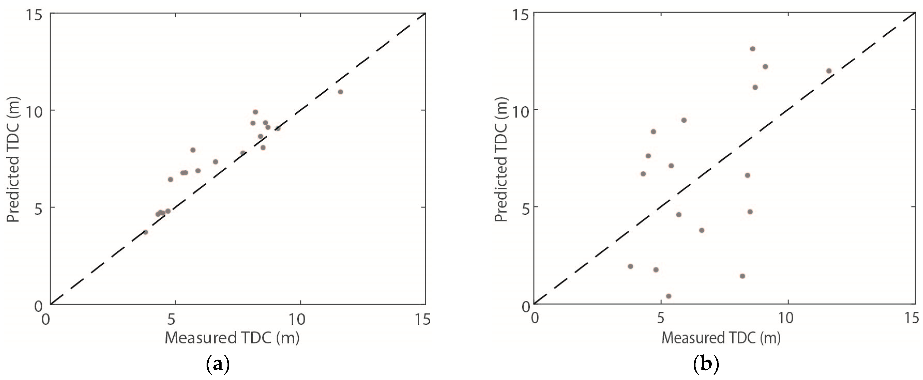
We predicted TDC distributions with a DBN model and the instantaneous amplitude, as shown in Figure 8b and Figure 10. They were far different from each other. To compare their prediction accuracy, we cross plotted the measured and predicted TDC thickness at well locations in Figure 13. As is shown, the scattering points of Figure 13a were near the diagonal with a small deviation (0.73 m on average), while the scattering points of Figure 13b were far from the diagonal with a large deviation (4 m on average). In addition, the predicted distribution with a DBN model followed the regional characteristics of TDC development, i.e., TDC thickness was associated with burial depth, coalbed thickness, and structural development. In contrast, the predicted distribution with instantaneous amplitude had a weak link to the regional characteristics of TDC development. Across the right side of the study area, the predicted TDC thickness was mostly thick (>6.7 m).

5. Conclusions

In this paper, we proposed a prediction method for the TDC thickness of coalbed with a DBN model and PCA. Based on the testing results of a synthetic example and a case study from an operational coal mine, we achieved the following observations and recommendations:
(1)
The predicted TDC thicknesses with SVM, ELM, and DBN models were accurate and stable, while the DBN model provided the best results considering the prediction accuracy and stability. However, it is worthy of further studies of this model on the TDC thickness prediction in some other areas.
(2)
Both synthetic and measured seismic attributes had more or less correlation with each other. PCA could transform the high dimensional seismic attributes into low dimensional PCs and simplify the complexity of TDC-thickness prediction.
(3)
The burial depth, coalbed thickness, and fault development were the main influence factors for the TDC thickness in the study area. This observation was consistent with the known regional characteristics of TDC development.

Author Contributions

Conceived and designed the algorithms, X.W. and T.C.; Performed the algorithms, X.W., T.C. and H.X.; Analyzed the data, X.W., T.C. and H.X.; Wrote the paper, X.W. and T.C. All authors have read and agreed to the published version of the manuscript.

Funding

This research was funded by the National Natural Science Foundation of China, grant number 41704115 and No. 41774128, the Natural Science Foundation of Jiangsu Province, grant number BK20170273, and A Project Funded by the Priority Academic Program Development of Jiangsu Higher Education Institutions (PAPD).

Conflicts of Interest

The authors declare no conflict of interest.

References

  1. Cao, Y.X.; Davis, A.; Liu, R.X.; Liu, X.W.; Zhang, Y.G. The influence of tectonic deformation on some geochemical properties of coal—A possible indicator of outburst potential. Int. J. Coal Geol. 2003, 53, 69–79. [Google Scholar] [CrossRef]
  2. Li, M.; Jiang, B.; Lin, S.; Wang, J.; Ji, M.; Qu, Z. Tectonically deformed coal types and pore structures in Puhe and Shanchahe coal mines in western Guizhou. Min. Sci. Technol. 2011, 21, 353–357. [Google Scholar] [CrossRef]
  3. Li, H.Y. Major and minor structural features of a bedding shear zone along a coal seam and related gas outburst, Pingdingshan coalfield, northern China. Int. J. Coal Geol. 2001, 47, 101–113. [Google Scholar] [CrossRef]
  4. Li, H.Y.; Ogawa, Y.; Shimada, S. Mechanism of methane flow through sheared coals and its role on methane recovery. Fuel 2003, 82, 1271–1279. [Google Scholar] [CrossRef]
  5. Ju, Y.W.; Li, X.S. New research progress on the ultrastructure of tectonically deformed coals. Prog. Nat. Sci. Mater. 2009, 19, 1455–1466. [Google Scholar] [CrossRef]
  6. Yao, J.-P.; Sima, L.-Q.; Zhang, Y.-G. Quantitative identification of deformed coals by geophysical logging. Meitan Xuebao/J. China Coal Soc. 2011, 36 (Suppl. 1), 94–98. [Google Scholar]
  7. Xue, G.; Liu, H.; Li, W. Deformed coal types and pore characteristics in Hancheng coalmines in Eastern Weibei coalfields. Int. J. Min. Sci. Technol. 2012, 22, 681–686. [Google Scholar] [CrossRef]
  8. Bunt, R.J.W. The use of seismic attributes for fan and reservoir definition in the Sea Lion Field, North Falkland Basin. Pet. Geosci. 2015, 21, 137–149. [Google Scholar] [CrossRef]
  9. Hart, B.S. Channel detection in 3-D seismic data using sweetness. AAPG Bull. 2008, 92, 733–742. [Google Scholar] [CrossRef]
  10. Jahan, I.; Castagna, J.; Murphy, M.; Kayali, M.A. Fault detection using principal component analysis of seismic attributes in the Bakken Formation, Williston Basin, North Dakota, USA. Interpret. J. Sub 2017, 5, T361–T372. [Google Scholar] [CrossRef]
  11. Wang, X.; Li, Y.; Chen, T.J.; Yan, Q.Y.; Ma, L. Quantitative thickness prediction of tectonically deformed coal using Extreme Learning Machine and Principal Component Analysis: A case study. Comput. Geosci. 2017, 101, 38–47. [Google Scholar] [CrossRef]
  12. Lu, J.; Wang, Y.; Chen, J.Y. Detection of Tectonically Deformed Coal Using Model-Based Joint Inversion of Multi-Component Seismic Data. Energies 2018, 11, 829. [Google Scholar] [CrossRef]
  13. Teng, J.; Yao, Y.B.; Liu, D.M.; Cai, Y.D. Evaluation of coal texture distributions in the southern Qinshui basin, North China: Investigation by a multiple geophysical logging method. Int. J. Coal Geol. 2015, 140, 9–22. [Google Scholar] [CrossRef]
  14. Wu, H.B.; Dong, S.H.; Huang, Y.P.; Chen, G.W.; Wang, H.L. A Method for Coal Structure Division Based on Avo Simultaneous Inversion. J. Seism. Explor. 2015, 24, 365–377. [Google Scholar]
  15. Jiang, B.; Qu, Z.H.; Wang, G.G.X.; Li, M. Effects of structural deformation on formation of coalbed methane reservoirs in Huaibei coalfield, China. Int. J. Coal Geol. 2010, 82, 175–183. [Google Scholar] [CrossRef]
  16. Chen, T.-J.; Wang, X.; Guan, Y.-W. Quantitative prediction of tectonic coal seam thickness using support vector regression and seismic attributes. Meitan Xuebao/J. China Coal Soc. 2015, 40, 1103–1108. [Google Scholar]
  17. Wang, X.; Chen, T. Quantitative prediction of tectonic coal thickness based on FNN and seismic attributes. J. Inf. Comput. Sci. 2014, 11, 3653–3662. [Google Scholar] [CrossRef]
  18. Hinton, G.E.; Osindero, S.; Teh, Y.W. A fast learning algorithm for deep belief nets. Neural Comput. 2006, 18, 1527–1554. [Google Scholar] [CrossRef]
  19. Liu, W.B.; Wang, Z.D.; Liu, X.H.; Zengb, N.Y.; Liu, Y.R.; Alsaadi, F.E. A survey of deep neural network architectures and their applications. Neurocomputing 2017, 234, 11–26. [Google Scholar] [CrossRef]
  20. Chen, Y.S.; Zhao, X.; Jia, X.P. Spectral-Spatial Classification of Hyperspectral Data Based on Deep Belief Network. IEEE J. Stars 2015, 8, 2381–2392. [Google Scholar] [CrossRef]
  21. Sarikaya, R.; Hinton, G.E.; Deoras, A. Application of Deep Belief Networks for Natural Language Understanding. IEEE-ACM Trans. Audio Speech 2014, 22, 778–784. [Google Scholar] [CrossRef] [Green Version]
  22. Ringner, M. What is principal component analysis? Nat. Biotechnol. 2008, 26, 303–304. [Google Scholar] [CrossRef] [PubMed]
  23. Hu, S.; Zhao, W.; Xu, Z.; Zeng, H.; Fu, Q.; Jiang, L.; Shi, S.; Wang, Z.; Liu, W. Applying principal component analysis to seismic attributes for interpretation of evaporite facies: Lower Triassic Jialingjiang Formation, Sichuan Basin, China. Interpret. A J. Subsurf. Charact. 2017, 5, T461–T475. [Google Scholar] [CrossRef]
  24. Barrash, W.; Morin, R.H. Recognition of units in coarse, unconsolidated braided-stream deposits from geophysical log data with principal components analysis. Geology 1997, 25, 687–690. [Google Scholar] [CrossRef]
  25. Jolliffe, I.T. Principal Component Analysis, 2nd ed.; Springer: New York, NY, USA, 2002; pp. 44–46. [Google Scholar]
  26. Hinton, G.E.; Salakhutdinov, R.R. Reducing the dimensionality of data with neural networks. Science 2006, 313, 504–507. [Google Scholar] [CrossRef] [Green Version]
  27. Huang, G.B.; Zhu, Q.Y.; Siew, C.K. Extreme learning machine: Theory and applications. Neurocomputing 2006, 70, 489–501. [Google Scholar] [CrossRef]
  28. Chang, C.-C.; Lin, C.-J. LIBSVM: A library for support vector machines. ACM Trans. Intell. Syst. Technol. 2011, 2, 1–27. [Google Scholar] [CrossRef]
  29. Chen, T.J.; Ma, G.D.; Wang, X.; Cui, R.F. Deformation Degree Estimate for Coal Seam using Well Logs as Input: A Case Study. J. Environ. Eng. Geophys. 2018, 23, 89–101. [Google Scholar]
  30. Sheriff, R.E. Encyclopedic Dictionary of Applied Geophysics, 4th ed.; Society of Exploration Geophysicists: Tulsa, OK, USA, 2002. [Google Scholar]
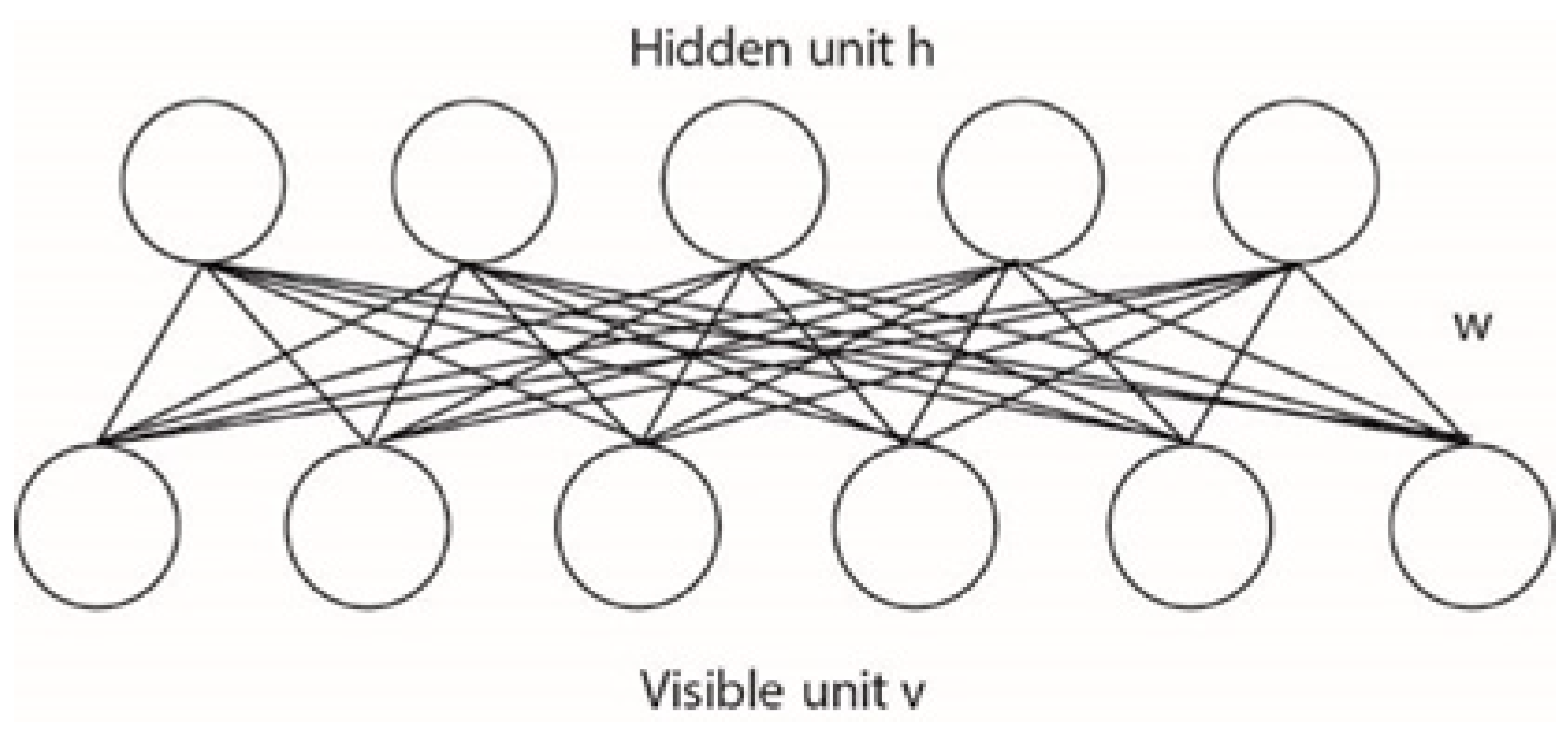
Figure 1. Schematic illustration of a restricted Boltzmann machine (RBM).
Energies 13 01169 g001
Figure 2. Schematic deep belief network (DBN) model for the tectonically deformed coal (TDC) thickness prediction.
Energies 13 01169 g002
Figure 3. A geological coalbed model (a), and its corresponding synthetic seismic section (b).
Energies 13 01169 g003
Figure 4. The cross plots of the seismic attributes (a) and the principal components (PCs) (b).
Energies 13 01169 g004
Figure 5. The predicted mean square errors (a) and determination coefficients (b) among the DBN, extreme learning machine (ELM), and support vector machine (SVM) models.
Energies 13 01169 g005
Figure 6. An overview map of No. 8 coal’s elevation.
Energies 13 01169 g006
Figure 7. Geological section across wells of 94-1, 94-2, 91-2, 94-5, and 92-2.
Energies 13 01169 g007
Figure 8. Cross plot between measured TDC and normalized amplitude (a), and amplitude predicted TDC thickness in meters (b).
Energies 13 01169 g008
Figure 9. Comparisons of the measured and predicted TDC thicknesses (a) and the TDC-thickness errors (b) after classical cross-validation.
Energies 13 01169 g009
Figure 10. The predicted TDC thickness in meters of coalbed No. 8 in the study area. The “+” markers indicate the well locations, and the labels beside the markers are well names.
Energies 13 01169 g010
Figure 11. Cross plots of coal thickness vs. depth (a), TDC thickness vs. depth (b), TDC thickness vs. coal thickness (c), and TDC thickness vs. depth and coal thickness (d).
Energies 13 01169 g011aEnergies 13 01169 g011b
Figure 12. Cross plots of TDC thickness vs. distance to well’s nearest fault.
Energies 13 01169 g012
Figure 13. Cross plots of measured TDC thickness vs. predicted TDC thickness with a DBN model (a), and measured TDC thickness vs. predicted TDC thickness with instantaneous amplitude (b).
Energies 13 01169 g013
Table 1. Correlation coefficient matrix.
Attr1Attr2Attr3Attr4Attr5Attr6Attr7Attr8Attr9Attr10Attr11
Attr11.00 −0.18 −0.17 0.09 0.10 0.10 0.09 0.09 0.08 0.08 0.15
Attr2−0.18 1.00 0.99 −0.76 −0.78 −0.78 −0.77 −0.77 −0.75 −0.75 −0.83
Attr3−0.17 0.99 1.00 −0.84 −0.85 −0.85 −0.85 −0.84 −0.83 −0.83 −0.90
Attr40.09 −0.76 −0.84 1.00 1.00 1.00 1.00 1.00 1.00 1.00 0.98
Attr50.10 −0.78 −0.85 1.00 1.00 1.00 1.00 1.00 1.00 1.00 0.98
Attr60.10 −0.78 −0.85 1.00 1.00 1.00 1.00 1.00 1.00 1.00 0.98
Attr70.09 −0.77 −0.85 1.00 1.00 1.00 1.00 1.00 1.00 1.00 0.98
Attr80.09 −0.77 −0.84 1.00 1.00 1.00 1.00 1.00 1.00 1.00 0.98
Attr90.08 −0.75 −0.83 1.00 1.00 1.00 1.00 1.00 1.00 1.00 0.98
Attr100.08 −0.75 −0.83 1.00 1.00 1.00 1.00 1.00 1.00 1.00 0.98
Attr110.15 −0.83 −0.90 0.98 0.98 0.98 0.98 0.98 0.98 0.98 1.00
Table 2. The characteristics of eigenvalues and principal components (PCs).
PCsEigenvaluesVariance ContributionsCumulative Contributions
PC13.332 0.937 0.937
PC20.177 0.050 0.986
PC30.042 0.012 0.998
PC40.006 0.002 1.000
Table 3. Well-logging measured TDC thickness of No. 8 coal.
Well NameInlineXlineDepth (m)Coalbed Thickness (m)TDC Thickness (m)
L44375345926.810.68.1
L50321151813.011.88.4
91-5224209671.213.06.6
2002-4239311723.914.111.6
2002-5309248795.012.79.1
2010-11325413877.311.18.2
2012-1118565643.57.45.3
2014-5376177930.711.08.6
L43297327807.910.78.7
06-451249457.87.44.3
91-2101284566.011.58.5
92-856494592.86.64.5
94-2134235600.43.83.8
91-152298458.68.45.9
92-220471589.67.64.8
94-515442582.98.75.4
2002-3239405760.411.55.7
94-1167128505.69.84.7
94-313870448.616.27.7
99-1161404673.611.04.4
Table 4. Correlation coefficient matrix.
Attr1Attr2Attr3Attr4Attr5Attr6Attr7Attr8Attr9Attr10Attr11
Attr11.00 0.06 0.05 −0.06 0.01 0.00 0.01 0.01 0.01 −0.04 0.04
Attr20.06 1.00 0.93 −0.06 −0.04 −0.03 −0.01 0 −0.01 0.17 0.38
Attr30.05 0.93 1.00 0.10 −0.05 −0.03 −0.01 −0.01 −0.02 0.36 0.05
Attr4−0.06 −0.06 0.10 1.00 −0.02 0.01 0.02 0.01 −0.01 0.94 −0.50
Attr50.01 −0.04 −0.05 −0.02 1.00 1.00 1.00 1.00 1.00 −0.04 0.04
Attr60 −0.03 −0.03 0.01 1.00 1.00 1.00 1.00 1.00 0 0.02
Attr70.01 −0.01 −0.01 0.02 1.00 1.00 1.00 1.00 1.00 0.01 0.01
Attr80.01 0 −0.01 0.01 1.00 1.00 1.00 1.00 1.00 0.01 0.02
Attr90.01 −0.01 −0.02 −0.01 1.00 1.00 1.00 1.00 1.00 −0.01 0.03
Attr10−0.04 0.17 0.36 0.94 −0.04 0 0.01 0.01 −0.01 1.00 −0.51
Attr110.04 0.38 0.05 −0.50 0.04 0.02 0.01 0.02 0.03 −0.51 1.00
Table 5. The characteristics of eigenvalues and PCs.
PCsEigenvaluesVariance ContributionsCumulative Contributions
PC10.087 0.603 0.603
PC20.038 0.265 0.868
PC30.010 0.071 0.938
PC40.005 0.036 0.974
PC50.003 0.020 0.995
PC60.001 0.005 0.999
PC700 1.000
Table 6. Accuracy comparison of the predicted TDC thicknesses.
Well NumberWell NameTrue TDC Thickness (m)SVM ModelELM ModelDBN Model
Predicted Thickness (m)Absolute Errors (m)Predicted Thickness (m)Absolute Errors (m)Predicted Thickness (m)Absolute Errors (m)
1L448.18.360.269.020.927.610.49
2L508.49.200.809.180.789.030.63
391-56.66.210.397.230.636.640.04
42002-411.610.411.1910.531.0710.581.02
52002-59.110.961.867.691.418.120.98
62010-118.28.500.308.150.057.470.73
72012-15.36.301.006.240.945.890.59
82014-58.68.340.268.400.208.060.54
9L438.79.400.709.270.579.100.40
1006-44.34.380.086.832.534.850.55
1191-28.57.451.057.600.907.530.97
1292-84.54.940.445.200.705.711.21
1394-23.86.933.132.691.114.560.76
1491-15.96.050.155.660.246.160.26
1592-24.85.770.975.260.466.731.93
1694-55.46.100.706.030.636.110.71
172002-35.75.110.596.350.656.210.51
1894-14.76.501.806.712.016.321.62
1994-37.76.950.757.310.397.720.02
2099-14.45.921.525.240.845.210.81