1. Introduction
The generation of electricity by offshore wind power has been expanded in recent years, because of their strong reduction in electricity generation costs [
1]. At the end of 2018, 18.50 GW of offshore wind power generation capacity was installed in Europe [
2]. Compared to the previous year, this represents an increase of 17.2% [
3]. In the next few years, a further increase of offshore wind power capacity in Europe is expected [
3]. The European Union (EU) has the ambition to reach 65 to 85 GW offshore wind power generation capacity by 2030 [
4]. This would represent an increase of 350% to 450% within next decade.
Due to the long distance of offshore wind farms to the coast, high-voltage direct current (HVDC) technology is in many cases used for the connection to the onshore grid. This is because it is a low-loss transmission technology compared to the classical alternating current (AC) technology [
5].
Today, a commonly used HVDC technology is the voltage source converter (VSC) technology [
6]. In the offshore field, the VSC is mostly applied as a modular multilevel converter (MMC), because of the reduced space required [
7]. To guarantee the reliability of the HVDC system, it is taken out of service and maintained at regular intervals. Usually, the HVDC system is shut down for up to one week every year due to maintenance [
8]. No wind energy can be exported to the onshore grid during these maintenance operations. For a 1 GW wind farm, this can lead to a missing energy yield of around 50 GWh per year on average. In addition, the maintenance date is often planned a couple of months ahead, while wind power generation cannot be precisely forecasted over such long periods. The main driver for the maintenance costs is the loss of income due to the missing energy export. For the mentioned 1 GW wind farm grid connection, this income loss ranges from 3 to 8 Mio. EUR per year. However, the magnitude highly depends upon the wind occurrence during the maintenance period [
9,
10,
11]. In literature, the loss of income is often referred to as the indirect costs of maintenance, in contrast to the direct costs for staff, transportation and spare parts [
12]. While indirect costs are usually lower than direct costs for wind turbines [
13], the relation is typically inversed for energy export systems, which have higher indirect than direct costs [
14].
To the best knowledge of the authors, the duration of the required maintenance outage of an HVDC energy export system has not yet been analyzed in the scientific literature. In existing approaches, maintenance of the energy export system is only accounted for by a simple non-availability value [
11,
12]. Given the lack of accurate wind forecasts for the outage period, it is difficult to determine the expected losses due to maintenance work in the planning process of HVDC energy export systems for offshore wind farms.
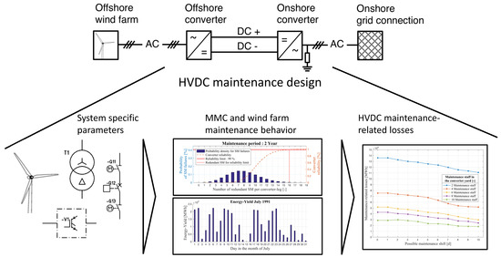
In order to improve the planning process, this study gives a detailed technical explanation of an HVDC energy export system for an offshore wind farm. In this, the different technical design aspects of the HVDC offshore and onshore stations are discussed. We quantify the MMC reliability under different maintenance strategies, and present the relationship between the maintenance period and MMC redundancy.
Based on a literature review, we show the various maintenance tasks for the HVAC and the HVDC components for the HVDC energy export system. Until today, there is no maintenance description for MMCs published. Therefore, the possible maintenance tasks for MMCs are discussed.
To analyze the influence of different design parameters and maintenance strategies on the maintenance-related losses of an HVDC energy export system, a maintenance model was built. The model is based on the previously described maintenance tasks and technical design aspects. In order to perform simulations, an energy time series is needed. Since no long-term energy data from offshore wind farms is available, a fictitious offshore wind farm and the Modern-Era Retrospective analysis for Research and Application (MERRA) dataset were both used to generate the required data [
15].
In order to demonstrate the model application, a case study was performed, in which different parameters, such as maintenance period, the number of maintenance staff, and the possibility to shift the maintenance starting time, were varied. Results of different simulation runs are shown and discussed.
The paper is organized as follows: in
Section 2, we described a reference HVDC energy export system. The different maintenance tasks for the HVDC energy export system are described in
Section 3. The developed model is presented in
Section 4. Following in
Section 5, the offshore wind farm used in the case study is described. In
Section 6, the case study is discussed, and finally, in
Section 7, a conclusion of the findings and an outlook for further research are given.
2. Reference HVDC Energy Export System
The HVDC energy export system in this study is designed for a transmission capacity of 1 GW, which is supposed to be a typical size for an offshore wind farm in the near future [
2].
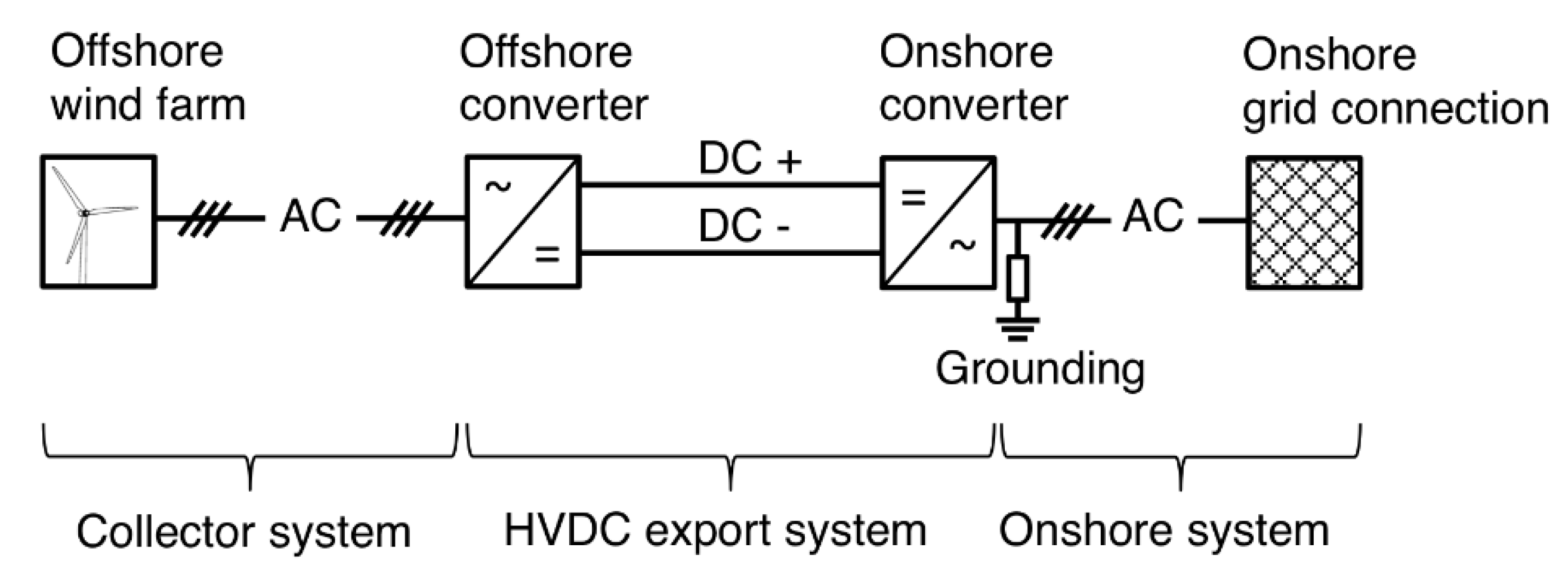
Figure 1 shows the typical schematic configuration of an offshore wind farm connected to the grid by means of an HVDC energy export system [
5].
The collector system includes the offshore wind farm and the inter-array grid for the wind farm. The HVDC energy export system includes the offshore and the onshore converter, as well as the DC transmission cables. The onshore system only consists of the grounding for the HVDC energy export system and the onshore grid connection point. The offshore and the onshore converters are the main parts of the HVDC energy export system.
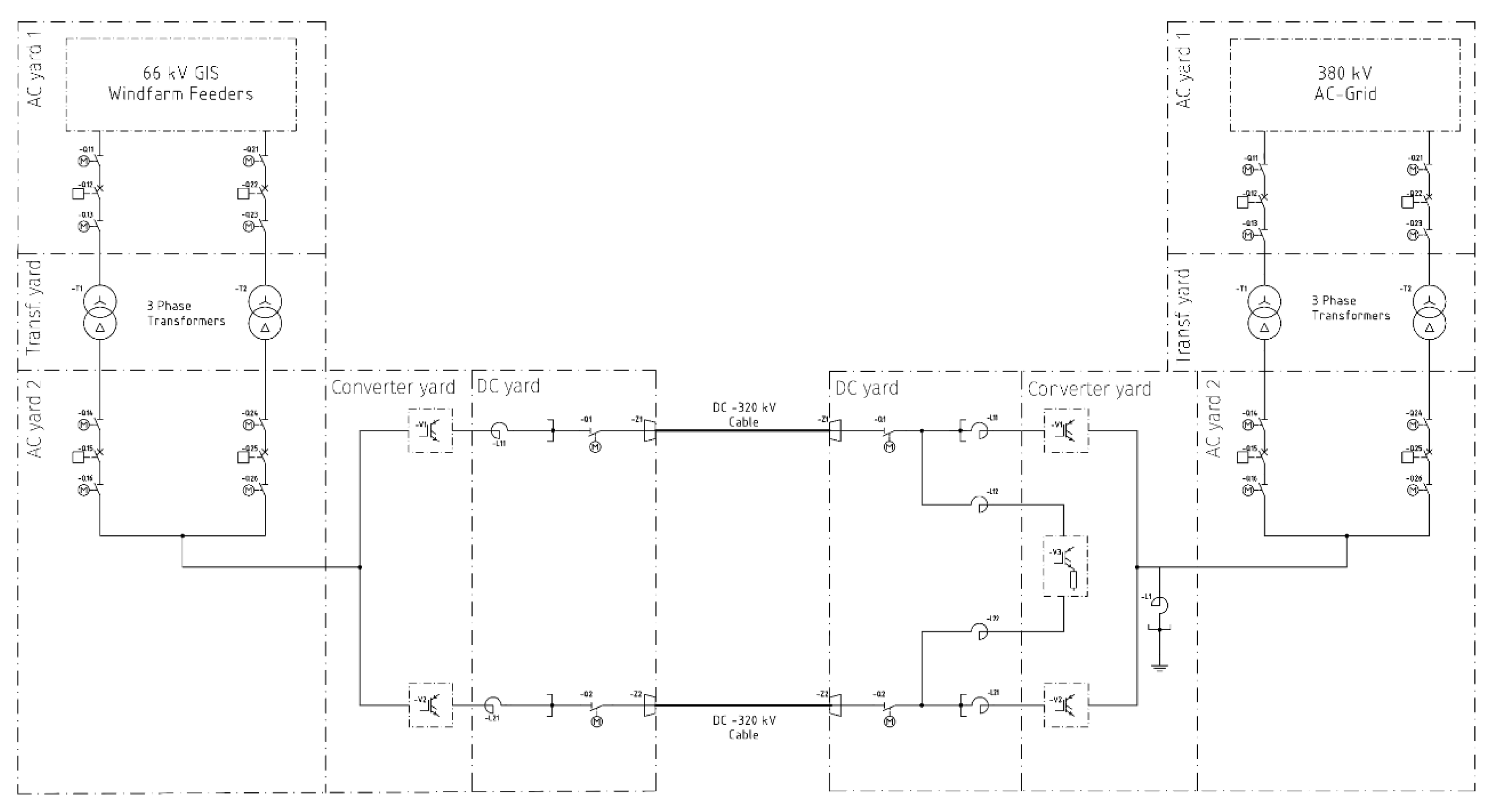
Figure 2 shows the detailed single line diagram (SLD) of the HVDC energy export system [
16].
In
Figure 2, the part to the left of the direct current (DC) cable represents the offshore station, and the part to the right represents the onshore station. On the offshore station, the AC yard 1 includes a 66 kV gas-isolated switchgear (GIS) (16 import feeders and two export feeders), that connects the wind farm to the two transformers. The two transformers (T1, T2) are located in the transformer yard, they transform the inter-array wind farm voltage from 66 kV to the transmission voltage of 320 kV. In the AC yard 2, a 320 kV GIS (Q14–Q26) connects the two transformers with the converter. In the converter yard, the MMC (V1, V2) converts the voltage from AC to DC. The DC yard includes the converter-reactors (L11, L21) and the direct current compact switchgear (DCCS) (Q1, Z1, Q2, Z2), which connects the converter to the DC cables.
Two DC subsea cables connect the offshore station and the onshore station. Today’s DC subsea cables require nearly no scheduled maintenance in their planned operating time [
17,
18,
19]. Therefore, the maintenance of the DC subsea cables is not further discussed in the following.
The structure of the onshore station is almost the same as the offshore station. The major difference between the two stations is that in the onshore converter yard, a chopper (V3) is installed. Using a chopper when connecting offshore wind farms with an HVDC energy export system is the most common method to avoid transferring onshore AC faults to the offshore wind farm grid [
20,
21,
22]. Due to the limited available space on the offshore station, the chopper is always installed in the onshore station [
16]. The advantage of using a chopper is that the wind farm can continue operating without any interruption in case a fault occurred in the onshore grid [
22,
23]. Today’s AC grids usually have a high quality of supply. For example, Tennet’s Annual Report states an AC grid availability of 99.9988%, and 17 number of interruptions for the year 2018 [
24]. By using the number of interruptions as an indicator to get a sense of how often the chopper is used, we can expect that the onshore grid is in normal operation most of the time; i.e., there is no failure, such as AC three-phase short circuits, in the grid. We therefore conclude that the DC chopper is only used for a small number of times a year, compared to the rest of the HVDC energy export system. On this basis, we assume that the wear and the maintenance work on the chopper are low compared to the MMC maintenance. Therefore, the chopper maintenance is not included in this study, and the following described maintenance tasks for the onshore and offshore stations are the same.
2.1. Converter (VSC Modular Multilevel Converter)
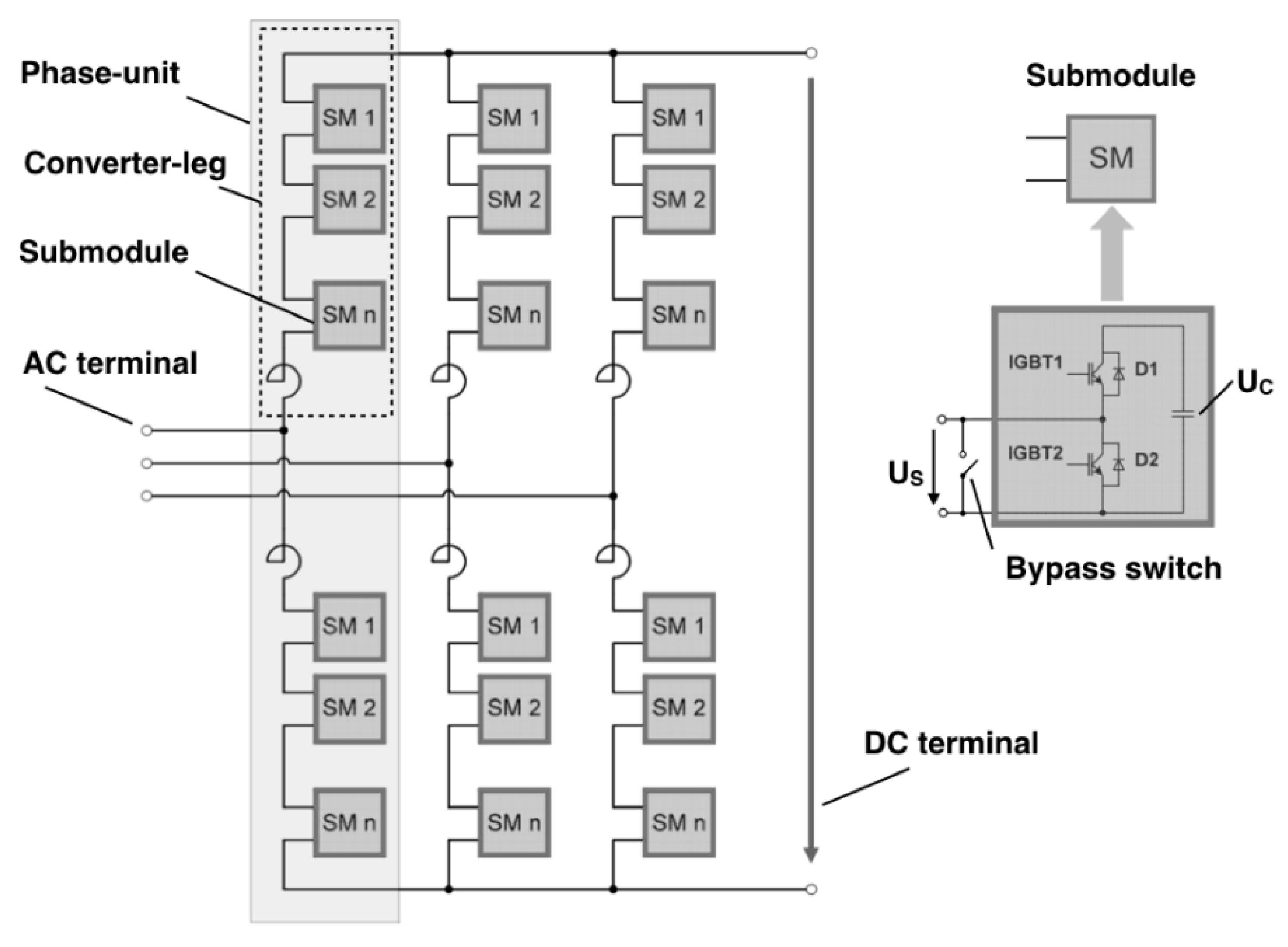
The MMC design consists of three phase-units between the positive and the negative DC terminal. Each phase-unit consists of a positive and a negative converter-leg. Each converter-leg consist of series-connected half bridge submodules (SMs) and a single series connected converter reactor. Each phase-unit is connected to one phase of the AC terminal.
Figure 3 shows the MMC structure and the detailed design of the half bridge SM [
7,
25].
The modular design of the MMC allows the individual adaptation of the converter to the technical requirements, e.g., transmission capacity, DC voltage and maintenance design [
7]. The maintenance design is mainly influenced by the number of redundant SMs. To ensure the functionality of the converter over a long period of time (maintenance period), redundant SMs are placed into each converter-leg. Two different operation schemes for SM redundancy are common: passive and active SM redundancy. In the passive operation scheme, the redundant SMs are on standby mode until a failure occurs in a normal SM. Then the faulty SM is bypassed through a bypass switch, and one of the redundant SMs becomes active.
In the active operation scheme, all SMs (redundant SMs and normal SMs) are actively operating in parallel. If a failure occurs, the failed SM will be bypassed automatically [
26].
In this study, the active SM redundancy is the scheme used today. It is assumed that the active SM redundancy is the today used scheme, because the control mechanism is simpler, and therefore, it is the more reliable method compared to the passive SM redundancy scheme [
27].
In order to calculate the number of redundant SMs, the minimum number of SMs
is required. The minimum number of SMs in one converter-leg results from the SM operation voltage
, the DC voltage
and the AC peak voltage
as described in [
28]:
The total number of SMs in the converter
results from the sum of the minimum number and the redundant number of SMs
in six converter-legs:
The redundant number of SMs depends on the maintenance period and on the reliability target for the converter. The relationship will be described in detail in
Section 2.2.
Table 1 shows the technical parameters of the energy export system, as seen in literature (cf. [
29,
30,
31]).
2.2. Converter Reliability
The converter reliability calculation in this study follows the general equation used in the literature (cf. [
32]). The equation describes the relative proportion of functioning components to be expected after a given time. Derived from this, the reliability function for one submodule,
, is given by (3).
where
represents the time in hours and
represents the SM hazard rate.
The hazard rate is considered constant over the whole lifetime, thus assuming constant random failures over the lifetime of the converter (cf. [
19]). The hazard rate of electrical components is often specified by the failures in time (FIT) value. FIT is the number of failures in one billion hours of operation:
The reliability of the converter can be described with the binomial distribution and
out of
majority redundancy. The
out of
majority redundancy describes the reliability of a system that consists of
components, and that is working only if at least
components in the system are able to operate. The general reliability function of the system is given by (5).
where
represents the number of all components in the system,
represents the number of components that is at least needed for operating the system,
represents the reliability function of one component, and
represents the time.
The resulting reliability function for one converter leg is given by (6).
Here, represents the total number of all SMs in one leg , and represents the redundant SMs per leg .
The MMC can only operate if the positive and the negative legs are able to operate. That is represented by a serial configuration, and results in the reliability function for one converter phase, as given in (7).
Due to the fact that the converter consists of three phases and operates only when all phases are working, the converter reliability,
, corresponds to the third power of the reliability of one converter phase, as given by (8).
With the parameters from
Table 1, the reliability of the converter can be calculated as a function of the number of redundant SMs and the maintenance period.
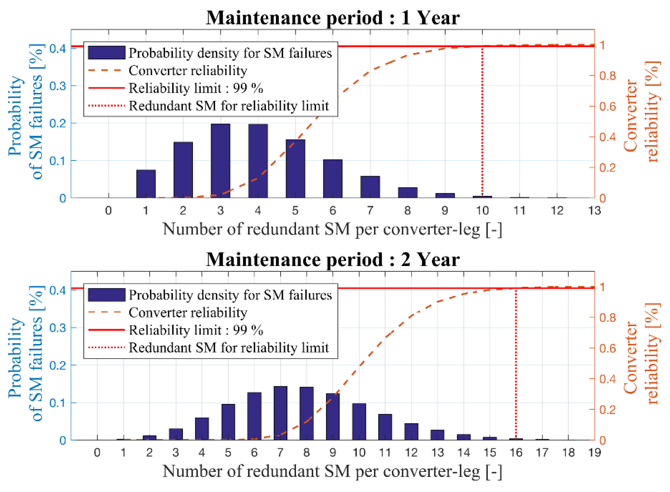
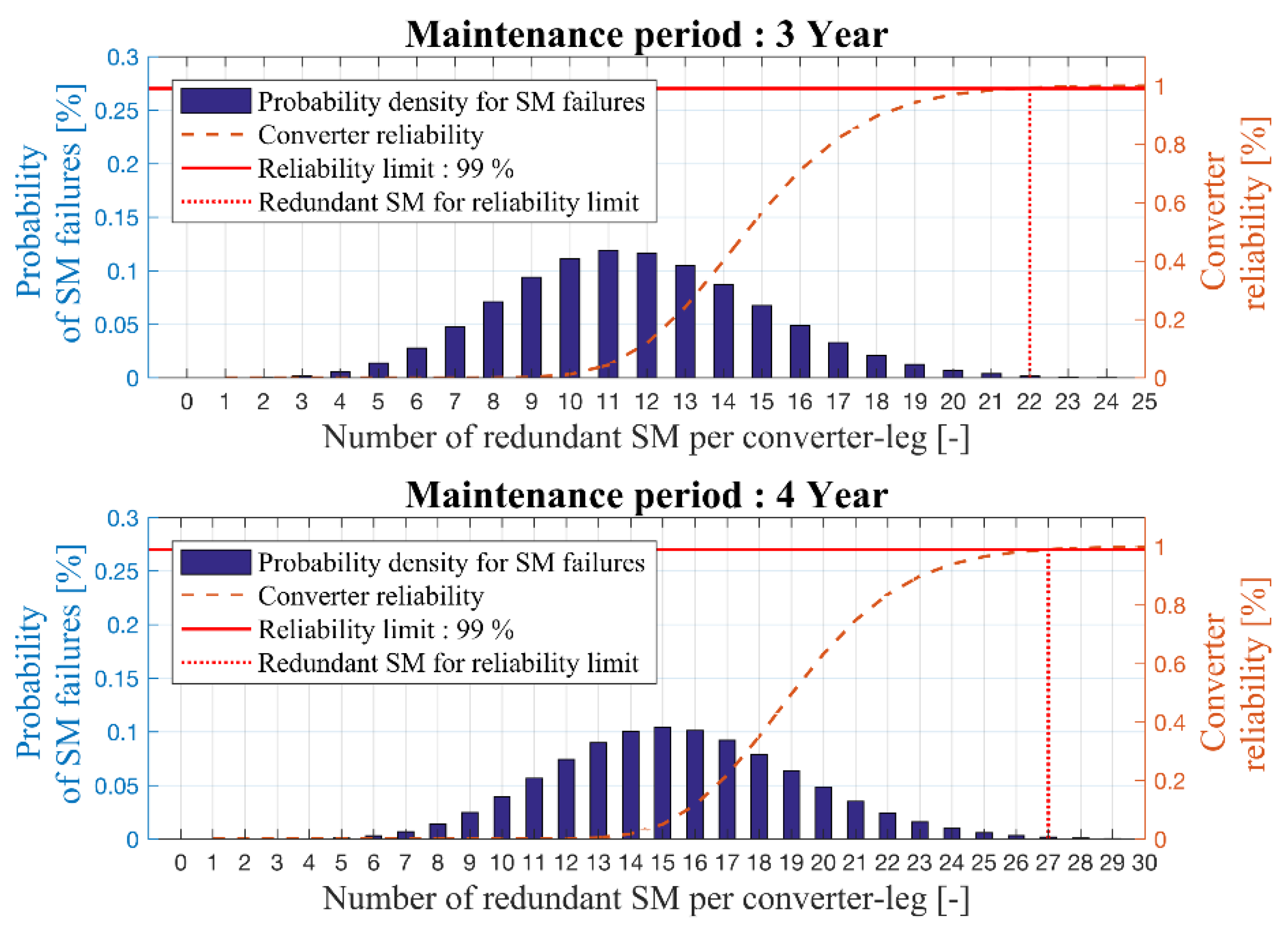
Figure 4 and
Figure 5 show this relationship for maintenance periods of one to four years with the resulting number of redundant SM per converter-leg at a reliability target of 99%.
The right ordinate shows the reliability function of the converter depending on the number of redundant SMs. The left ordinate shows the probability of SM failures per converter leg. In addition, a horizontal line represents the reliability barrier/target at 99%.
The dashed vertical line illustrates the resulting number of redundant SMs per converter leg that is needed to ensure the reliability target.
Table 2 summarizes the findings from
Figure 4 and
Figure 5. It displays the minimum required numbers of SMs for the operation, the required redundant SMs, and the sum of two, for the different maintenance periods. It can be concluded that the number of SMs for longer maintenance periods does not rise linearly. For a maintenance period of one year, 60 redundant SMs are needed. For two years, 96 SMs are needed. That results in an increase of 2.42% in the overall number of SMs. For an extension of the maintenance period to three years, 132 redundant SMs are needed (an increase of 2.36% in comparison to two years’ maintenance). For the four years’ maintenance period, 162 SMs are needed (an increase of 1.92% in comparison to three years’ maintenance).
It turns out that four-year maintenance periods do not require four times more redundancy than do one-year maintenance periods. This means that there must be an optimum number of redundant SMs, when comparing the total costs (capital costs) associated with additional SMs with the total maintenance costs (operational costs).
3. Maintenance
In order to ensure the reliable operation of electrical components, they must be maintained in specified periods [
32,
33,
34]. In this work, the transmission system is divided into different maintenance areas.
Figure 2 indicates the different electrical components, and the different maintenance areas of the stations marked with a dash-dotted lines. If one of the components has to be maintained, the component must be taken out of service. This implies that during this time, no energy can be transferred.
In relation to the HVDC energy transmission system, this means that if one component needs to be maintained, and there is no redundant component (cp. transformer yard), the whole transmission system has to be taken out of service for the maintenance time.
Table 3 gives an overview of the available transmission capacity in case of a maintenance in the different maintenance areas.
In order to analyze the influence of the individual maintenance tasks on the overall system, all relevant maintenance tasks were evaluated.
Table 4 shows an overview of all maintenance tasks, intervals, duration, and the assumed number of maintenance staff for the different maintenance works in the different maintenance areas.
3.1. MMC Maintenance
For maintenance work on MMCs, there are no reliable sources available. For this reason, assumptions must be made in this study for maintenance work in the converter yard.
The converter yard contains six converter legs, as shown in
Figure 3. During operation, the converter hall cannot be entered. Therefore, a certain preparation and follow-up time must be scheduled for the maintenance of the converter. The SMs are installed in towers, as described in [
16]. The primary maintenance task at the converter is assumed to be the replacement of defective SMs. The exchange of defective SMs is carried out by maintenance teams consisting of two persons. For the replacement of the SM, a working time of three hours is assumed for a maintenance team.
Table 5 shows the used maintenance parameters for the converter yard.
To calculate the maintenance duration for the converter yard, it is necessary to know the number of defective SMs at the maintenance time. This can be determined via the general probability function, used in the literature for electrical components (cf. [
32]), that a component (SM) has become faulty up to a certain time:
where the expected value of exchanged SMs
(i.e., defective) is calculated with
the maintenance period,
the total number of SMs in the converter, and
represents the SM hazard rate as FIT value given in
Table 1.
Table 6 shows the resulting numbers of defective SMs (rounded up) by performing the probability function (9), using values as defined in
Table 1 for the various maintenance periods.
It can be noticed that the relation between the expected number of defective SMs and the maintenance period is almost linear, although equation (9) contains a nonlinear part. After a two-year maintenance period, there are nearly two times more defective SMs than with one-year maintenance periods.
For calculating the maintenance time, the working time per day and the number of maintenance staff must be taken into account.
Table 4 shows the chosen maintenance staff for different maintenance areas.
For the calculation, a 12 h working time per day is assumed, and no shift work is scheduled. This means that within one day (24 h), up to 12 h of maintenance work can be performed.
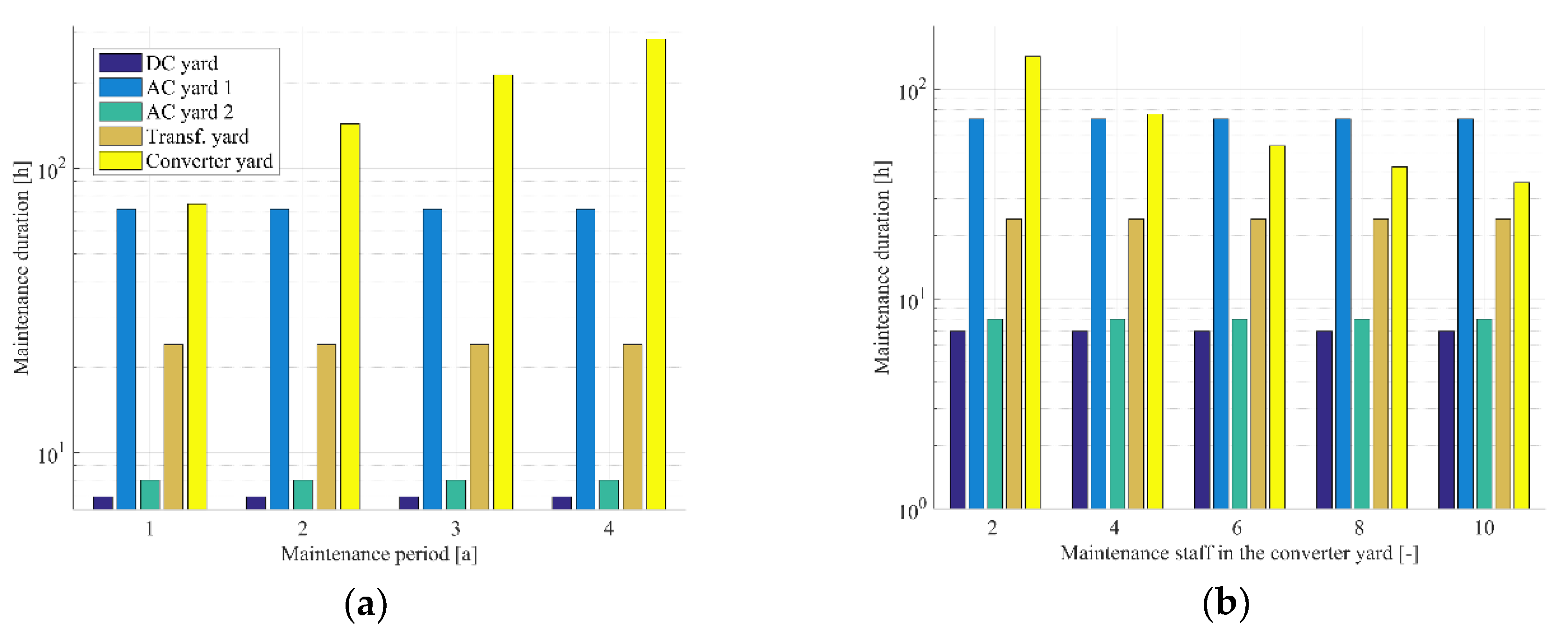
Figure 6 indicates the maintenance time for different maintenance areas over different maintenance periods, and different numbers of maintenance staff in the converter yard. In
Figure 6a, the x-axis represents the different maintenance periods for the HVDC energy export system, and the y-axis shows the maintenance time in a logarithmic scale. In
Figure 6b, the maintenance time is plotted over different numbers of maintenance staff in the converter yard at a maintenance period of two years. The x-axis represents the number of maintenance staff in the converter yard, and the y-axis shows the maintenance time in logarithmic scale.
In
Figure 6a, it can be seen that the maintenance time for the converter yard grows by 93% if the maintenance period is increased from one year to two years. The maintenance time for the converter yard is reduced by 53% if the number of maintenance staff is increased from two to four for a two-years maintenance period, as shown in
Figure 6b. It should be noted that the maintenance areas have different maintenance periods. For example, the AC yard only has to be maintained once every 25 years. This means that this area has less impact on maintenance-related losses in comparison to the transformer yard, which has a maintenance period of one year.
In conclusion, there should be an optimum for the number of maintenance staff in the different maintenance areas and the maintenance period, compared to the direct maintenance costs and the indirect maintenance costs.
3.2. Maintenance Date and Time Point
As shown in
Figure 6 and explained in
Section 3.1. (MMC Maintenance), the maintenance of an HVDC energy export system is associated with high personnel expenditure. Therefore, the maintenance date must be planned long-term in advance. For the planning of the maintenance date, it is essential to choose a time at which a low energy yield of the wind farm is expected. This date results from the distribution of wind speeds over the year.
At the wind measurement station FINO 1 in the north sea, the mean wind speed in June and July is 1.5 m/s below the mean annual wind speed of 10.0 m/s [
44]. From this it can be deduced that a lower feed-in power can be expected in summer than in winter. For this reason, maintenance of the HVDC energy export system always takes place in the summer months of June and July [
8].
3.3. Maintenance Assumtion and Model Simplifications
Some simplifications and assumptions are considered in this study, including station accessibility, individual maintenance costs and maintenance tasks on MMCs.
For offshore energy export systems, the accessibility of the two stations (onshore and offshore) is different, since the accessibility of the offshore station depends on weather conditions, such as wave height, visibility range, weather window and the availability of different ships or helicopters [
12]. In our study we focused on the dependency of MMC design aspects on the maintenance-related losses. Therefore, we excluded the exact analysis of the accessibility aspect.
It is important to precisely quantify the different cost positions (staff, material or transportation costs) when analyzing maintenance for offshore wind farms. Usually, it is very challenging to quantify the costs of individual positions; hence, it is difficult to investigate their influence on each other. For example, the exact value for staff salaries or transportation costs are not available in the literature [
12]. Therefore, we decided to focus on the missing energy yield. This represents only one specific maintenance cost factor, but it allows us to have a sense of how the missing energy export could behave regarding different design variations. To better understand the relation between the direct and indirect costs, a maintenance cost example was introduced in the end of
Section 6.
As mentioned in
Section 3.1. (MMC Maintenance), no reliable sources for maintenance tasks on MMC are available. For this reason, assumptions must be made for the maintenance tasks and durations.
Due to these assumptions and simplifications, the results of the study are considered optimistic in terms of the maintenance-related losses.
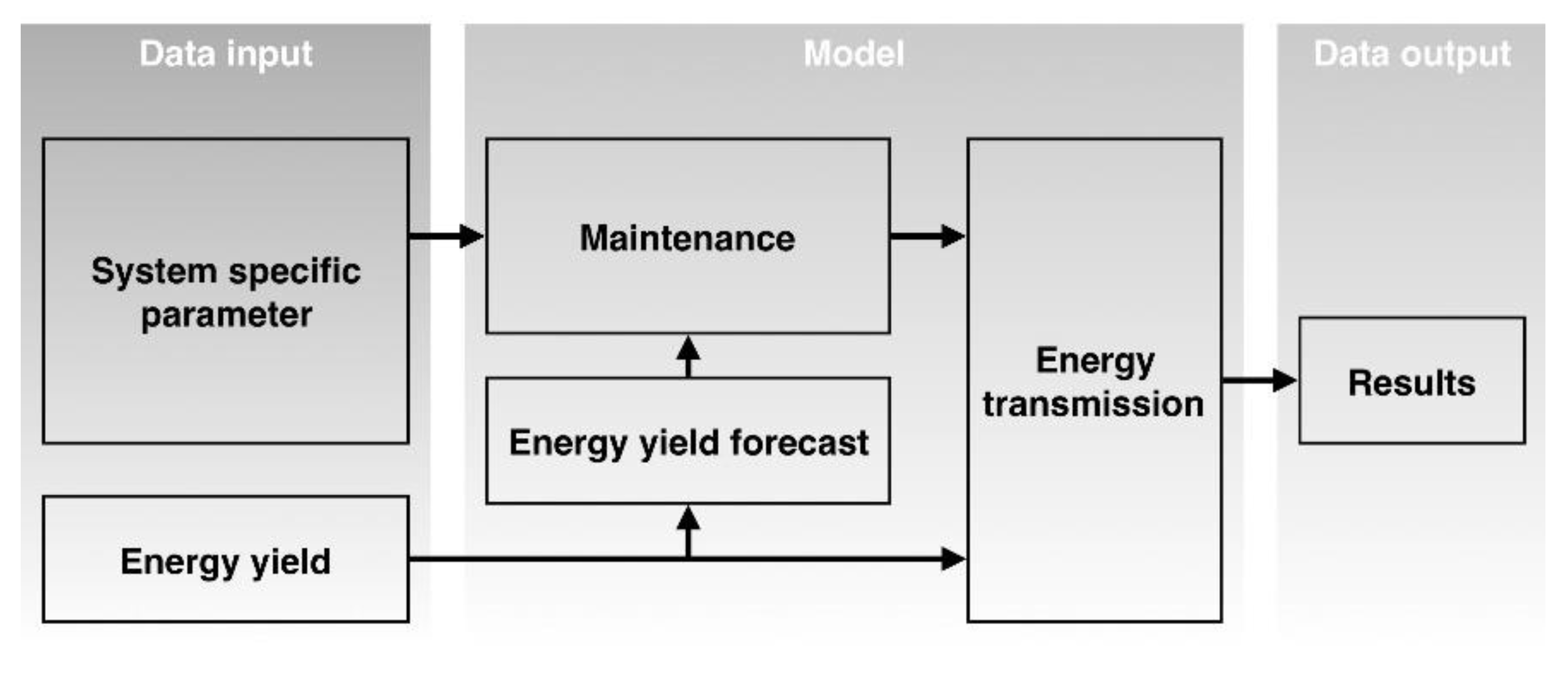
4. Model Description
The developed model, which can be seen in
Figure 7, is separated into three main sections: First the data input, second the model itself, and third the data output.
The data input is represented by the specific technical parameters for the HVDC energy export system (see
Table 1,
Table 2 and
Table 3) and a time series of energy yield data
for an offshore wind farm. The time series has a one-day resolution, where
represents a specific day in the total operating time. Instead of one representative year, we use yield data over the total expected operating time. For the case study described in
Section 6 for example, we apply past weather data from 1980 until 2010 to represent a 30 year long operating period of the energy export system.
The implemented model consists out of three sub models; the energy yield forecast model, the maintenance model, and the energy transmission model. The energy forecast model provides energy yield forecasts for different time horizons (up to ten days). It is assumed that a perfect energy yield forecast exists without any forecast error, which entails the highest savings potential for an optimized maintenance time.
The duration and periods of maintenance for the different maintenance areas are calculated within the maintenance model. All maintenance intervals of the different maintenance areas (see
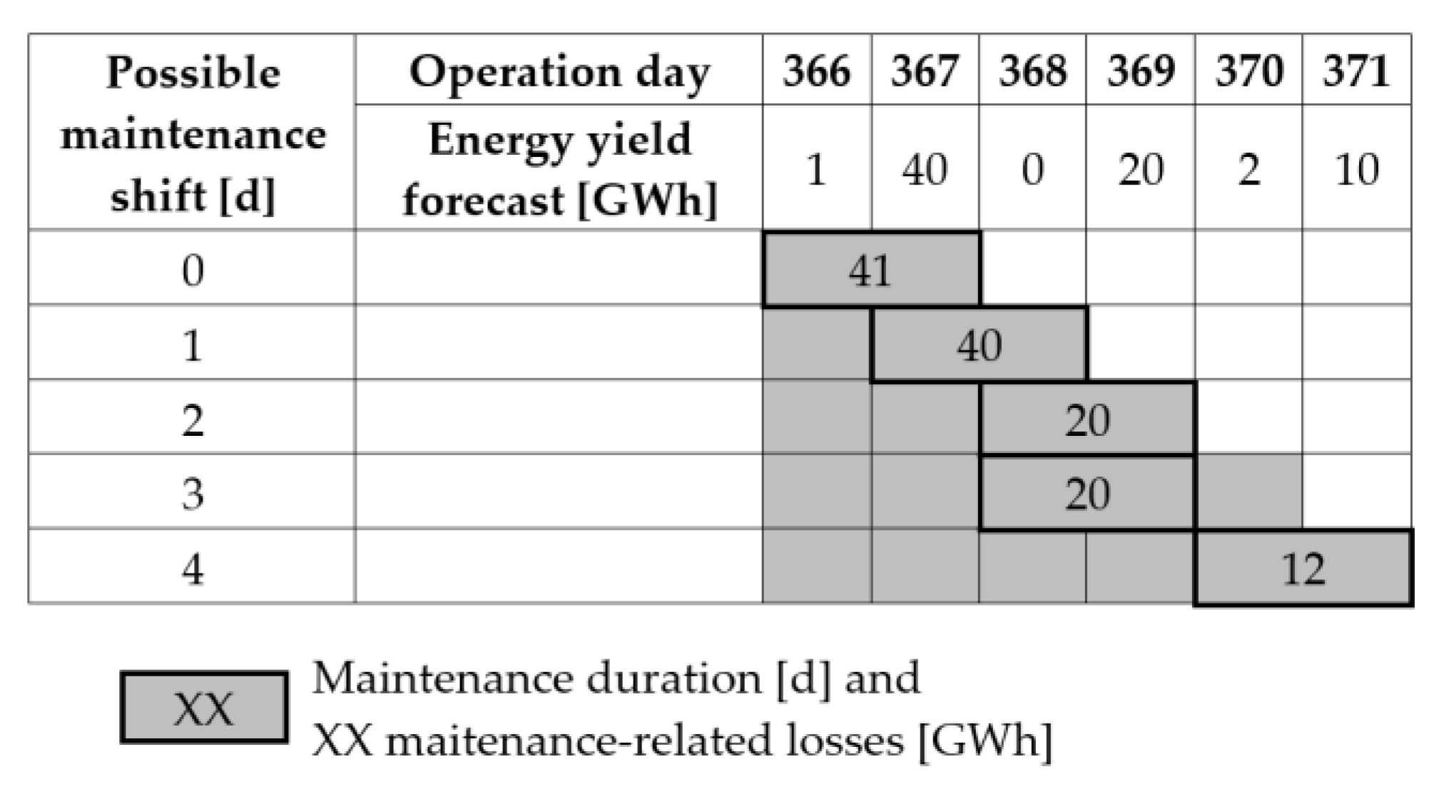
Table 4) are matched to the chosen maintenance period of the HVDC energy export system. Therefore, the maintenance model uses the system specific input parameters and the maintenance properties. In combination with the energy yield forecast, it optimizes the starting time of the maintenance in order to minimize the losses per maintenance.
Figure 8 shows one example of how the optimized maintenance is performed based on the energy yield forecast.
The maintenance model then creates a Boolean matrix , indicating whether any maintenance is required, or not, for each single day in the lifetime of the HVDC energy export system. This matrix is then imported by the energy transmission model.
The energy transmission model calculates, based on the original energy yield time series
, for every day, the losses that are caused by maintenance. The resulting maintenance-related losses for the life time of the HVDC energy export system
is given by (10).
The model developed here can map maintenance work up to a resolution of a quarter of a day. For analyzing and optimizing, the following three input parameters can be varied in order to reduce the maintenance-related losses: Maintenance period of the HVDC energy export system, number of maintenance staff and maintenance start day in combination with the energy yield forecast.
The model was implemented by using the software environment MATLAB 2016b from MathWorks [
45]. The code and data for the model is freely available online [
46].
5. Offshore Wind Farm
In the case study, a fictious offshore wind farm is assumed. The offshore wind farm, with a total capacity of 1 GW, consists of 125 wind turbines, and is located in the Eastern part of the North Sea. The center of the wind farm is at N 54° 56′ 22.4736 E 6° 56′ 44.3724 in the UTM (Universal Transverse Mercator) system.
The basis for the assumed wind conditions at the wind farm site are the Modern Era Retrospective-analysis for Research and Application (MERRA) data of the National Aeronautics and Space Administration (NASA). Various publications, such as [
47] and [
48], show that the MERRA data is a good basis for generating energy yield forecasts for offshore and onshore wind farm projects. In order to be able to capture the annual yield variations of the offshore wind farm, wind speed data from the period 1980 to 2016 is used as an operation period in this study. In the assumed operation period, the mean wind speed at the site is 8.5 m/s from April to September and from October to March is 11.3 m/s at a height of 103 m. The main wind direction at the wind farm site is West to Southwest.
The assumed wind turbine “W8000” has a rated power of 8 MW. The technical data of the system is listed in
Table 7. The wind turbines are set up in a cluster with a distance of 1000 m to the North and 1000 m to the East. By application of Pythagoras’ Theorem, this results in a distance of 1414.21 m between two wind turbines in the Southwest direction (main wind direction). That corresponds to nine times the rotor diameter, and is a common distance between offshore wind turbines in a park layout [
49].
The energy yield time series for the wind farm is created with the Wind Atlas Analysis and Application Program (WAsP) [
50]. Daily energy yield values were generated in the reference period from 1980 to 2016. The internal wake effects were considered with the FLaP wake model, and were taken into account when calculating energy yield [
51]. The wake effects of any of the surrounding wind farms were not considered.
The availability of a wind farm as described in [
52] depends on many factors, such as the maintenance concept or the location. It describes the period during which a wind turbine or an entire wind farm is ready for operation. Nowadays, the usual availability for offshore wind farms ranges between 75% and 95% [
52].
Based on the greater experience of operators, we expect the availability of offshore wind farms to further increase in the upcoming years. Therefore the assumed availability of the offshore wind farm in this study is 93%.
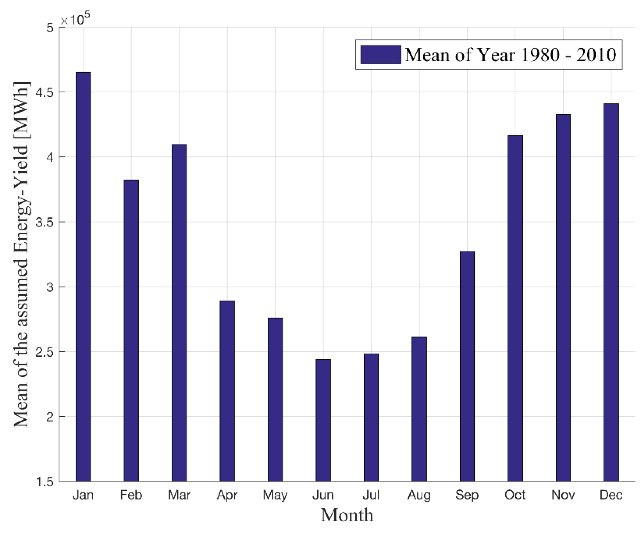
The potential gross energy yield of the wind farm calculated with the yield forecast described here, is transferred to the overall model described in
Section 4. Since wind farms are usually built and commissioned in the summer months, the operating period, and thus the yield period, is selected as 01.06.1980 to 31.05.2010.
Figure 9 indicates the mean energy yield produced by the wind farm under consideration of the availability of the wind farm in the period of 1980 to 2010.
6. Case Study Discussion
The model described in
Section 4 and the described wind farm in
Section 5 is used to analyze the possibilities of reducing the maintenance-related losses of an HVDC energy export system. The resulting energy yield forecast dataset described in
Section 5 is used as the energy yield input parameter. This dataset is used, because so far, no energy yield time series for an offshore wind farm over longer periods is available.
Three different parameter variations were tested to reduce the maintenance-related losses.
Table 8 gives an overview of the case study parameters and the parameters to be changed in the different variations.
6.1. Maintenance Period
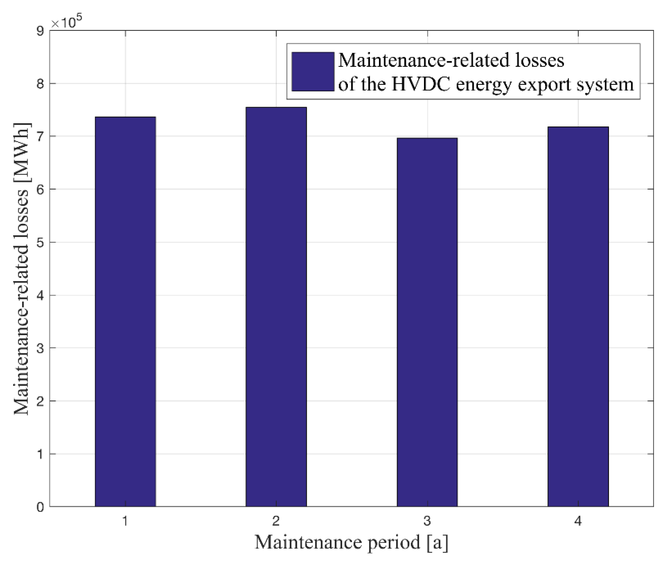
In the first scenario, the maintenance period of the HVDC energy export system is varied from the one year maintenance period up to the four year maintenance period. The number of maintenance staff members in the converter yard is set to two persons. The possible maintenance shift is set to 0 days. Therefore, the shift of the maintenance is not possible/allowed.
Figure 10 represents the results of the model calculation. It can be seen that the variation of the maintenance period from one year to four years influences the maintenance-related losses.
The x-axis shows the different maintenance periods, and the y-axis represents the maintenance-related losses. The blue bars show the maintenance-related losses over the total operation time. The result does not show a clear reduction in maintenance-related losses by only increasing the maintenance period from one year up to four years. One reason for this is that an extension of the maintenance period does not lead to a significant reduction of the maintenance time (see
Figure 6a). Since maintenance always takes place in the same days of the year, it can also happen that maintenance takes place in days when the wind farm would otherwise have a high energy yield. Therefore, the maintenance-related losses can also be higher for the two year maintenance period case than for the one year maintenance period case.
6.2. Maintenace Staff
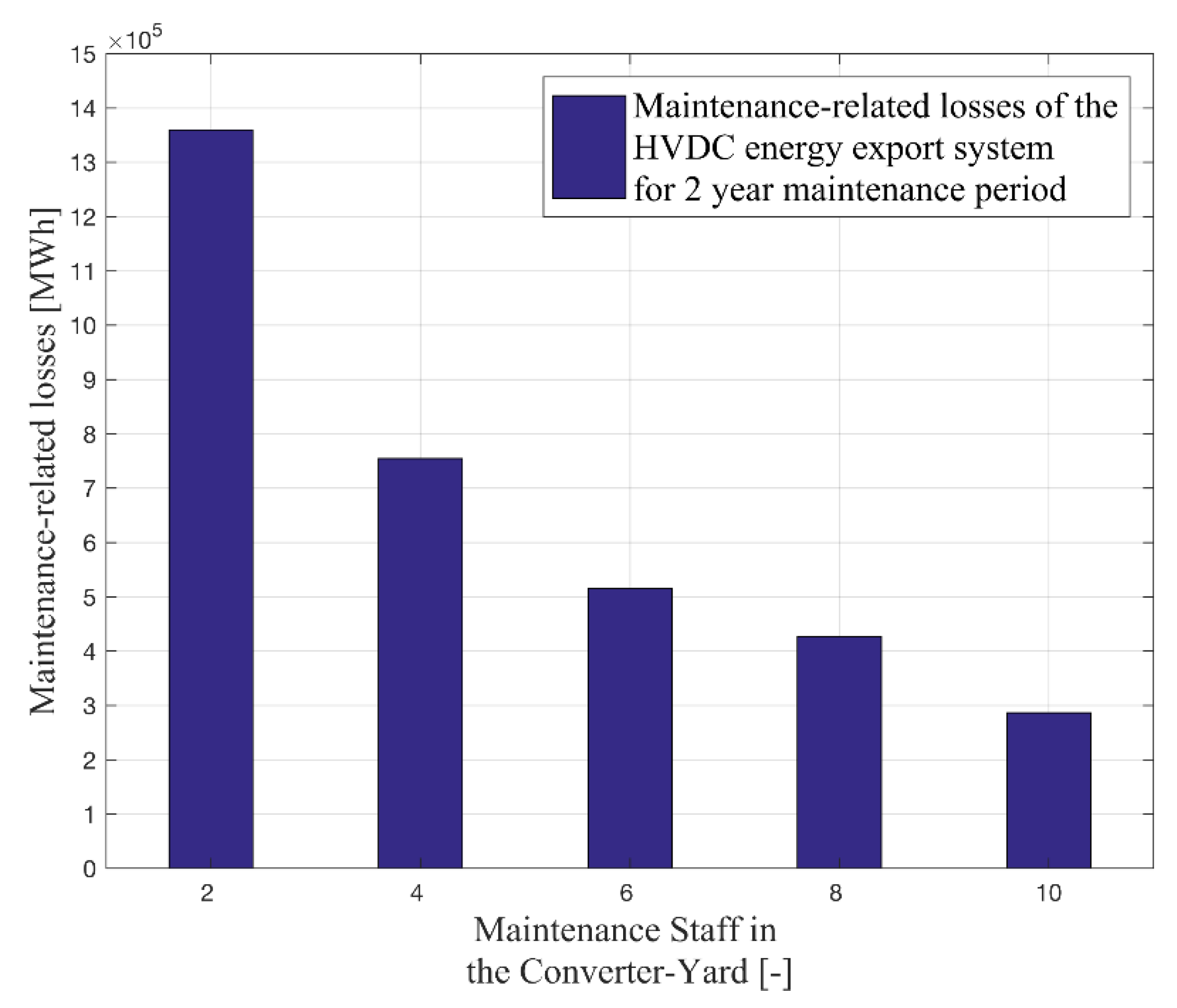
In the second scenario, the maintenance staff in the converter yard is varied from 2 to 10 persons. The maintenance period of the HVDC energy export system is set to a two-year maintenance period. Maintenance shift is set to 0 days. (i.e., no maintenance shift is not possible/allowed). The scenario with two staff members was considered the baseline case for all following calculations.
Figure 11 shows the result of the model calculation. It can be seen that the variation of the maintenance staff is reducing the maintenance-related losses.
The x-axis shows the different number of maintenance staff in the converter yard, and the y-axis represents the maintenance-related losses over the total operation time. It is noticeable that with the first doubling of the maintenance staff, maintenance-related losses can be reduced by 44.5 % (about 600 GWh maintenance-related losses were avoided). Further adding of maintenance staff only leads to a slight reduction 32% of losses (e.g., about 200 GWh could be saved by increasing staff from 4 to 6). The magnitude of the maintenance-related losses indicates that it might be profitable to carry out the maintenance with four or more people.
6.3. Maintenance Start Day
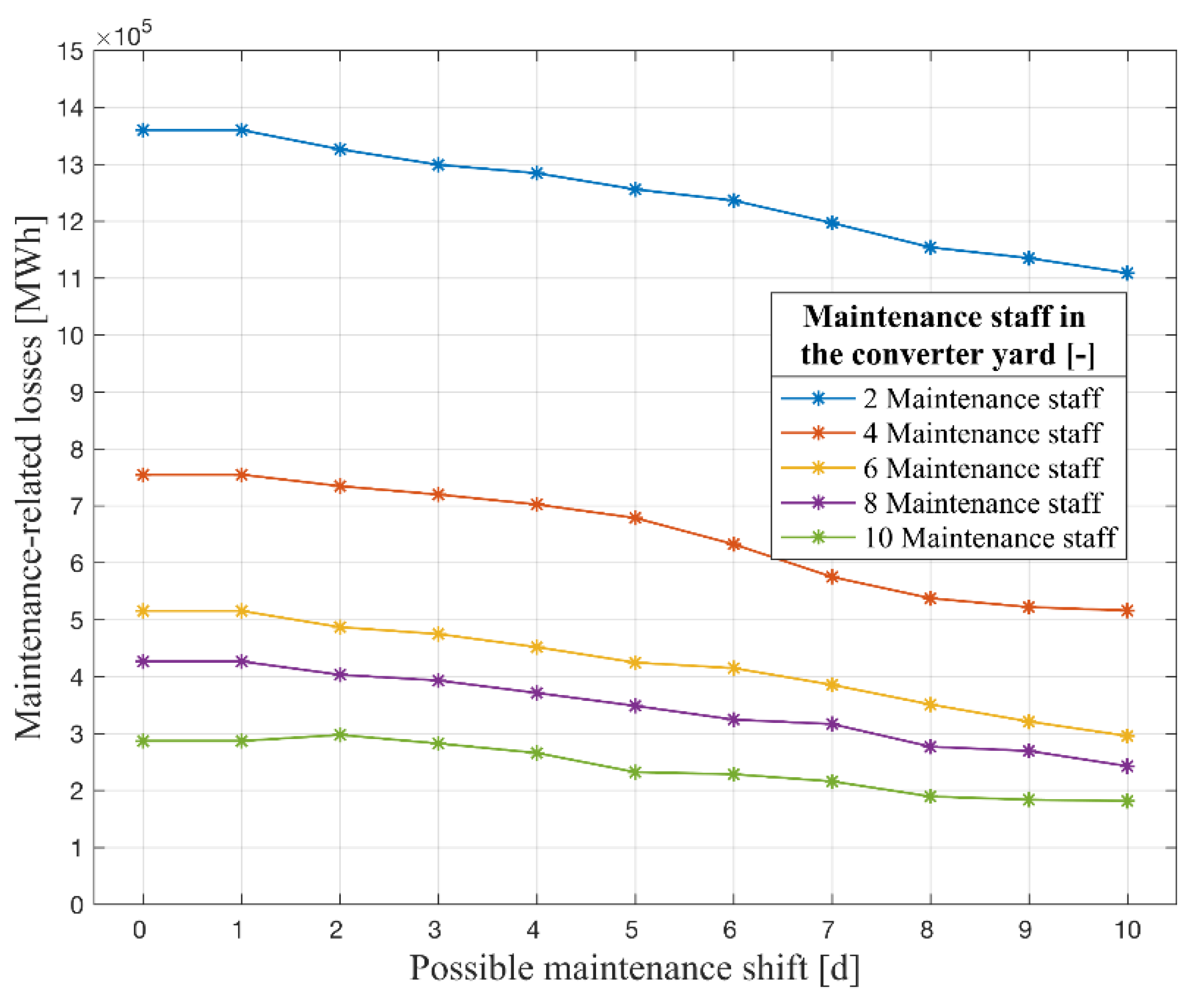
In the third scenario, the possibility to shift the maintenance start day is added. The model can now postpone the maintenance start day from 1 day up to 10 days to reduce the maintenance-related losses.
Figure 12 shows the results of the second and third scenario in relation to each other.
The x-axis shows different possibilities to shift the maintenance start day, and the y-axis represents the maintenance-related losses over the total operation time. The five differently colored lines represent the different numbers of maintenance staff in the converter yard.
It can be seen that the maintenance-related losses can be reduced significantly only if there is a shift margin of three days or more (up to around 50 GWh for the case of two maintenance technicians). It can also be seen that with the increasing margin to postpone the maintenance, the losses decrease. This can be explained by the fact that the model shifts the maintenance to a period in which the energy yield of the wind farm is low. The calculated maintenance-related losses should not be understood as an ultimate value, but it allows wind farm developers to get an idea of how the possibility to shift the maintenance could be profitable with respect to the losses.
The range of avoided losses indicates that it could be profitable to hire the maintenance staff for a longer period of time (multiple days). Within this period the choice of maintenance start day is optimized to minimize the maintenance-related losses.
With regard to the increase in maintenance staff, it can be seen that the curve flattens out with increasing maintenance staff. This means that postponing maintenance with increasing maintenance staff will have less effect upon maintenance-related losses.
6.4. Maintenance Costs Calculation
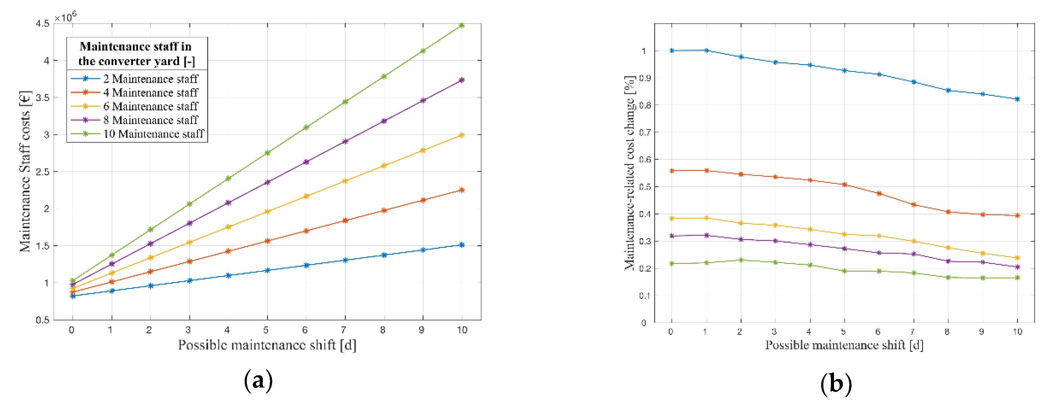
Based on the modeled maintenance-related losses, we calculated the maintenance-related cost change for the two parameters: the maintenance start day and the number of maintenance staff. The maintenance staff costs for the converter yard were calculated based on the modeled maintenance time for the converter yard and the maintenance staff cost parameter in
Table 8, which can be seen in
Figure 13a. The maintenance-related cost change was calculated by combining the direct maintenance costs (staff costs) and the indirect maintenance costs (lost remuneration), as seen in
Figure 13b.
In
Figure 13a,b the x-axis shows different possibilities to shift the maintenance start day. The y-axis in
Figure 13a represents the maintenance staff costs for the converter yard over the total operation time. In
Figure 13b the y-axis represents the maintenance-related cost change over the total operation time. The five differently-colored lines represents the different number of maintenance staff in the converter yard.
With the first doubling of the maintenance staff, the maintenance related cost can be reduced by around 44%. Additionally, it can be seen that the maintenance-related costs can be reduced by around 10%, only if there is a shift margin of six days (for the case of two maintenance technicians). It can be also seen that with an increasing margin to postpone the maintenance, the savings can be increased up to 19% (for the case of two maintenance technicians). This can be explained by the fact that the additional costs for maintenance staff are two orders of magnitude lower than the revenue losses. The range of maintenance-related cost change shows that it will be profitable to hire the maintenance staff for a longer period of time (multiple days). Within this period the choice of maintenance start day can be then optimized to minimize the maintenance-related losses, which further confirms what was concluded from
Figure 12.
7. Conclusions
In this paper, we applied a bottom-up approach to analyze the maintenance-related losses for an HVDC energy export system. A maintenance model was introduced for identifying the most significant factors affecting the maintenance-related losses.
In a case study, the model was used to analyze the potential to reduce maintenance-related losses for a 1 GW offshore wind farm. Three main factors were analyzed that influence the maintenance-related losses: duration of the maintenance period, the number of maintenance staff and the shift of the maintenance. In addition, we performed a maintenance cost example to better understand the relation between the direct and indirect maintenance costs of an HVDC energy export system.
It was found that changing the length of the maintenance period has less impact on the losses than the other two factors.
Regarding the number of maintenance staff, it is noticeable that with the first doubling of the maintenance staff with respect to the baseline case, maintenance-related losses and maintenance-related cost changes can be almost halved. Further adding of maintenance staff only leads to a slight reduction of losses.
With regard to the possibility to shift the maintenance date into times with a lower energy yield from the wind farm, it was shown that the maintenance-related losses can be reduced only if the shift margin is at least three days. With increasing the margin to postpone the maintenance up to 10 days, the maintenance-related cost change decreases down to 19%. By combining the increase of maintenance staff with the shift of maintenance time, it was shown that the curve of maintenance-related losses flattens out with increasing maintenance staff. This means that postponing maintenance with increasing maintenance staff will have less effect on maintenance-related losses and costs. It was also noticed that the staff costs for the converter yard had a small effect on the maintenance-related cost change compared to the maintenance-related losses, due to the difference in the order of magnitude between the direct and indirect costs of maintenance in the converter yard.
We have shown that optimizing the maintenance of an HVDC energy export system can decrease the maintenance-related losses for an offshore wind farm to almost one half with respect to the baseline case.
It was also shown that there is an optimum number of redundant SMs in relation to the maintenance period when comparing the total costs associated with additional SMs (increasing maintenance period) with the total maintenance costs.
In future work, industry data could lead to a more accurate model result. In addition, a detailed analysis of maintenance costs, such as traveling costs and costs for maintenance staff, could also be carried out.

 ,
, 


