Article

Wind Turbine Performance in Very Large Wind Farms: Betz Analysis Revisited

1
Department of Mechanical Engineering, Stanford University, Stanford, CA 94305, USA
2
Department of Aeronautics and Astronautics, Stanford University, Stanford, CA 94305, USA
*
Author to whom correspondence should be addressed.
Energies 2020, 13(5), 1078; https://doi.org/10.3390/en13051078
Submission received: 15 January 2020 / Revised: 21 February 2020 / Accepted: 25 February 2020 / Published: 1 March 2020
(This article belongs to the Special Issue State of the Art of Wind Farm Optimization)

Abstract

:
The theoretical limit for wind turbine performance, the so-called Betz limit, arises from an inviscid, irrotational analysis of the streamtube around an actuator disk. In a wind farm in the atmospheric boundary layer, the physics are considerably more complex, encompassing shear, turbulent transport, and wakes from other turbines. In this study, the mean flow streamtube around a wind turbine in a wind farm is investigated with large eddy simulations of a periodic array of actuator disks in half-channel flow at a range of turbine thrust coefficients. Momentum and mean kinetic energy budgets are presented, connecting the energy budget for an individual turbine to the wind farm performance as a whole. It is noted that boundary layer turbulence plays a key role in wake recovery and energy conversion when considering the entire wind farm. The wind farm power coefficient is maximized when the work done by Reynolds stress on the periphery of the streamtube is maximized, although some mean kinetic energy is also dissipated into turbulence. This results in an optimal value of thrust coefficient lower than the traditional Betz result. The simulation results are used to evaluate Nishino’s model of infinite wind farms, and design trade-offs described by it are presented.

1. Introduction

In a wind farm, each wind turbine will generally perform worse than an isolated turbine. The power loss with respect to an isolated turbine can be substantial, with typical losses of 10–20%, but as much as 40% in worst-case scenarios [1]. This degradation in performance occurs because the wakes of other turbines reduce the energy available in the wind. Despite the economic importance of these losses, a general, theoretical performance limit for wind farms is not known, as recently noted by Meneveau [2]. Wind turbine performance is often measured in terms of a power coefficient C P , which is the ratio of power generated by the turbine to the power available in the wind, if the turbine were not there. An inviscid and irrotational analysis of a streamtube encountering an idealized actuator disk illuminates a trade-off between turbine force and turbine power. This is the so-called Betz limit, which sets the maximum power coefficient to be 16 / 27 [3]. The aim of this study is to apply the same streamtube approach to numerical simulation data, which allows the relaxation of certain unrealistic assumptions in the classical analysis, namely that the turbine is isolated, the flow is irrotational, and the inflow is uniform.
Several studies have extended the Betz limit beyond its original assumptions. Garrett and Cummins [4] studied the effect of confinement, which is especially relevant to tidal turbines. Wagner et al. [5] suggested a correction to the calculation of power coefficient in order to account for the effect of shear. Both Chamorro and Arndt [6] and Draper et al. [7] derived a Betz limit for sheared, steady inflow. Their analyses assume an inviscid fluid, use the actuator disk approximation, and use streamtube arguments in the same spirit as the classical Betz analysis, but they differ in how the disk is modeled. Draper et al. use an actuator disk with uniform local resistance, whereas Charmorro and Arndt model the disk as applying a uniform force over its area, despite the variation in local velocity. None of the aforementioned studies consider the effects of turbulence or the wakes of other turbines. Luzzatto-Fegiz and Caulfield [8] have studied large eddy simulation (LES) and field data from finite extent wind farms using a boundary layer hypothesis to predict a fundamental limit to wind farm efficiency without appealing to streamtube arguments. Their analysis uses ideas from the study of canopy flows and does not resolve the flow around individual turbines. Other efforts to predict limits to wind farm efficiency, including in wind farms with finite size, have been made by Nishino [9,10].
The transport of momentum and energy have been previously studied in the context of wind farms and wind turbine wakes. Abkar and Porté-Agel [11] used LES to study mean and turbulent kinetic energy (TKE) budgets in an infinite wind farm in a conventionally neutral atmospheric boundary layer, although their work included Coriolis acceleration and focused on horizontally-averaged budgets. The dependence of mean kinetic energy budget on a turbine’s location in a wind farm has been examined by Cortina et al. [12]. The streamtube energy budget for a lightly loaded wind turbine in a small array was studied in a wind tunnel experiment by Lebron et al. [13]. They found that turbulence-related energy fluxes were of the same order of magnitude as power extracted by the wind turbine, and that production of TKE in the turbine wake was increased. Meyers and Meneveau [14] studied the geometry of streamtubes and some components of the momentum and energy budgets in an infinite wind farm setting. In the present work, this is extended by studying how all the budget terms are influenced by changing the turbine resistance.
The goal of this work is to use LES of an infinite wind farm to study the combined effects of shear, boundary layer turbulence, and the presence of other wind turbines on wind turbine performance. Using a suite of large eddy simulations (LES), turbine resistance is varied in an infinite wind farm with a well-studied “aligned” layout. Connections are drawn between the flow physics around individual wind turbines and wind farm performance trade-offs, which determine the optimal turbine thrust in the wind farm. This work is in the same vein as fundamental investigations of other variables affecting wind farm physics and performance, such as wind direction [15], turbine spacing [16], and atmospheric stability [11,17,18]. Especially as induction control strategies are being increasingly explored, understanding the flow physics of wind farms operating at different thrust coefficients becomes more important [19]. This study contributes to understanding of this issue in the limit of the infinite wind farm. All of the analysis in the present work is conducted through the lens of streamtubes, which are commonly used in the development of wake models to predict the velocity deficit behind a wind turbine. Extending this analysis to the flow in the wake shows how these two perspectives offer complementary views of the flow physics.
Section 2 derives expressions for the mean momentum and mean kinetic energy budgets for a mean streamtube around an actuator disk. Section 3 details the computational approach for the large eddy simulations and postprocessing used in this work. Section 4 reports the streamtube properties, as well as mean momentum and mean kinetic energy budgets. This includes breaking the momentum and energy budgets down into components and analyzing the changes in flow physics as turbine thrust is varied. Comparisons are also made between the wind farm LES and data from a simulation of an isolated actuator disk. Section 5 discusses the role of atmospheric boundary layer shear in modifying wind turbine performance, compares the simulation results to the wind farm theory of Nishino, and demonstrates design trade-offs that can be examined with Nishino’s model. Conclusions from the study are summarized in Section 6.

2. Momentum and Energy Budgets for a Streamtube

For LES of an incompressible, turbulent, inviscid ( R e ), steady-on-average flow, the transport equation for mean kinetic energy (MKE) can be written as Equation (1), using the Einstein summation convention.
x j ( 1 2 ρ u ¯ i u ¯ i u ¯ j ) = x j ( u ¯ j P ¯ + u ¯ i τ i j R + u ¯ i τ ¯ i j s g s ) S ¯ i j ( τ i j R + τ ¯ i j s g s ) + u ¯ j f ¯ j
Here, u i is the resolved fluid velocity vector, ρ is fluid density, and P is the hydrodynamic pressure. An overbar denotes time averaging, and a prime denotes fluctuations from the time-averaged quantity (e.g., u i = u i ¯ + u i ). The Reynolds stress tensor is given by τ i j R = ρ u i u j ¯ , the strain rate tensor by S i j = 1 2 ( u i x j + u j x i ) , and the subgrid scale stress tensor by τ i j s g s . The term f j represents a generic body force. Viscous effects on the resolved scales are neglected because the Reynolds number in wind farms is exceedingly high. The body forces of interest are due to turbines and to the body force driving the flow, which represents a steady pressure gradient in the streamwise direction due to geostrophic wind. Calaf et al. [20] discussed the appropriateness of neglecting resolved viscous forces, and of representing the effect of geostrophic wind with a body force. Integrating Equation (1) over some control volume (CV), employing the divergence theorem, and rearranging terms so that surface energy fluxes appear together on the left hand side, the following equation is obtained.
( 1 2 ρ u ¯ i u ¯ i u ¯ j + u ¯ j P ¯ u ¯ i τ i j R u ¯ i τ i j s g s ) n j d S = S ¯ i j ( τ i j R + τ ¯ i j s g s ) d V + u ¯ j f ¯ j d V
The dimension of each term in Equation (2) is Energy/Time, so each term expresses a rate at which the energy of the mean flow is entering or leaving the control volume via some particular physical process. The left hand side of Equation (2) represents exchanges of energy through the surface of the control volume. The four surface fluxes are advection of MKE by the mean flow, pressure work, energy transfer due to resolved turbulent stresses, and energy transfer due to subgrid scale stresses. The right hand side represents volumetric processes. These are due to production of turbulent kinetic energy (TKE), energy transfer into turbulence due to sub-grid scale stresses, and work done by body forces.
The control volume of choice in this study is a streamtube that is initialized as a circle concentric with the turbine disk. One such control volume is visualized in Figure 1. Because the streamtube follows the mean flow, the first two terms in the surface integral evaluate to zero on the tube surface, except for those surfaces at each end of the tube, which are defined to be perpendicular to the streamwise direction. For convenience, and because their contributions to the mean budget are small, all of the effects of the subgrid scale stresses are treated as another body force. With this choice, and substituting in for the relevant body force terms, the MKE budget becomes
( 1 2 ρ u ¯ i u ¯ i u ¯ j + u ¯ j P ¯ u ¯ i τ i j R ) n j d S = ( S ¯ i j τ i j R + u x ¯ f d P / d x ¯ + u x ¯ f t u r b i n e ¯ + u j ¯ f j s g s ¯ ) d V
where f d P / d x ¯ is the body force representing the streamwise pressure gradient, and f t u r b i n e ¯ is the streamwise body force due to the actuator disk. In the traditional analysis, the flow in the streamtube is treated as 1-D, considering only streamwise velocity and forces. Following this practice, velocity and pressure values are averaged over each streamtube slice, and a shape factor α is defined for MKE advection, also known as an energy coefficient or Coriolis coefficient [6].
α ( x ) = u ¯ x u ¯ i u ¯ i d A A u x ¯ 3
where A ( x ) denotes the area of the streamtube cross-section, and · denotes averaging over the streamtube cross-section. In addition, turbine power can be parametrized in terms of a power coefficient C P , which is computed in the following way, assuming the turbine is within the CV:
C P = u x ¯ f t u r b i n e ¯ d V 1 2 ρ A T U 3
where A T is the actuator disk area and U is the freestream velocity. The precise definition of U is discussed in Section 4.1. Other simplifications can also be made. Since f d P / d x ¯ is a constant body force, it can be factored out of the volume integral. Furthermore, the remaining integral u x ¯ d A d x = V ˙ , which is constant due to mass conservation in the streamtube. Arbitrary points x a and x b are defined as streamwise positions that mark the start and end points of the control volume. With these substitutions, Equation (3) becomes
ρ [ α 1 2 A u ¯ x 3 ] x a x b + [ A u ¯ P ¯ ] x a x b = ( u ¯ i τ i j R ) n j d S + ( S ¯ i j τ i j R + u j ¯ f j s g s ¯ ) d V      + f d P / d x ¯ V ˙ ( x b x a ) 1 2 ρ A T C P U 3
which can be rearranged into an alternate expression for C P .
C P = 1 2 ρ [ α A u ¯ x 3 ] x b x a 1 2 ρ A T U 3 i + [ A u ¯ P ¯ ] x b x a 1 2 ρ A T U 3 ii + f d P / d x ¯ V ˙ ( x b x a ) 1 2 ρ A T U 3 iii + ( u ¯ i τ i j R ) n j d S 1 2 ρ A T U 3 iv + ( S i j τ i j R ) d V 1 2 ρ A T U 3 v + ( u j ¯ f j s g s ¯ ) d V 1 2 ρ A T U 3 vi
The integral bounds are dropped to simplify notation. This equation is an alternative way to frame the energy budget for a control volume around a wind turbine. Since the objective of a wind turbine is to maximize the power produced, the advantage of this framing is that it highlights which physical processes contribute to power production. Term i is the change in MKE, term ii is the pressure work, term iii is the energy added volumetrically by the body force driving the flow, term iv is work done by Reynolds stresses on the surfaces of the control volume, term v is the production of TKE in the volume, and term vi is the work done by mean subgrid scale forces throughout the volume. Following a similar procedure with the streamwise momentum equation, analogous expressions for the thrust coefficient C T can also be written. This requires the definition of shape factor for streamwise momentum flux β , also known as a Boussinesq coefficient [6].
β ( x ) = x u ¯ x 2 d A A u x ¯ 2
The equations for thrust coefficient, analogous to Equations (5) and (7), are given below.
C T = f t u r b i n e ¯ d V 1 2 ρ A T U 2
C T = 1 2 ρ [ β A u ¯ x 2 ] x b x a 1 2 ρ A T U 2 i + [ A P ¯ ] x b x a 1 2 ρ A T U 2 ii + f d P / d x ¯ x a x b A ( x ) d x 1 2 ρ A T U 2 iii + ( τ 1 j R ) n j d S 1 2 ρ A T U 2 iv + ( f s g s ¯ ) d V 1 2 ρ A T U 2 v
Term i is the change in streamwise momentum, term ii is the pressure force, term iii is the “ d P / d x ” body force driving the flow, term iv is the normalized force due to Reynolds stress, and term v is the normalized force due to subgrid scale stresses.
The traditional streamtube analysis considers only the first two terms in Equations (7) and (10), with α = β = 1 . The third term would have appeared in the traditional analysis if the flow was driven by a body force. The following terms are the result of turbulence. The choice of control volume will affect the relative magnitudes of these terms, but since C T and C P are measures of turbine performance, the variations in the terms will always yield consistent C T and C P , provided the control volume encloses the entire actuator disk. In the limiting case that the control volume streamwise length goes to zero, only the pressure term remains, since it is discontinuous across the actuator disk. In the simulations, this is not achievable because the turbine force is smeared over the neighboring computational grid, so the grid must be considered when using Equations (7) and (10) to interpret the results. In Section 4, the relative magnitude of each term in the budgets is examined, as well as how these terms are affected by choice of control volume and local turbine thrust coefficient.

3. Simulation Method

For this study, several wall-modeled large eddy simulations of an “infinite” wind farm are conducted, largely following the method of Calaf et al. [20]. This is a half-channel flow with actuator disks, in which stratification, gravity, and Coriolis acceleration are neglected. The boundary conditions are periodic in streamwise and spanwise directions, with zero stress at the top boundary and a wall model applied at the bottom boundary. A constant body force is used to represent the effect of a streamwise pressure gradient.
The simulations are performed using a computational code, PadéOps-igrid, employing spectral differentiation in periodic directions and 6th order compact finite differencing otherwise. PadéOps is a code developed in the Flow Physics and Aeroacoustics Laboratory at Stanford University, which is freely available at [21]. The incompressible grid (igrid) branch is used in this work. This code has been validated on a number of incompressible flow problems, and has been previously used to study wind energy and atmospheric boundary layer flows [22,23,24]. The turbines are implemented as regularized actuator disks without rotation, using the same method as the JHU-LES code [20]. The Reynolds number is infinite, meaning there are no viscous forces on resolved scales. Full details regarding subgrid scale model, time stepping, and other aspects of the solver can be found in Appendix A of Ghate and Lele [22].
The infinite wind farm regime is only reached once the internal boundary of the wind farm within the atmospheric boundary layer (ABL) has grown to the full height of the ABL, meaning that as a simulation technique, it approximates the flow in wind farms which are much longer in the streamwise direction than the spanwise direction [25]. While the infinite wind farm method is less realistic than precursor methods [26], it has been widely used to study various aspects of wind farm physics, including scalar transport [27], the effect of wind turbine spacing [16], and atmospheric stability [28]. Also, periodic boundary conditions in the spanwise direction are still commonly used in simulations using an ABL precursor to study finite-extent wind farms.
A cartoon of the domain used in the wind farm simulations is shown in Figure 2. All cases use same disk diameter and “4 × 6” planform layout. They are differentiated only by C T , the local thrust coefficient, which is used to determine the thrust the actuator disk exerts instantaneously on the flow based on the velocity at the turbine.
F t u r b i n e ( t ) = C T 1 2 ρ A T 1 A T d i s k u x ( t , y , z ) d A 2
Unlike C T or C P , C T is an input specified to the simulations.
Applying the streamtube control volume analysis to simulation data requires careful attention to the numerical implementation of the actuator disk. In order for the budget Equations (7) and (10) to be satisfied, the streamtube must contain the entire actuator disk. In the classical analysis, this means that the streamtube diameter at the disk is equal to the turbine diameter. However, this streamtube is too small for simulation data, because the actuator disk force is smeared over the numerical grid for stability. To resolve this, the streamtube is initialized so that it captures 99% of the force exerted on the flow by the disk. For the wind farm cases presented here, this diameter is 1.349 times the actuator disk diameter. This means that the streamtube is oversized by 2.1 grid points in the y-direction, and 4.5 grid points in the z-direction.
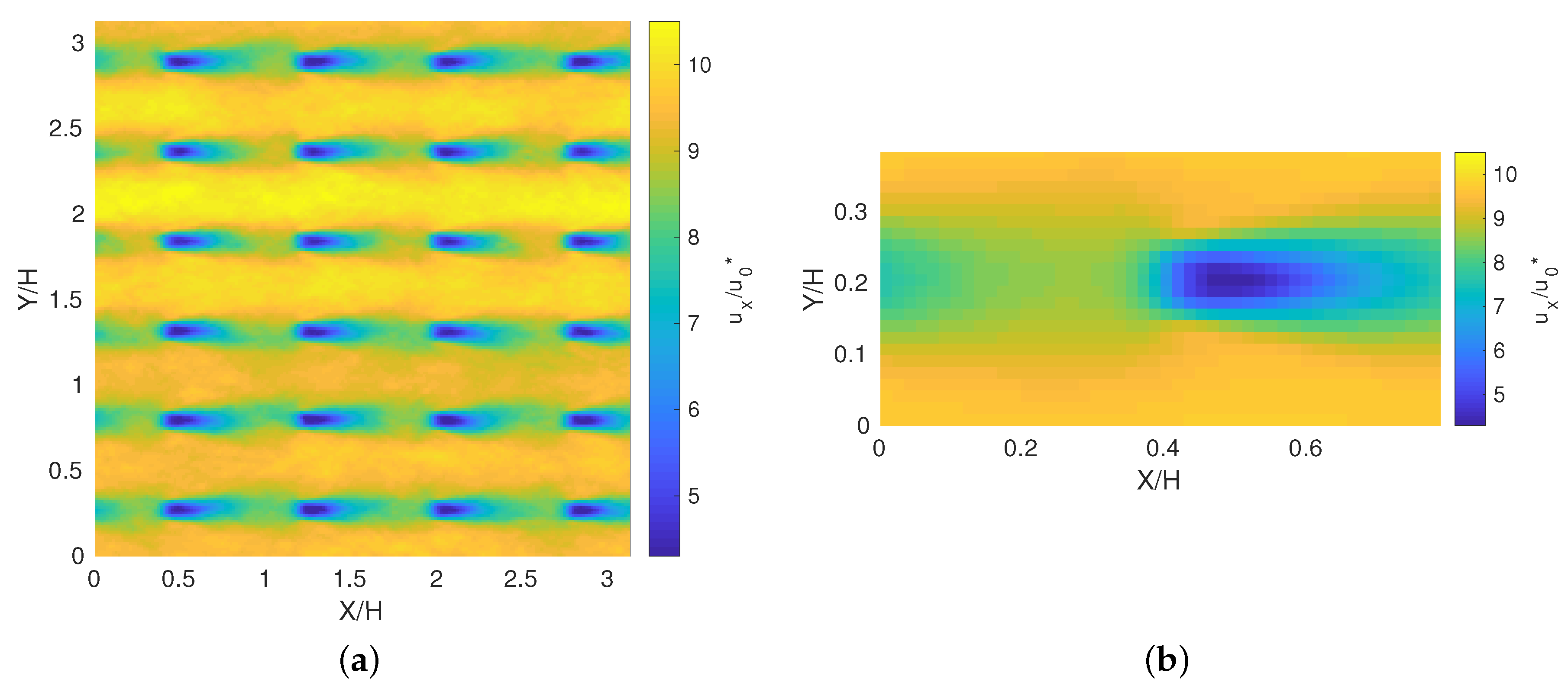
To compute the mean streamtubes, as well as all streamtube properties and budgets, the velocity field is averaged in time and over an ensemble of all turbines in the domain. For example, Figure 3 shows the time-averaged streamwise velocity at hub height for one wind farm simulation. In Figure 3a, some evidence of high-speed streaks between the turbine rows is visible. This has been observed in other wall-bounded flows, and wind farm LES in particular, where the streamwise domain is not large enough to allow flow structures to break up [29]. This effect is mitigated by ensemble averaging over the 24 turbines in that domain, as shown in Figure 3b.
The streamtubes are initialized with 100 points around the circumference of the actuator disk, and fluid particle trajectories for those points are computed downstream and upstream of the turbine based on the mean flow field described above. The trajectories are computed with RK4 time stepping, using linear interpolation of the mean velocity field to define the velocity between grid points. Once the trajectories are obtained, streamtube cross-sections at y z planes are defined by linearly interpolating the 100 trajectories at specified x locations. These streamtube cross-sections, defined by 100 points around their perimeter, are used to compute various area and volume integrals in Section 4. Area integrals, such mean velocity in the streamtube at a streamwise location, are computed by discretizing the streamtube cross-section area with 100 points in the radial direction, using the centroid of the boundary points as the origin. Then, the integral is evaluated in polar form using the midpoint rule, using spline interpolation to obtain the function values in the midpoint of the polar cells. Volume integrals in the streamtube are computed in a similar way, by taking area integrals at each station, and then integrating in the streamwise direction with fixed step size using the trapezoidal rule [30].
The streamtube control volume analysis could also be applied to finite wind farms, with two important changes. First, the ensemble averaging over all turbines would be omitted, or replaced by averaging within rows, if the wind farm is spanwise homogeneous. Second, the energy budgets for each row would need to be considered separately, and the number of rows would be a design variable in the optimization, along with C T .

4. Results

The wind farm cases analyzed in this section were chosen to study a wide range of thrust coefficients C T for a commonly studied layout, the 4 × 6 aligned grid. Nine different cases were simulated: C T = [ 0 ,   0.1 ,   0.3 ,   0.6 ,   1.33 ,   2.0 ,   3.0 ,   4.0 ,   6.0 ] . Table 1 lists the parameters common to all cases. Previous studies have focused on C T = 1.33 , which is regarded as a typical value, with fewer cases conducted at C T = 0.6 and C T = 2.0 . The theoretical Betz limit occurs at C T = 2.0 . The additional cases at higher and lower values of C T presented here help to resolve the C T   v s .   C P curve, aid with validating Nishino’s model, and are useful for understanding trade-offs among energy budget terms which modify the Betz limit in this setting. The cases with C T = [ 0.6 ,   1.33 ,   2.0 ] in this work correspond respectively to cases C, A, and B from Calaf et al. [20].
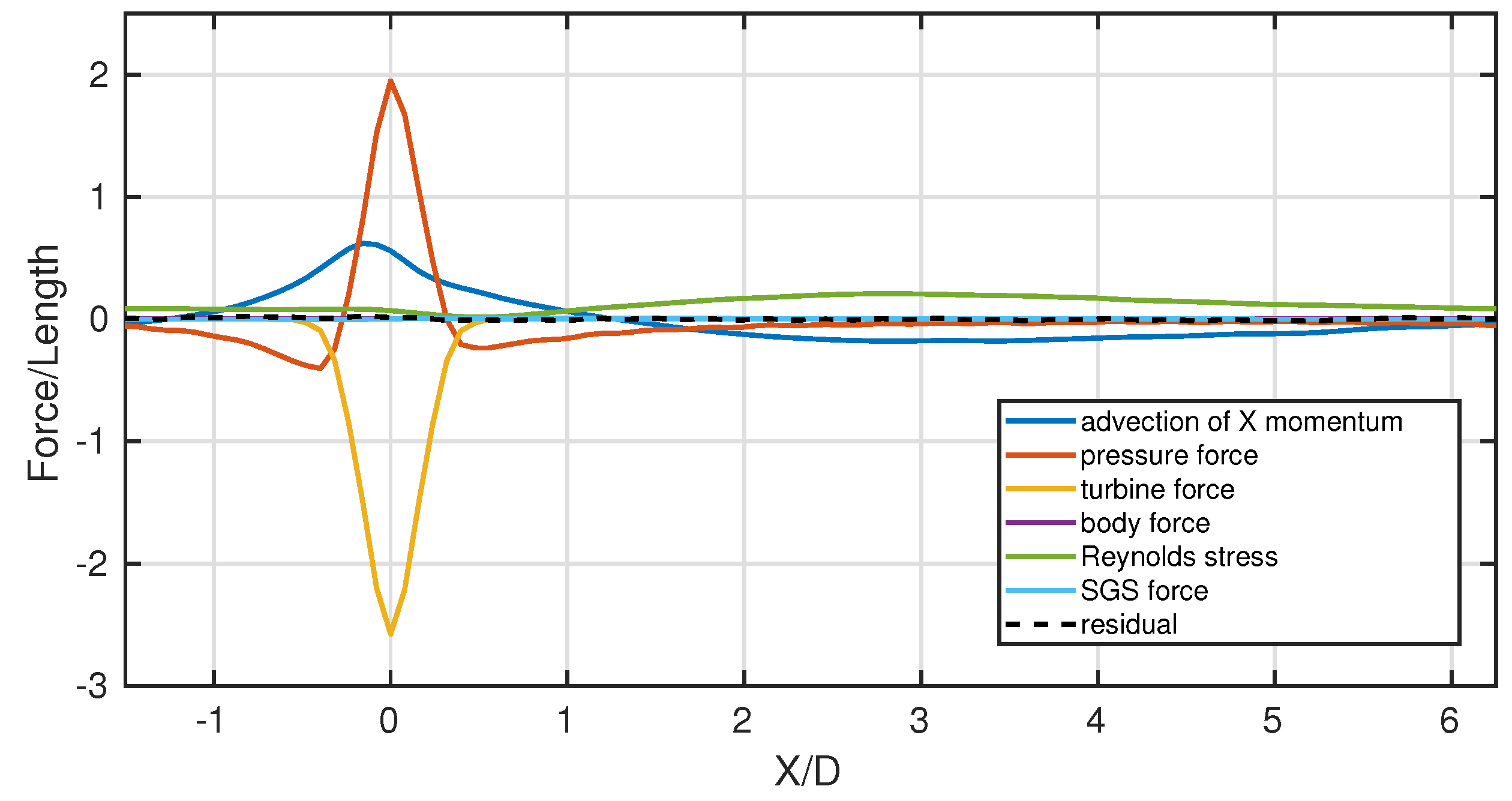
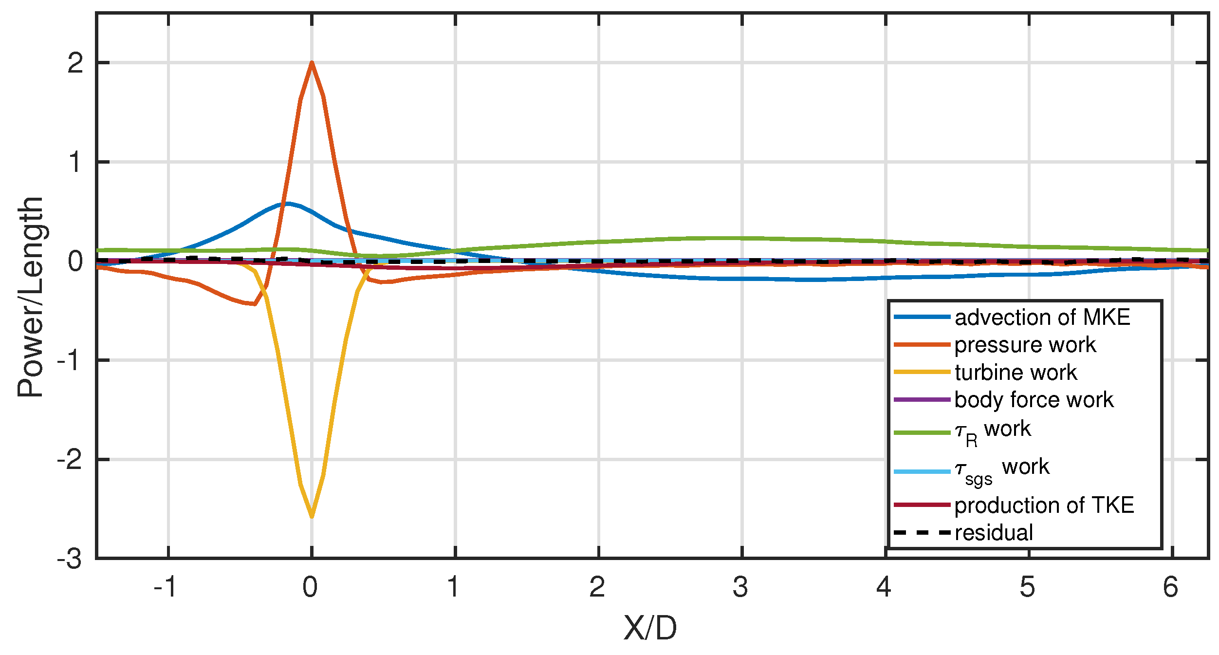
Using the streamtube control volume discussed in Section 2, Figure 4 shows each term in the Reynolds-averaged streamwise momentum equation integrated over the streamtube cross section. Each term is normalized such that the turbine force term integrates to unity. Figure 5 shows the same for each term in the MKE Equation (1), normalized by the integrated turbine power. Only the budget for C T = 1.33 is plotted in detail, but budgets were computed for all cases, and the influence of C T is presented in Section 4.2. Positive values in the budgets correspond to sources of mean momentum or mean energy, and negative values to sinks. The mean streamwise momentum and mean kinetic energy budgets provide very similar pictures of the physics for C T = 1.33 , indicating that the energy budget is dominated by terms related to mean streamwise momentum. For this reason, only the energy budget is discussed in detail.
A prominent feature in the mean kinetic energy budget is the turbine work, which is the primary energy sink in the streamtube control volume. In the immediate vicinity of the turbine, pressure work and MKE advection are the primary sources of energy. However, because the wind farm is periodic, and hence the mean pressure and velocity fields are periodic, the net MKE advection and pressure work terms are very small when integrated over the entire streamtube volume. Although the work done by Reynolds stresses is generally small at each location along the streamtube, it is always positive, and so globally, it supplies the energy that is extracted by the turbine. This is the same physical mechanism as the frequently described vertical flux of kinetic energy [20,25,26]. From the perspective of the streamtube control volume, there is a lateral ( u ¯ x u x u y ¯ ) as well as vertical ( u ¯ x u x u z ¯ ) kinetic energy flux. The lateral kinetic energy flux was also noted by Cortina et al. [17] in wind farms with large spacing between turbines. In the wake of the turbine, some energy is removed from the mean through the production of turbulent kinetic energy (TKE). Most of the TKE production occurs between 0 and 3 diameters downstream of the turbine. In agreement with Lebron et al. [13], both TKE production and energy flux due to Reynolds stresses peak in the wake of the turbine. After about 2.5 diameters downstream of the turbine, the Reynolds stress work and MKE advection terms roughly balance, indicating that the energy transported in by turbulent stresses is stored in mean kinetic energy.
It is also worth commenting on the relevance of the MKE budget to the total energy budget (MKE + TKE). In the streamtube control volumes, TKE is small compared to MKE for small values of C T . Around C T 0.6 , TKE becomes comparable to MKE, especially in the turbine wake, eventually becoming larger than MKE for C T > 2 . This is due to large velocity deficit and intense turbulence created by large C T . It does not imply that the TKE budget is of greater importance to wind turbine performance for those cases, because the fluctuations’ contributions to total turbine power are always small: less than 3% for C T 3 , and less than 6% for C T 4 .
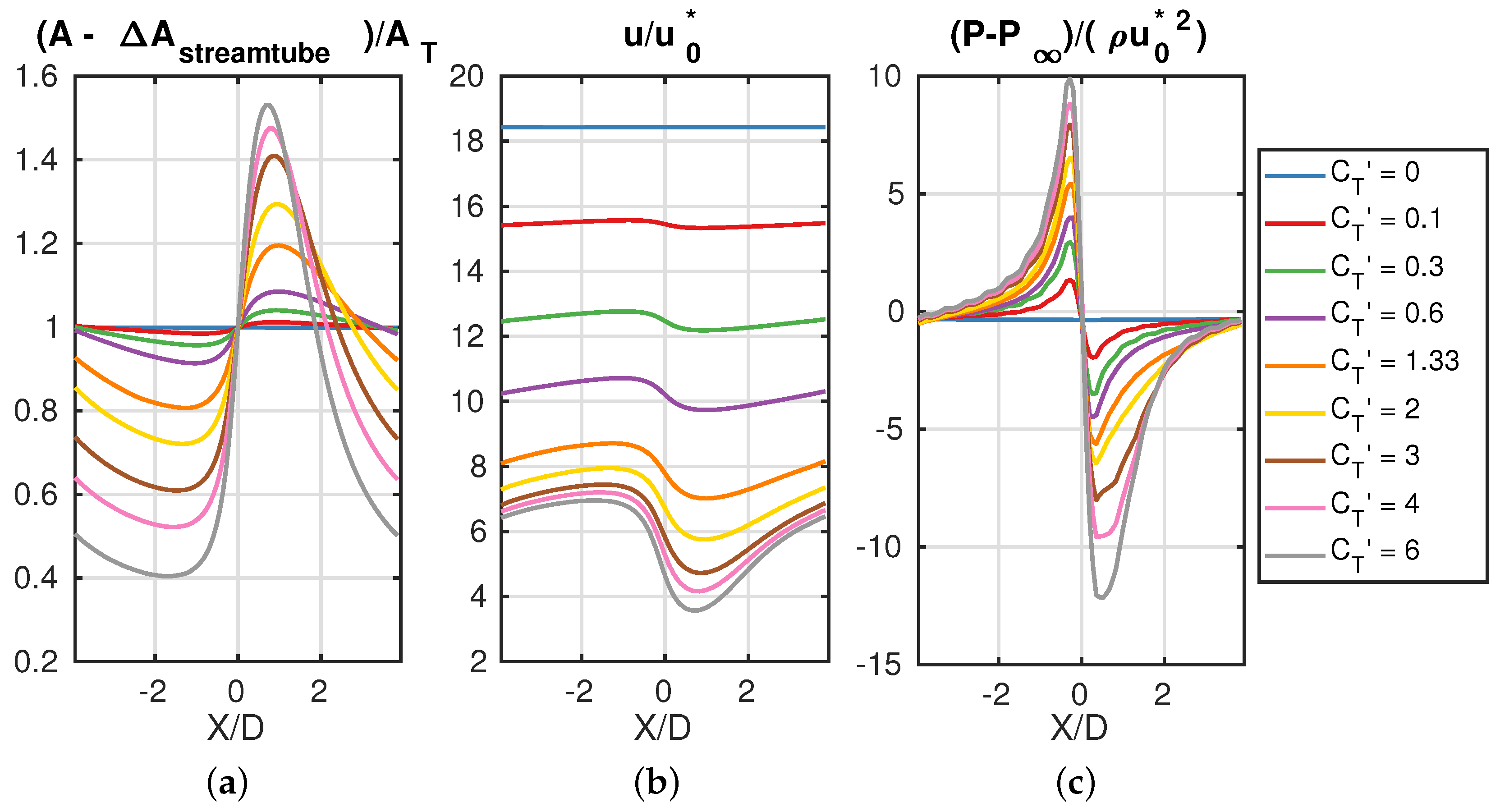
In order to interpret budgets as C T is varied, it is helpful to look at quantities averaged over streamtube cross-sections, such as streamtube area, velocity, and pressure. These are plotted in Figure 6. This allows comparison to the classical Betz analysis, which considers a one-dimensional velocity and pressure field inside the streamtube. As C T is increased the pressure difference across the disk grows, and the velocity drops more as well. Note that as the thrust coefficient is increased, the average velocity in the streamtube also decreases. This happens because the turbines extract momentum from the flow, slowing it down. Because the streamtube is mass-conserving, these observations about velocity have straightforward connections to the cross-sectional area of the streamtube. As the streamtube approaches the turbine, it expands, and as the wake of the turbine recovers, the streamtube contracts (also seen in Figure 1). This is in contrast to the classical streamtube analysis, where there would be an upstream and downstream state for both velocity and cross-sectional area. Because these results are for turbines situated in an infinite wind farm, the velocity and area are instead periodic in the streamwise direction. For low values of thrust coefficients, the area varies only slightly, maintaining a nearly cylindrical shape, as observed by Lebron et al. [13].
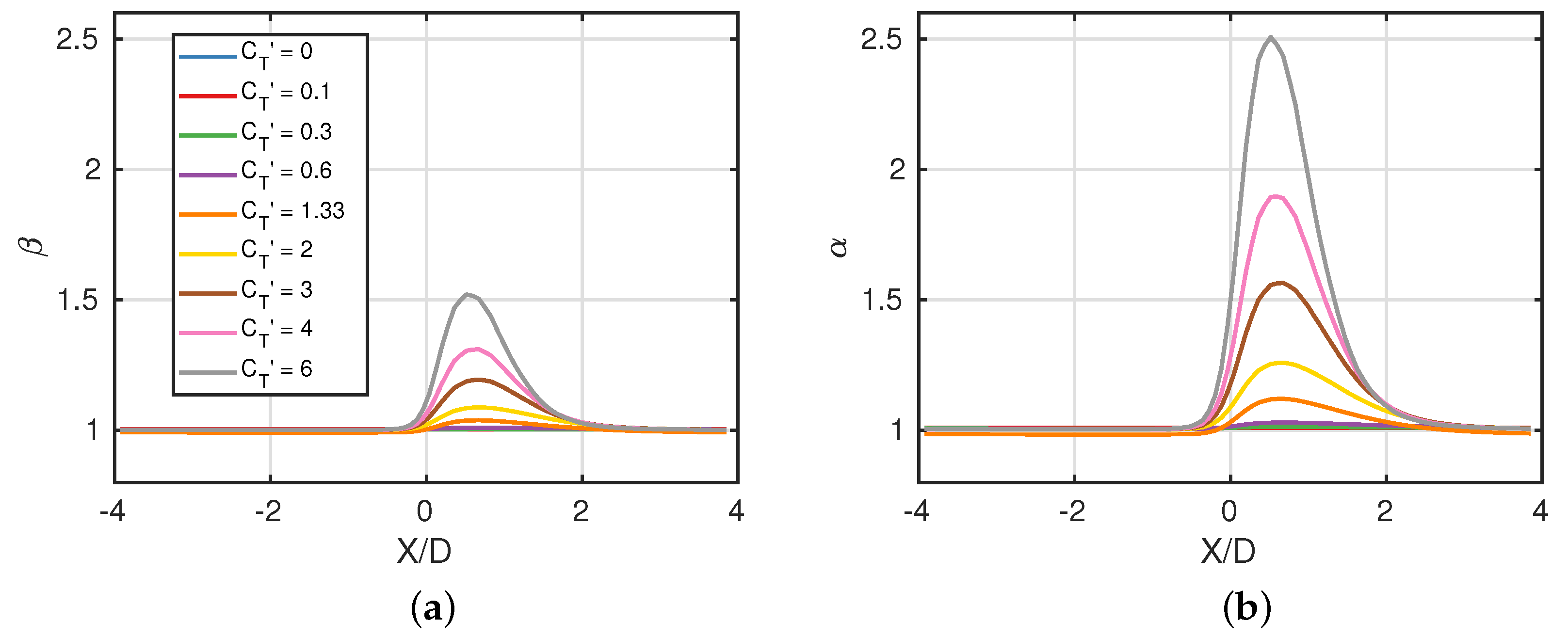
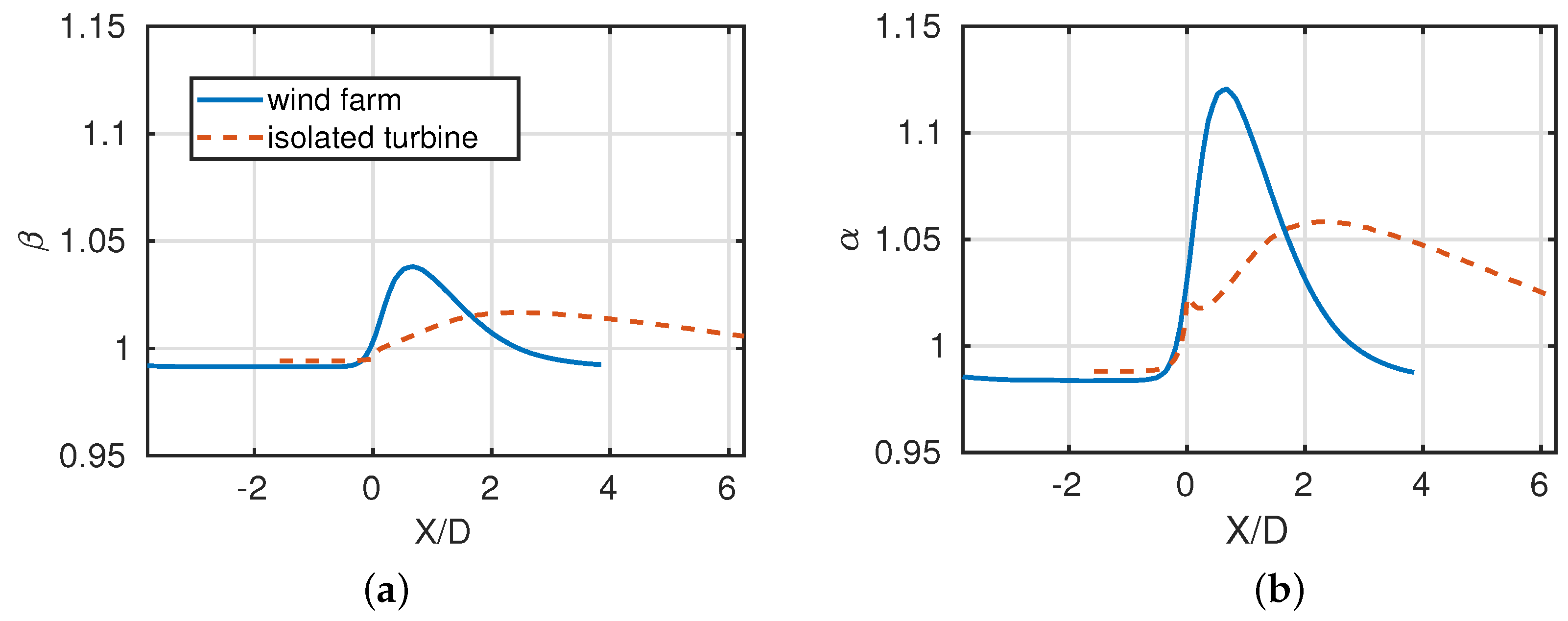
The one-dimensional profiles plotted in Figure 6 do not tell the entire story of the mean flow in the streamtube control volume. For additional perspective, the shape factors α and β , which quantify the non-uniformity of the velocity in the streamtube, are presented in Figure 7. Unsurprisingly, the shape factors are generally close to unity except in the near wake of disks with large C T . As the streamtube intersects the turbine, the velocity field becomes more non-uniform until about one diameter downstream, where it begins to recover towards uniformity. Cases with higher thrust coefficient depart further from unity because they create a larger velocity deficit behind the turbine. For much of the length of the streamtube, the shape factors are basically constant, even for large C T . This does not mean the velocity is constant, but that the wake has reached a self-similar state as it recovers.
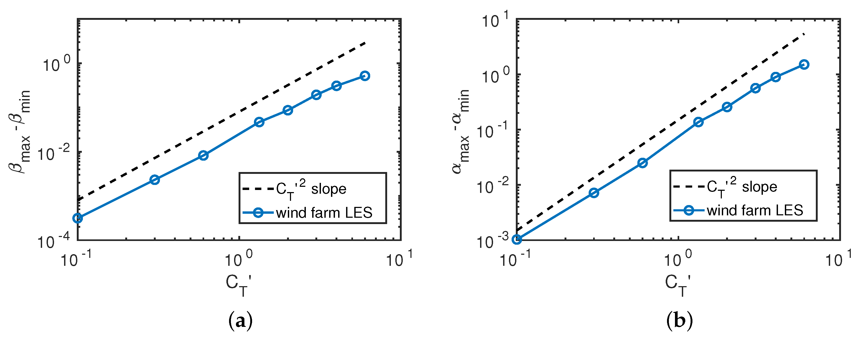
The peak value of both shape factors scales with C T 2 , as shown in Figure 8. For the higher thrust coefficients simulated, the scaling diverges only slightly. This scaling can be predicted using a wake model, such as the lifting line model developed by Shapiro et al. [31]. In this model, the steady-state velocity in the turbine wake is given by
u x U 1 2 a g ( x , y , z )
where a is the induction factor of the actuator disk, and g ( x , y , z ) is a function describing wake spreading, which only depends on the location downstream of the turbine. The shape factor β can be expressed in terms of this velocity:
β = u x 2 u x 2 = 1 4 a g ( x ) + 4 a 2 g 2 ( x ) ( 1 2 a g ( x ) ) 2
Subtracting 1 from β , the right hand side can be simplified.
β 1 = 4 a 2 ( g 2 g 2 ) ( 1 2 a g ) 2
Recognizing that β m i n 1 , and substituting in the definition a = C T 4 + C T results in
β m a x β m i n 4 C T 2 ( g 2 m a x g m a x 2 ) ( 4 + C T ( 1 g m a x ) ) 2
In terms of scaling, this yields
β m a x β m i n C T 4 + ( 1 g m a x ) C T 2
where ( 1 g m a x ) is between 1 and + 1 , based on the functional form of g ( x , y , z ) . Therefore, a scaling of β m a x β m i n C T 2 is predicted by the wake model at small values of C T , with some deviation at higher values depending on the value of g m a x . A similar derivation for α m a x α m i n results in a relationship with more complicated dependence on g m a x , but which still allows for a scaling of C T 2 .
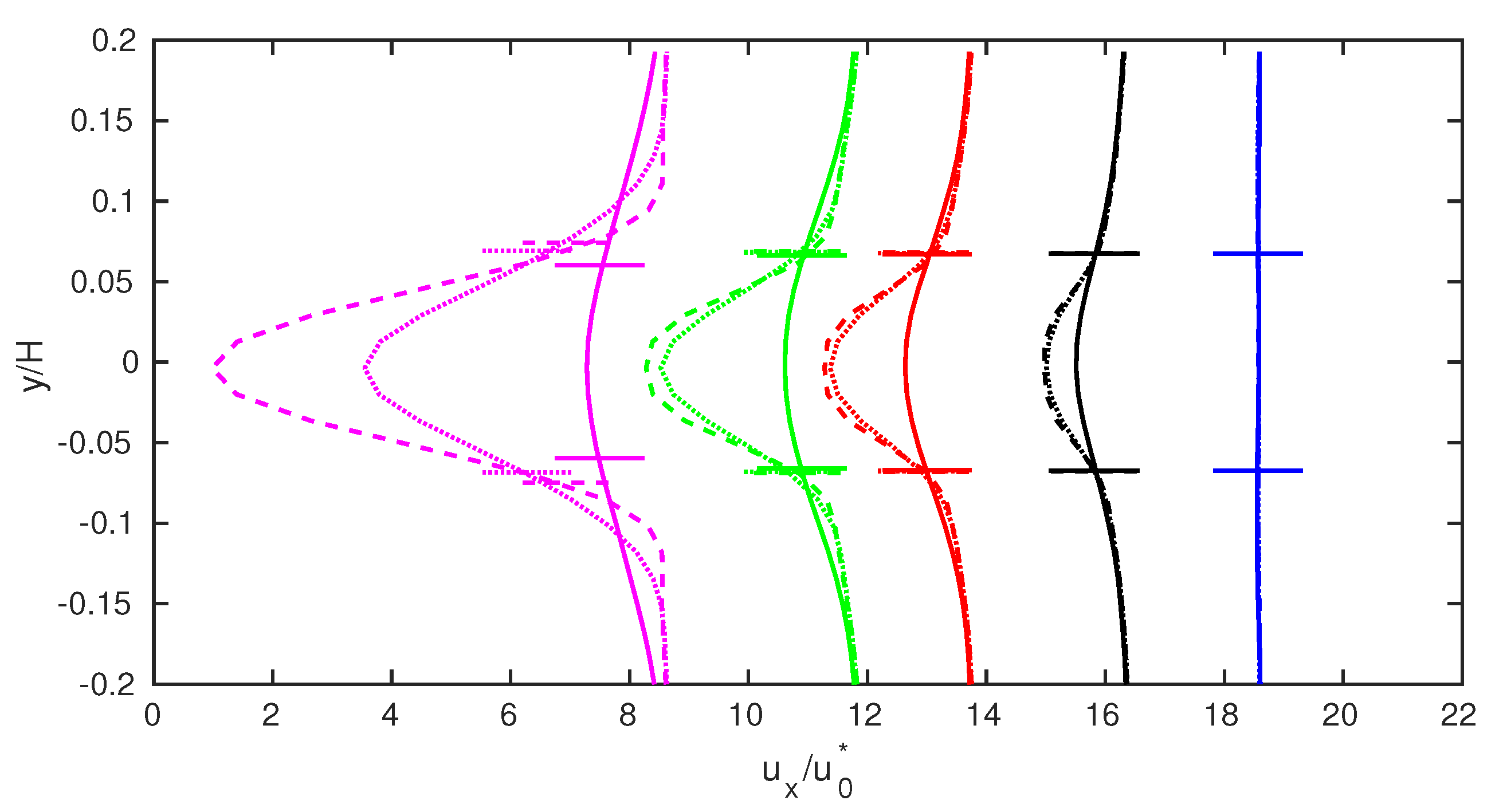
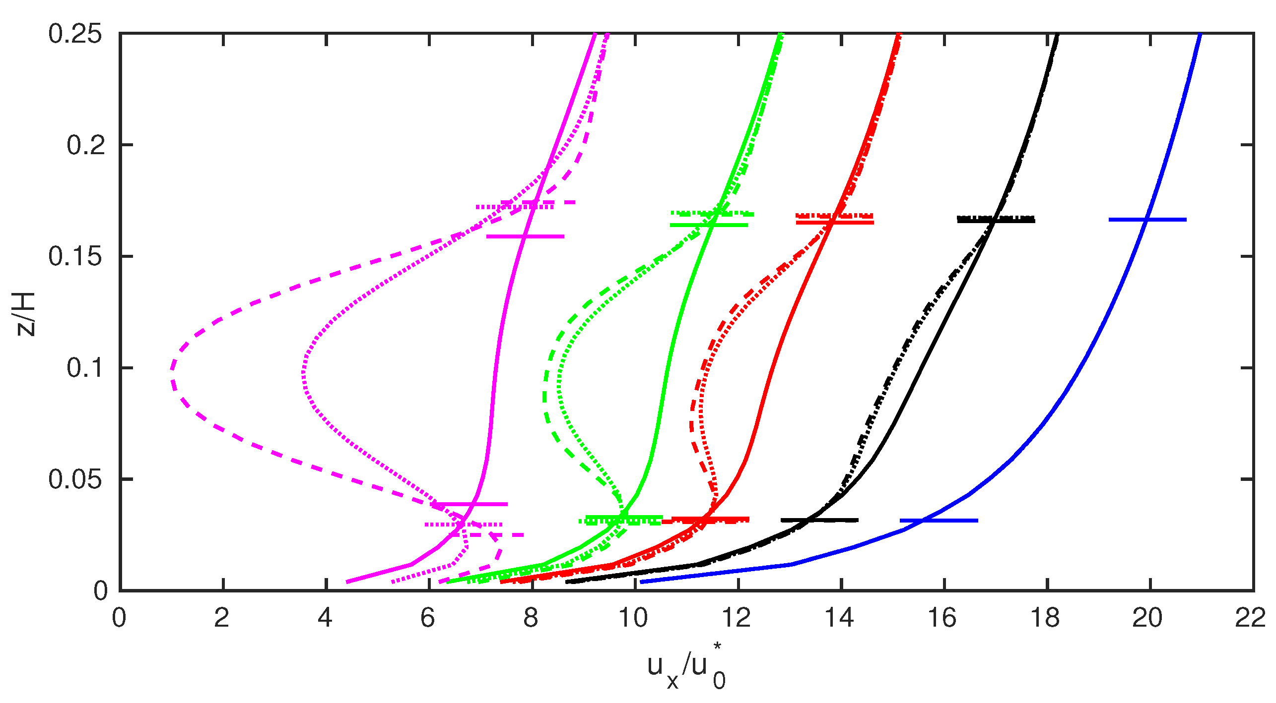
When interpreting the shape factors β and α , it is important to remember that this control volume is larger in diameter than the actuator disk, and so the shape factors may reflect both the faster flow outside the turbine wake and the slower flow inside it, especially in the near wake. The velocity profiles themselves are plotted in Figure 9 and Figure 10. As C T increases, the non-uniformity of the velocity profiles increases dramatically, following the C T 2 scaling shown in Figure 8. Also, as C T increases, the transverse extent of the wake is significantly larger than the local streamtube diameter, even though the streamtube expands more as C T increases. There is also evidence of blockage for non-zero values of C T , where there is some acceleration of the flow outside the streamtube downstream of the turbine.

4.1. Freestream Velocity

In order calculate C T and C P , a freestream velocity U by which to normalize must be chosen. In many experiments and simulations, and in the classical Betz analysis, U is straightforwardly defined as the flow velocity far upstream of the actuator disk. However, this poses a problem when considering infinite wind farms, since there is no “upstream” or “downstream”. Nishino’s [9] approach to this problem is to consider the freestream velocity to be the velocity averaged over the disk location in the flow before turbines are added, and this convention is used in the present work. To make this more precise, using the same terminology as Nishino, U T is defined by an integral of the time-averaged streamwise velocity over the actuator disk area:
U T = d i s k u ¯ x ( y , z ) d A A T
If U T is computed at the disk location in a flow without turbines, the result is U T 0 , where the subscript 0 refers to the case without turbines. In this study, U T 0 is treated as the freestream velocity:
U = U T 0
This definition of U naturally includes any non-uniformity in the freestream velocity.

4.2. Effect of C T on Budget Terms

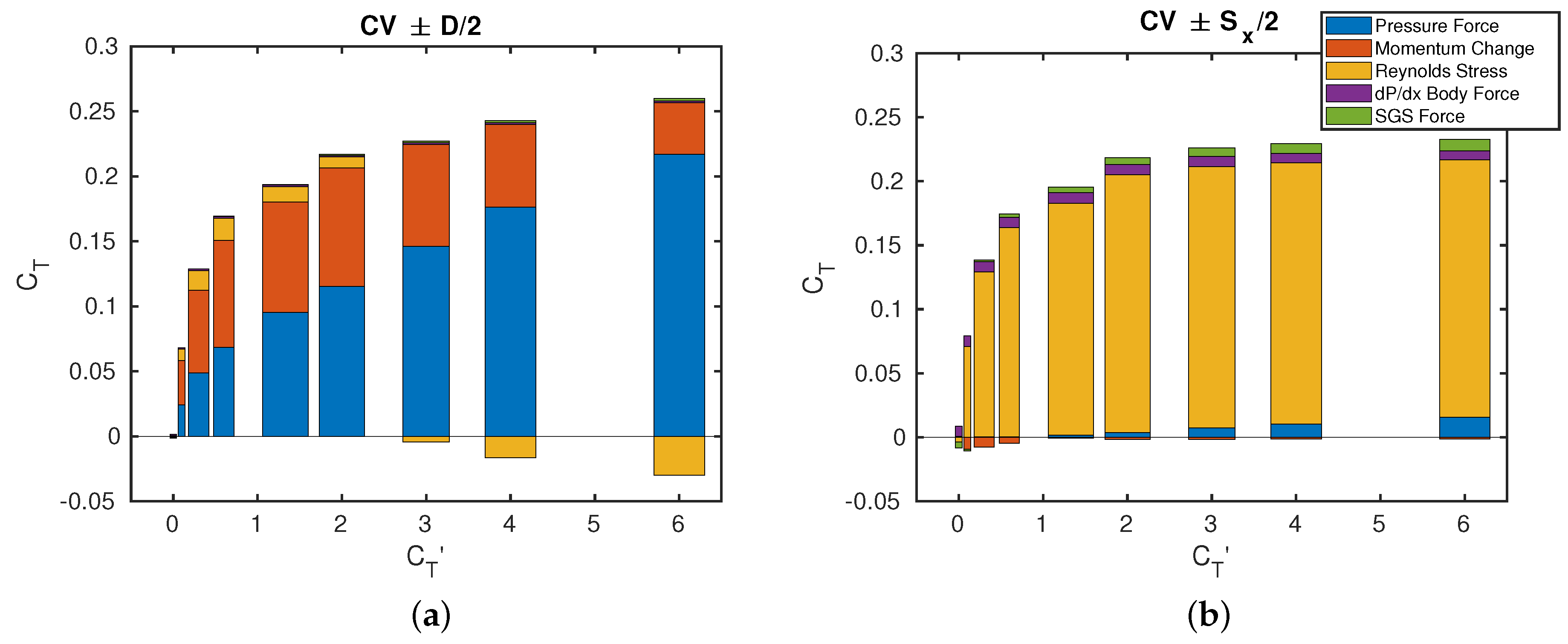
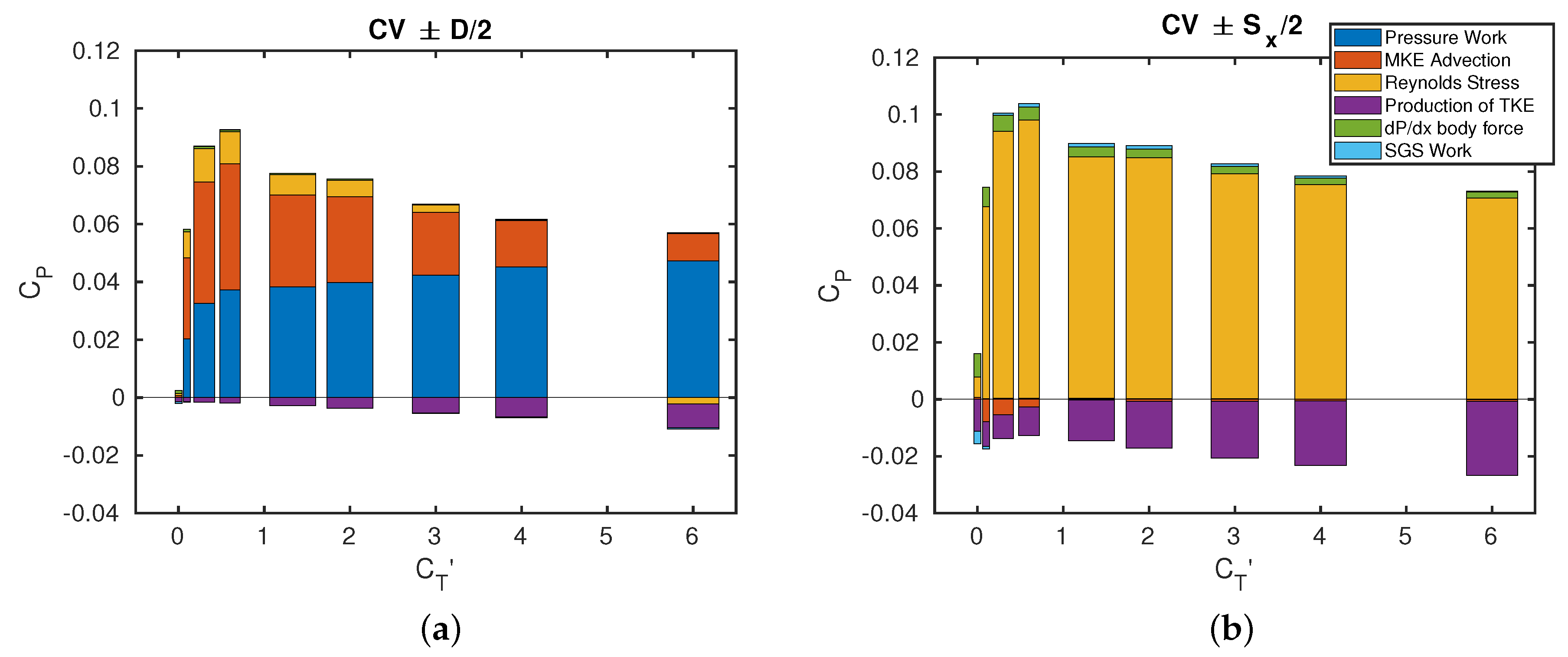
Two important metrics for wind farm design are the overall values of thrust coefficient C T and power coefficient C P for the wind farm. These can be computed directly from LES data by integrating Equations (5) and (9) over the entire wind farm domain. Values of C T and C P can then be compared for different values of C T , but this provides little insight into the physical processes underlying the trends in these values. The expressions for thrust and power coefficient derived from the energy and momentum budgets for the streamtube (Equations (7) and (10)) are useful for this purpose. In Figure 11, the integrated momentum budget in terms of C T is presented as a function of C T . In Figure 12, the energy budget is presented in a similar way. In each case two control volumes are used. “CV ±   D / 2 ” refers to a streamtube that extends upstream and downstream half a turbine diameter, comprising 6 grid points in the streamwise direction. “CV ±   S x / 2 ” refers to a streamtube that extends upstream and downstream half the spacing between turbine rows, encompassing 48 grid points in the streamwise direction. Because of the limitations of numerical integration and statistical convergence, the values of C T and C P computed using the different control volumes are not exactly equal, nor are they equal to C T and C P calculated directly. However, these discrepancies are small, and they are detailed in Appendix A. Both control volumes contain the actuator disk, so both sum to nearly the same value, but the distribution among terms is different. This draws attention to the fact that locally, a wind turbine is a device for harvesting mechanical energy from the wind, but on a large scale, the wind farm relies upon the work done by Reynolds stresses, which re-energize the wind turbine wake.
As before, positive terms in the budget are sources, and negative terms are sinks. Figure 11 shows that as C T increases, the pressure force exerted by the turbine increases monotonically. The momentum extraction increases up to a point, but then begins to decrease due to the blockage effect seen in Figure 9 and Figure 10, as well as the overall slowdown in the flow. This trade-off causes C T to level off for large values of C T . Also, for higher thrust coefficients, the Reynolds stresses actually remove momentum from the control volume just around the wind turbine. This is due to the u x u x ¯ x term. The other terms, which correspond to turbulent stresses due to shear from the top and sides of the streamtube, are always positive when integrated over the streamtube. At all thrust coefficients, the u x u x ¯ x term is negative in the near wake of the wind turbine, but it is severe enough at high thrust coefficients to affect the budget for the small CV chosen here. In other words, the actuator disk causes a local decrease in both the mean and the rms streamwise velocity. The body force and sub-grid scale force remain small compared to the other terms for all C T 0 . For the larger streamtube, the Reynolds stresses are the primary contributor to the turbine force budget. When C T = 0 , this term is negative, which is expected for a standard channel flow. The turbines are in the log layer, where the Reynolds stress balances the stress due to the “ d P / d x ” body force.
Figure 12 shows that as thrust coefficient is increased, pressure work increases, but more slowly than the pressure force, due to blockage and slowdown in the mean flow. The contribution from MKE advection peaks for lower values of thrust coefficient than the momentum change term in the C T budget for the same reason. In the larger streamtube CV, the maximum C P results when the work done by Reynolds stress on the surface of the streamtube is maximized. Also, more MKE is lost to the production of TKE as thrust coefficient increases. The MKE budget for the larger streamtube highlights that the turbine power largely comes from the energy flux due to Reynolds stresses, and that some fraction of that energy is lost into production of TKE. This echoes the analysis of horizontally averaged MKE budgets [11,23]. These results are also consistent with experimental evidence that TKE production and dissipation increase in wind turbine wakes [13,32].

4.3. Actuator Disk with Uniform Turbulent Inflow

It is instructive to compare the wind farm results to the more idealized case of an isolated actuator disk interacting with an un-sheared turbulent freestream wind. The data for this comparison comes from a high-resolution LES study of the interaction of homogeneous isotropic turbulence with a single actuator disk performed by Ghate et al. [24] (case 10) using the same code as the present study. The local thrust coefficient in this study was C T = 1.33 . The horizontal and vertical boundary conditions are periodic, and for the streamwise boundary conditions, a fringe region is used so that periodic boundary conditions can be applied. In the fringe region, the flow is forced based on a concurrent simulation of homogeneous isotropic turbulence.
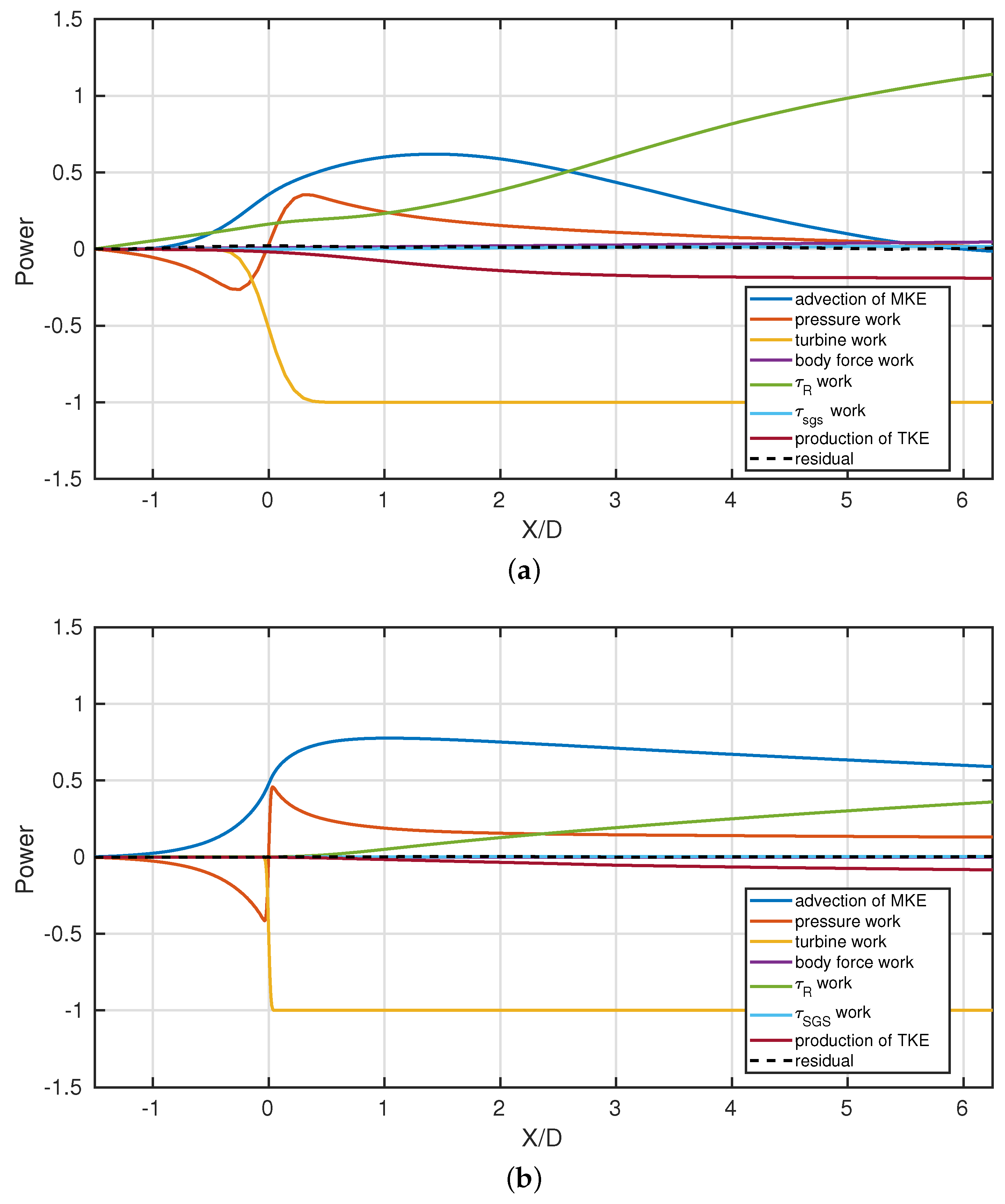
The streamtube is initialized as 1.018 D to capture 99% of the turbine force. This diameter is smaller than the one used in the wind farm cases because the grid resolution was much finer than in the present study. To compare the terms in the energy budget between the isolated turbine and wind farm cases, it is useful to look at the cumulative MKE budget, which is created from the curves in Figure 5 by starting at a point upstream of the turbine and integrating the area under them to a chosen point downstream. This integrated budget is shown in Figure 13, comparing the isolated turbine data to the wind farm data with the same local thrust coefficient, C T = 1.33 . In both cases, each term in the budget has been normalized so that the magnitude of the turbine work term is equal to 1 at the end of the CV.
For the isolated turbine, the terms in the classical streamtube analysis (pressure work, mean advection, turbine work) dominate until x / D 0.5 . After that, turbulence from the growing shear layers begins to add energy back to the wake via Reynolds stresses, and a small amount of mean kinetic energy is lost into turbulent kinetic energy. The wind farm energy budget shows qualitatively similar behavior in the vicinity of the turbine, although the turbine force and pressure drop are less sharply resolved, due to the coarser resolution used. In the wind farm case, the Reynolds stresses acting on the streamtube add energy throughout its length, especially after x / D 1 . Production of TKE is also more significant in the wind farm wake. Finally, the pressure and MKE advection terms return to zero in the wind farm, due to periodicity. For the isolated turbine, pressure does not decay down to the same value as upstream, in contrast to the Betz theory, because the domain has finite streamwise extent and the fringe region does not enforce streamwise periodicity in the pressure field.
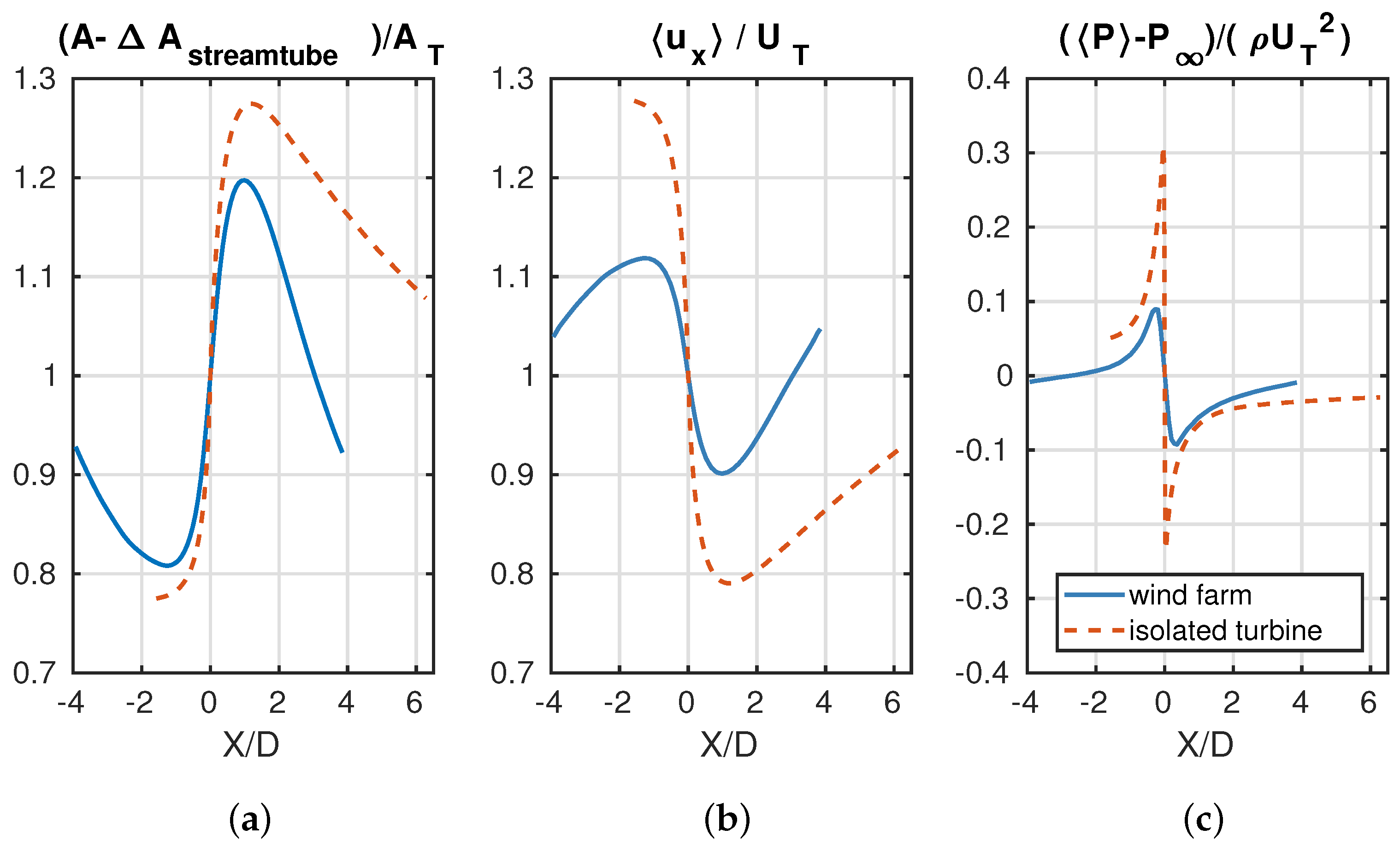
Another instructive comparison can be made by considering streamtube area, velocity, and pressure, shown in Figure 14. As expected, the streamtube expands due to the actuator disk, but it also begins to contract due to turbulent mixing in the wake. However, the streamtube expands more and shrinks more slowly in the isolated case than in the wind farm. This happens because the turbulence which causes wake recovery is different in the two cases. For the isolated turbine, homogeneous turbulence from the inflow and turbulence from the developing shear layers act to add momentum to the wake. In the wind farm, the turbulence of a fully developed channel flow transports momentum much more rapidly, so that the velocity deficits in the wind farm are smaller than in the isolated case. Wu and Porté-Agel [33] have observed that an increase in inflow turbulence intensity accelerates wake recovery, which is consistent with the difference in wake recovery observed here.
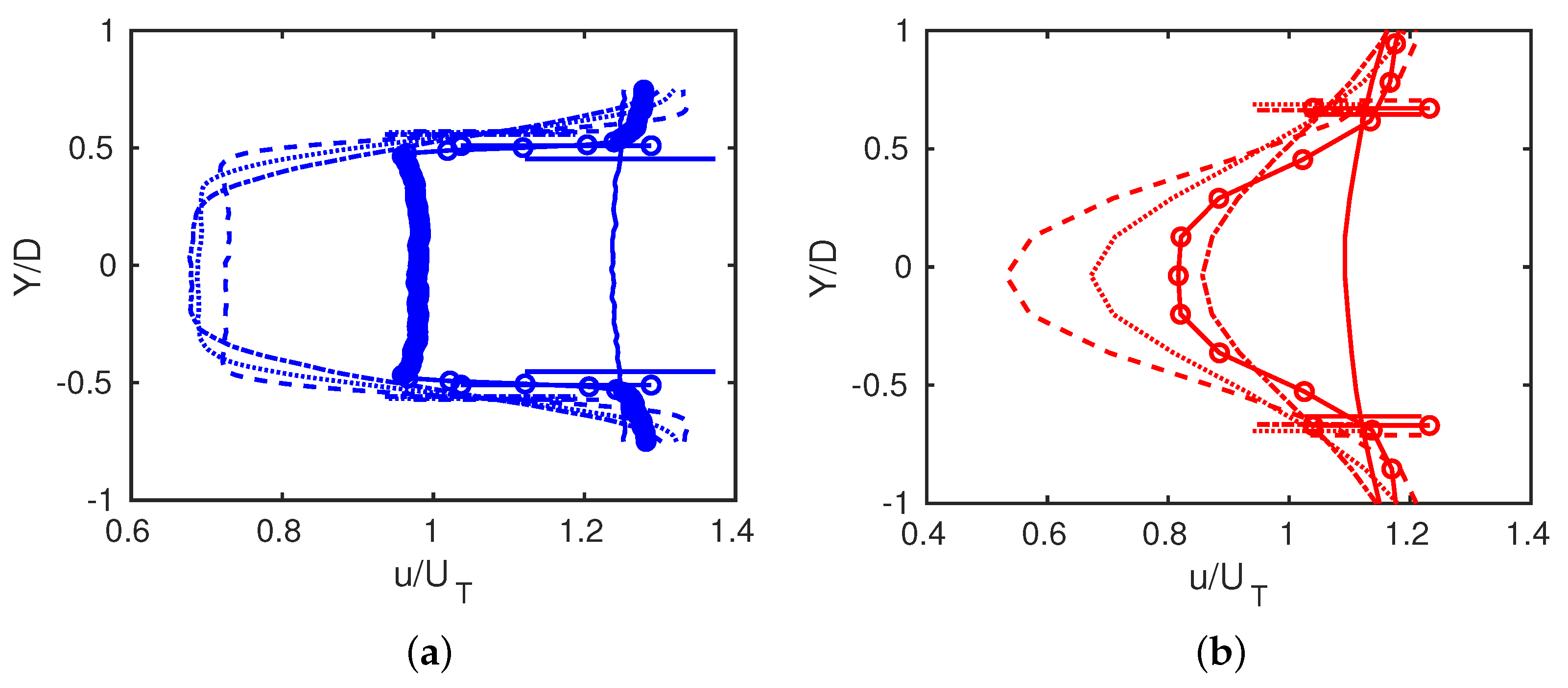
The shape factors for the uniform inflow case and wind farm case with the same thrust coefficient are shown in Figure 15. Velocity profiles for the same cases are shown in Figure 16. The non-uniformity in the velocity profile is less intense for the isolated turbine, but persists much farther downstream than the wind farm cases. The later peak and downstream persistence is explained by the slower rate of turbulent mixing in the wake and slower velocity deficit recovery. The fact that the peak in shape factor is lower may have to do with the way the streamtube is initialized. Because the streamtube is constructed to capture 99% of the force exerted on the flow, it is larger relative to the turbine when a coarser grid is used, since the force is smeared over the grid for numerical stability. Immediately behind the turbine, the larger streamtube therefore contains faster fluid outside the wake.
C T and C P calculated for the isolated turbine are presented in Table 2, along with the wind farm data for the same local thrust coefficient. Interestingly, the power coefficient for the isolated turbine is higher than the value predicted by the Betz theory. This can be explained by the fact that “isolated” turbine is really in a periodic array in the y-z plane, so that the expansion of the streamtube around the turbine is limited by the presence of other turbines. The blockage effect can be estimated based on the ratio of disk area to domain area [4]. For the setup used by Ghate et al., the Betz limit for C P is multiplied by a factor of 1.18. While C T = 1.33 is not necessarily the optimal local thrust coefficient, this suggests that the confinement effect is sufficient to account for the increased C P .

5. Discussion

The numerical simulations in this work have allowed a detailed examination of the momentum and energy budgets of a particular wind farm layout across a wide range of local thrust coefficients. In this section, the effect of shear is examined, and the LES results are compared to the model of Nishino [9]. Finally, Nishino’s model is used to predict how the trade-offs examined here in detail for one layout generalize to other wind farm layouts.

5.1. Effect of Shear

One factor which differentiates the wind farm from the idealized streamtube analysis is a non-uniform inflow velocity in the atmospheric boundary layer. Chamorro and Arndt [6] derived a correction to the Betz limit considering non-uniform inflow for an isolated actuator disk. They found that the Betz-predicted C P is modified by a factor of α 2 β , where α and β have the same definitions used in the present work. Using the values plotted in Figure 7, the influence of non-uniform inflow can be estimated. The shape factors α and β should be evaluated upstream of the the turbine, in the “freestream”. Whether “freestream” is interpreted as the region upstream of the turbine, or in keeping with the Nishino theory, as the flow without turbines, the conclusion is the same. In the wind farm data upstream of the turbine, α [ 0.984 1.009 ] and β [ 0.991 1.003 ] , so the effect of shear on the power coefficient in these simulations is small. C P is modified by at most 3.5 % . Chamorro and Arndt reached a similar conclusion by considering scenarios with realistic roughness heights and turbine parameters.

5.2. Prediction of C T and C P Using Nishino’s Model

Using the model developed by Nishino, the values of C P and C T can be predicted based on the simulation input parameters. Nishino uses both a turbine velocity U T (Equation (17)) and a “farm layer velocity” U F in the model. The farm layer velocity U F is defined based on an integral of the horizontally and time-averaged velocity from the ground up to a height H F , the “farm layer height”. H F is defined implicitly by requiring that U F 0 = U T 0 , where the subscript 0 refers to the flow before turbines are added.
U F = 0 H F 0 D S y 0 D S x u x ¯ d x d y d z H F D 2 S x S y
In very sparse wind farms, the definition of U F limits to U F 0 , which by construction ensures that it limits to U T 0 . The foundational assumption of Nishino’s model is that U F in the wind farm setting is analogous to U in the isolated turbine Betz analysis. A consequence of this is that U T U F 4 4 + C T , from which a formula for C P can be derived:
C P N i s h i n o = C T U F U F 0 3 4 C T + 4 3
Since C T is a characteristic of the individual wind turbines, the accurate prediction of C P in Equation (20) boils down to accurately predicting U F U F 0 , which is a property of the entire wind farm, depending on the farm layout and the flow without turbines. Nishino calculates U F U F 0 by using a force balance between the body force driving the flow, the turbine thrust, and the wall shear stress τ w . Since τ w is not known a priori, Nishino proposes τ w τ w 0 = ( U F U F 0 ) γ , where γ is an empirical constant. There are many models which could be used for τ w , including the top-down model of Calaf et al. [20], which is included here for comparison with Nishino’s suggestion. The results of the LES, along with the predictions based on Nishino’s model, are shown in Figure 17. The agreement in trends is good, and could be improved with suitable tuning of the parameter γ . The wakes of other turbines cause an overall reduction in C T and C P , but turbulent momentum transport and wake recovery make the peaks in these curves flatter than the Betz prediction. At very high values of thrust coefficient, the results from LES begin to show greater disagreement with Nishino’s model, which underpredicts the observed thrust and power. Fortunately, these thrust coefficients are extreme, so Nishino’s model remains useful.
From the streamtube analysis, it is clear that turbulence is important in this flow: turbulent stresses accelerate the turbine wake, allowing it to recover so that the next turbine can extract energy from the wind. Without atmospheric boundary layer turbulence, a wind farm would be limited by viscous diffusion of momentum to far lower values of C P . The fact that Nishino’s model predicts C T and C P effectively using an algebraic model is remarkable, given the dependence of these quantities on turbulent phenomena. It should be noted that the influence of turbulence is accounted for indirectly through the Nishino model in three ways. First, the freestream velocity U comes from a turbulent channel flow simulation. Second, the term U F U F 0 is modeled based on some knowledge of turbulence. Finally, the assumption that the turbine thrust can be estimated by using the farm layer velocity ( U F ) in the classical actuator disk theory seems to rely on enhanced momentum transport due to turbulence. Averaging over this height implies that the momentum in this region will be well-mixed over a streamwise length scale of turbine separation, which only makes sense if there is turbulent momentum transport. Nishino explains that this choice of length scale results in an approximation of the maximum turbine thrust for a wind farm. The maximum would be obtained through a prudent arrangement of the turbines with respect to each other. This seems to imply that if turbines were very densely packed, then the model would break down, since the vertical length scale of mixing required might not match the horizontal length scale of turbine separation. Furthermore, if the vertical length scale of mixing could be increased, that would improve wind farm performance, by speeding up wake recovery.
Recent work by Luzzatto-Fegiz and Caulfield [8] addresses these implicit assumptions of turbulent mixing by considering a three layer turbulent boundary layer for finite size wind farms. Using a momentum exchange coefficient to describe how effectively the wind above a wind farm transports momentum to the wind farm below, they find that this coefficient sets limits on wind farm efficiency. They also indicate that while the momentum exchange coefficient for existing wind farms and finite wind farm LES varies only modestly, increasing it would theoretically increase the maximum efficiency of a wind farm. Increases in momentum exchange might be obtainable with unconventional wind farm design, such as incorporating vertical axis wind turbines [34], or unconventional actuator disk forcing [35]. A greater momentum exchange coefficient would help close the gap between the observed C T and C P curves, and those predicted from classical theory, which is shown in the insets of Figure 17.

5.3. Wind Farm Power Density

Nishino defines a normalized wind farm power density - denoted here as η N
η N = 1 2 ρ C P A T U F 0 3 τ w 0 U F 0 S x S y D 2
Because it takes into account the individual turbine performance ( C P ) and the land area used by each turbine ( A T S x S y D 2 ), η N is a fairer way to compare infinite wind farm performance than C P .
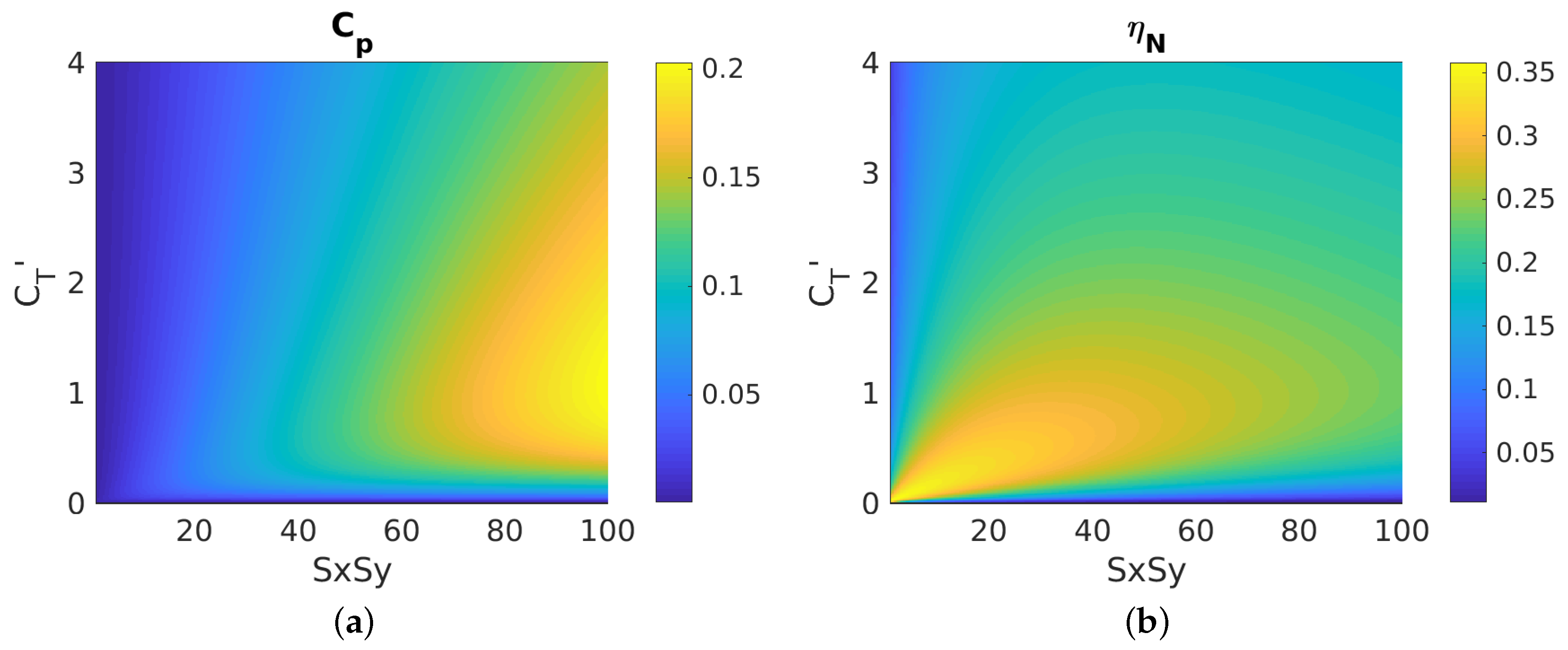
Two examples of the many types of trade-offs that can be explored with Nishino’s model are now described. The model can be used to calculate C P and τ w 0 for a given set of wind farm parameters. U F 0 can be calculated by assuming a logarithmic velocity profile. In Figure 18, C T and S x S y are varied while diameter and turbine hub height ( z h ) are held fixed at D / H = 0.1 and z h / H = 0.1 . This corresponds to a situation where the dimensions of the turbines are known, but the sparsity of the wind farm ( S x S y ) and the turbine thrust ( C T ) are undetermined. From the perspective of an individual turbine, larger spacing is always favorable, as this provides each turbine with the least disturbed inflow, and maximizes C P . However, a closer spacing allows for greater power density ( η N ). Increasing the power density may or may not be economic, depending on the relative costs of land vs. adding additional wind turbines. Regardless of the metric chosen, as the space between turbines increases, a higher value of thrust coefficient is optimal for wind farm performance, and the same thrust coefficient optimizes both C P and η N for a given S x S y . The wind farm LES cases in this study correspond to S x S y 41 , and the C T vs. C P trade-off examined earlier corresponds to a single vertical slice of this contour plot, which has its maximum at C T 0.5 .
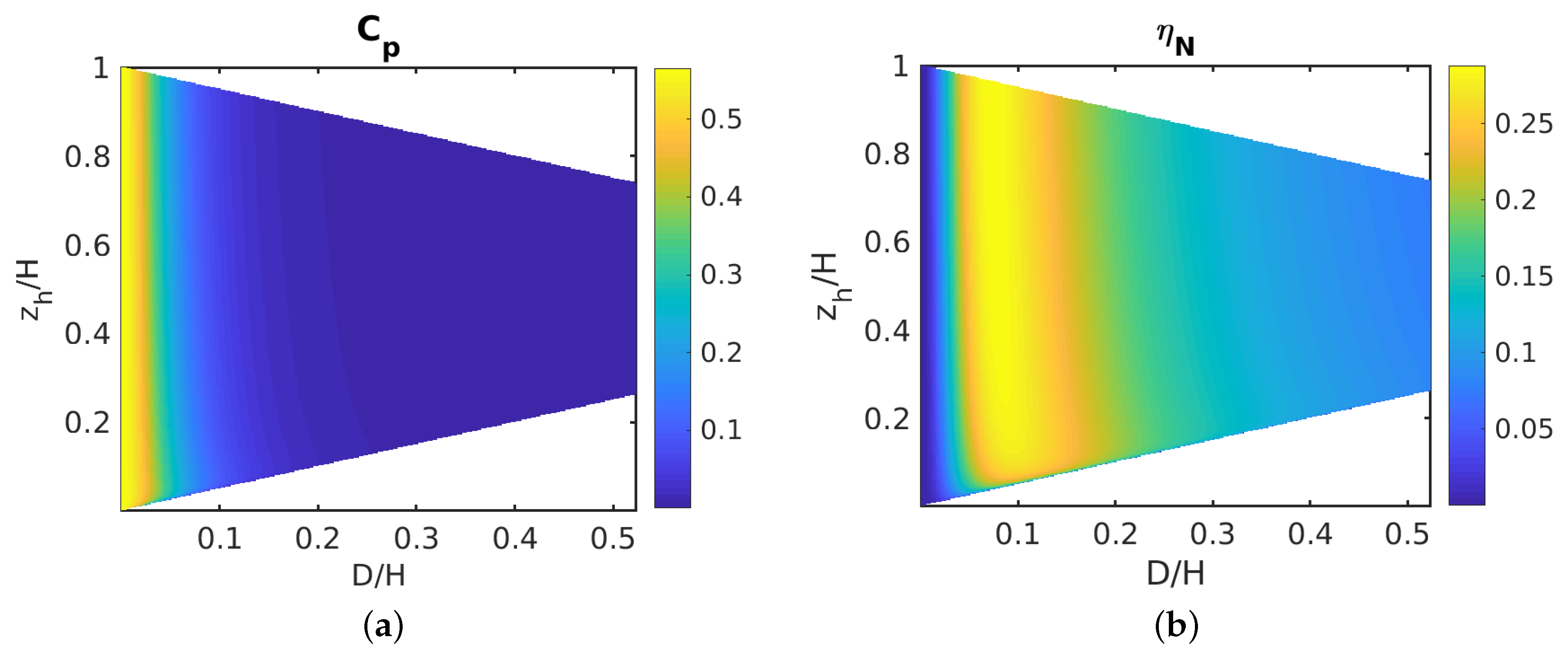
In Figure 19, z h / H and D / H are varied while C T = 1.33 and the wind turbine spacing from the LES cases was used. This corresponds to a scenario where the layout and turbine thrust are set, but the physical dimensions of the turbines are varied. Certain regions of the z h D space are not realizable, since turbines must neither intersect the ground nor adjacent turbines. Within these constraints, for a fixed wind farm spacing, the turbine hub height influences C P very weakly, since U varies with height. Also, a smaller diameter leads to greater C P , for the same reason that increased spacing does: the inflow for each turbine will be less disturbed.
The wind farm power density η N , however, initially increases with increasing diameter and then decreases. This is similar to the trend as thrust coefficient is varied. As the turbine loading (due to D or C T ) increases, more power is generated, but eventually the additional loading slows the flow, decreasing power. The farm power density metric shows a weak dependence on turbine height, implying that changing turbine diameter is a much more effective way to increase the power output of a wind farm than changing the height of the towers. This trade-off is seen in trends in wind farm construction: growth in wind turbine hub heights has been much slower than wind turbine diameters for the past two decades [36].
This simple optimization exercise is included to demonstrate how predictions from an infinite wind farm model (which compare favorably to LES performed here) can be used to explore design trade-offs relevant to wind farm design. Many effects have been neglected, including wind veer with height, atmospheric stratification, and time-varying wind direction and wind speed, all of which could be included in a more detailed analysis. Furthermore, there are other practical considerations for wind farm optimization which have been neglected, such as fatigue loading due to wake interactions [37] and economic considerations such as land and cabling costs [38]. Finally, there are many other promising design variables over which a wind farm can be optimized, which have also been neglected, including wind turbine spacing [39] and turbine control strategies [19,40].

6. Conclusions

This study has presented mean streamwise momentum and mean kinetic energy budgets for a mean streamtube in a periodic array of actuator disks in a channel flow. Inspired by the classical streamtube analysis for steady, irrotational, and one-dimensional flow, the same analysis has been applied to this flow with turbulence, shear, and wake effects. The streamtube analysis was found to be similar in some ways to the Betz results: the streamtube expands as it approaches the turbine, and for a small control volume around the turbine, the energy budget can be explained mostly in terms of pressure work and advection of mean kinetic energy. An alternate perspective considering a larger control volume captures the wind farm effects on an individual wind turbine’s performance. This shows that C P is maximized when the work done by turbulent stresses on the streamtube periphery is maximized, although this must be balanced against minimizing the amount of mean kinetic energy lost to turbulent kinetic energy and eventually dissipated.
The analysis of isolated actuator disk data from Ghate et al. [24] shows that an isolated turbine in a turbulent flow does not experience the same deviation from the Betz limit as the data presented for wind farm LES, since its inflow is not affected by other turbines. This indicates that the modification to the Betz limit in the wind farm setting is due to the wakes of other turbines slowing the flow at hub height, and also to the enhanced mixing and wake recovery in the wind turbine array boundary layer.
The results from LES compare favorably with Nishino’s model, providing additional validation for it. The Nishino model captures the deviations from the Betz limit accurately for values of C T from 0 to 6, although it seems to become less accurate at the high end of this range. To generalize beyond the specific farm layout studied here, a power density metric suggested by Nishino has been used to explore two examples of design trade-offs for wind farms that are described by this model. This highlights the ways in which the optimal thrust coefficient in the infinite wind farm setting is different than for an isolated turbine.

Author Contributions

J.R.W. and S.K.L. conceived the research; J.R.W. conducted analysis; and both authors wrote and edited the paper. All authors have read and agreed to the published version of the manuscript.

Funding

J.R.W. was funded through a Stanford Graduate Fellowship and the TomKat Center for Sustainable Energy at Stanford University.

Acknowledgments

The authors thank Aditya S. Ghate, Akshay Subramanian, and Niranjan S. Ghaisas for developing the LES code used in this study, and for their helpful feedback throughout this project. Access to and use of Ghate’s LES data is also gratefully acknowledged. Michael F. Howland provided helpful feedback on the manuscript. The authors also thank the anonymous referees whose comments have led to many improvements in the paper. The majority of the computing for this study was performed on the Sherlock cluster at Stanford University. The authors thank Stanford University and the Stanford Research Computing Center for providing computational resources and support that contributed to these research results. Some computations were also performed on the Certainty cluster at Stanford University, and the authors acknowledge the resources and support of the Stanford High Performance Computing Center, with partial support from NSF-CBET-1803378.

Conflicts of Interest

The authors declare no conflict of interest.

Abbreviations

The following abbreviations are used in this manuscript:
α shape factor for advection of mean kinetic energy
ainduction factor of actuator disk
Astreamtube cross-sectional area
A T area of actuator disk
ABLatmospheric boundary layer
β shape factor for advection of mean streamwise momentum
γ empirical constant in Nishino’s model
C T thrust coefficient
C T local thrust coefficient
C P power coefficient
CVcontrol volume
Δ A s t r e a m t u b e difference between the area of the actuator disk and the streamtube, at the disk location
Dactuator disk diameter
f i generic body force per unit volume in the i t h coordinate direction
f t u r b i n e streamwise body force per unit volume due to actuator disk
f d P d x streamwise body force per unit volume associated with streamwise pressure gradient
f s g s streamwise body force per unit volume due to subgrid scale stresses
F t u r b i n e streamwise body force due to turbine
g ( · ) generic function
η N wind farm power density in Nishino’s model
Hdomain height
H F wind farm layer height used in Nishino’s model
LESlarge eddy simulation
MKEmean kinetic energy
Ppressure
P atmospheric pressure
ρ fluid density
R e Reynolds number
S i j strain rate tensor
S x streamwise row spacing, normalized by turbine diameter
S y spanwise column spacing, normalized by turbine diameter
τ i j R Reynolds stress tensor
τ i j s g s sub-grid scale stress tensor
ttime
TKEturbulent kinetic energy
u i fluid velocity in the i t h coordinate direction
u 0 * friction velocity in channel flow without actuator disks
u x streamwise velocity
U freestream velocity
U F wind farm layer velocity used in Nishino’s model
U T fluid velocity averaged over actuator disk area
V ˙ volumetric flow rate through stream tube cross section
x a ,   x b streamwise locations that mark start/end of control volume
x i spatial coordinate ( x , y , z )
z 0 , l o roughness height of the domain bottom boundary
z h wind turbine hub height
  ·   ¯ operator denoting averaging over time and ensemble of turbines
· operator denoting averaging over streamtube cross section

Appendix A. Budget Residuals for Wind Farm Simulations

Wind turbine performance metrics C T and C P can be calculated directly from the turbine force and streamwise velocity output from LES, by integrating Equations (5) and (9) over the entire computational domain. They can also be calculated indirectly, by summing the terms on the right hand side of Equations (7) and (10). In addition, different control volumes can be used for this indirect calculation of C T and C P . The accuracy of the indirect method depends on how well closed the budgets are. In Table A1 and Table A2, values of C T and C P computed “indirectly” from various control volumes are compared to those computed directly. The residual between direct calculation and the streamtube control volume method never exceeds 4.4% of the value of C T , or 7.1% of the value of C P .
Table A1. Comparison of C T calculations using different methods. “Turbine Only CV” and “Entire Streamtube CV” are computed by summing the terms on the right hand side of Equation (10). Residuals are shown as a percentage of C T calculated directly from Equation (9), except for C T = 0 , where C T = 0 by definition.
C T C T Equation (9)Turbine Only CVResidualEntire Streamtube CVResidual
0.000.0003-0.0004-
0.10.06980.0681−2.38%0.0687−1.58%
0.30.13260.1289−2.81%0.1308−1.37%
0.60.17200.1694−1.51%0.1701−1.09%
1.330.19740.1938−1.79%0.1949−1.27%
2.00.21390.21701.44%0.21701.47%
3.00.21820.22282.13%0.22462.91%
4.00.23570.2264−3.92%0.2281−3.21%
6.00.24030.2302−4.22%0.2312−3.78%
Table A2. Comparison of C P calculations using different methods. “Turbine Only CV” and “Entire Streamtube CV” are computed by summing the terms on the right hand side of Equation (7). Residuals are shown as a percentage of C P calculated directly from Equation (5), except for C T = 0 , where C P = 0 by definition.
C T C P Equation (5)Turbine Only CVResidualEntire Streamtube CVResidual
0.000.0003-0.0004-
0.10.05800.0566−2.36%0.0570−1.58%
0.30.08800.0854−2.95%0.0867−1.46%
0.60.09240.0907−1.79%0.0911−1.35%
1.330.07730.0747−3.32%0.0752−2.62%
2.00.07160.07190.46%0.07200.60%
3.00.06120.06150.63%0.06211.53%
4.00.05810.0548−5.81%0.0553−4.95%
6.00.04960.0461−7.06%0.0464−6.34%

References

  1. Barthelmie, R.J.; Hansen, K.; Frandsen, S.T.; Rathmann, O.; Schepers, J.G.; Schlez, W.; Phillips, J.; Rados, K.; Zervos, A.; Politis, E.S.; et al. Modelling and measuring flow and wind turbine wakes in large wind farms offshore. Wind Energy 2009, 12, 431–444. [Google Scholar] [CrossRef]
  2. Meneveau, C. Big wind power: seven questions for turbulence research. J. Turbul. 2019, 20, 2–20. [Google Scholar] [CrossRef] [Green Version]
  3. Burton, T.; Jenkins, N.; Sharpe, D.; Bossanyi, E. Wind Energy Handbook, 2nd ed.; John Wiley & Sons: Hoboken, NJ, USA, 2011. [Google Scholar]
  4. Garrett, C.; Cummins, P. The efficiency of a turbine in a tidal channel. J. Fluid Mech. 2007, 588, 243–251. [Google Scholar] [CrossRef] [Green Version]
  5. Wagner, R.; Courtney, M.; Gottschall, J.; Lindelöw-Marsden, P. Accounting for the speed shear in wind turbine power performance measurement. Wind Energy 2011, 14, 993–1004. [Google Scholar] [CrossRef] [Green Version]
  6. Chamorro, L.P.; Arndt, R. Non-uniform velocity distribution effect on the Betz–Joukowsky limit. Wind Energy 2013, 16, 279–282. [Google Scholar] [CrossRef]
  7. Draper, S.; Nishino, T.; Adcock, T.A.A.; Taylor, P.H. Performance of an ideal turbine in an inviscid shear flow. J. Fluid Mech. 2016, 796, 86–112. [Google Scholar] [CrossRef] [Green Version]
  8. Luzzatto-Fegiz, P.; Caulfield, C.c.P. Entrainment model for fully-developed wind farms: Effects of atmospheric stability and an ideal limit for wind farm performance. Phys. Rev. Fluids 2018, 3, 093802. [Google Scholar] [CrossRef] [Green Version]
  9. Nishino, T. Two-scale momentum theory for very large wind farms. J. Phys. Conf. Ser. 2016, 753, 032054. [Google Scholar] [CrossRef]
  10. Takafumi, N. Generalisation of the Two-scale Momentum Theory for Coupled Wind Turbine/Farm Optimisation. In Proceedings of the 25th National Symposium on Wind Engineering, Terni, Italy, 25–28 September 2018. [Google Scholar]
  11. Abkar, M.; Porté-Agel, F. Mean and turbulent kinetic energy budgets inside and above very large wind farms under conventionally-neutral condition. Renew. Energy 2014, 70, 142–152. [Google Scholar] [CrossRef]
  12. Cortina, G.; Sharma, V.; Torres, R.; Calaf, M. Mean kinetic energy distribution in finite-size wind farms: A function of turbines’ arrangement. Renew. Energy 2020, 148, 585–599. [Google Scholar] [CrossRef]
  13. Lebron, J.; Castillo, L.; Meneveau, C. Experimental study of the kinetic energy budget in a wind turbine streamtube. J. Turbul. 2012, 13, N43. [Google Scholar] [CrossRef]
  14. Meyers, J.; Meneveau, C. Flow Visualization using momentum and energy transport tubes and applications to turbulent flow in wind farms. J. Fluid Mech. 2013, 715, 335–358. [Google Scholar] [CrossRef] [Green Version]
  15. Porté-Agel, F.; Wu, Y.T.; Chen, C.H. A numerical study of the effects of wind direction on turbine wakes and power losses in a large wind farm. Energies 2013, 6, 5297–5313. [Google Scholar] [CrossRef]
  16. Yang, X.; Kang, S.; Sotiropoulos, F. Computational study and modeling of turbine spacing effects in infinite aligned wind farms. Phys. Fluids 2012, 24, 115107. [Google Scholar] [CrossRef]
  17. Cortina, G.; Calaf, M.; Cal, R.B. Distribution of mean kinetic energy around an isolated wind turbine and a characteristic wind turbine of a very large wind farm. Phys. Rev. Fluids 2016, 1, 074402. [Google Scholar] [CrossRef]
  18. Abkar, M.; Porté-Agel, F. The effect of free-atmosphere stratification on boundary-layer flow and power output from very large wind farms. Energies 2013, 6, 2338–2361. [Google Scholar] [CrossRef] [Green Version]
  19. Munters, W.; Meyers, J. Dynamic strategies for yaw and induction control of wind farms based on large-eddy simulation and optimization. Energies 2018, 11, 177. [Google Scholar] [CrossRef] [Green Version]
  20. Calaf, M.; Meneveau, C.; Meyers, J. Large eddy simulation study of fully developed wind-turbine array boundary layers. Phys. Fluids 2010, 22, 015110. [Google Scholar] [CrossRef] [Green Version]
  21. Ghate, A.; Subramanian, A. PadeOps GitHub Repository. Available online: https://github.com/FPAL-Stanford-University/PadeOps (accessed on 28 February 2018).
  22. Ghate, A.S.; Lele, S.K. Subfilter-scale enrichment of planetary boundary layer large eddy simulation using discrete Fourier–Gabor modes. J. Fluid Mech. 2017, 819, 494–539. [Google Scholar] [CrossRef]
  23. Howland, M.F.; Ghate, A.S.; Lele, S.K. Influence of the geostrophic wind direction on the atmospheric boundary layer flow. J. Fluid Mech. 2020, 883, A39. [Google Scholar] [CrossRef]
  24. Ghate, A.; Ghaisas, N.; Towne, A.; Lele, S. Interaction of small scale Homogenenous Isotropic Turbulence with an Actuator Disk. In Proceedings of the AIAA SciTech Forum Wind Energy Symposium, Kissimmee, FL, USA, 8–12 January 2018. [Google Scholar]
  25. Stevens, R.J.; Meneveau, C. Flow Structure and Turbulence in Wind Farms. Annu. Rev.Fluid Mech. 2017, 49, 311–339. [Google Scholar] [CrossRef]
  26. Mehta, D.; van Zuijlen, A.; Koren, B.; Holierhoek, J.; Bijl, H. Large Eddy Simulation of wind farm aerodynamics: A review. J. Wind Eng. Ind. Aerodyn. 2014, 133, 1–17. [Google Scholar] [CrossRef]
  27. Calaf, M.; Parlange, M.B.; Meneveau, C. Large eddy simulation study of scalar transport in fully developed wind-turbine array boundary layers. Phys. Fluids 2011, 23, 126603. [Google Scholar] [CrossRef] [Green Version]
  28. Allaerts, D.; Meyers, J. Large eddy simulation of a large wind-turbine array in a conventionally neutral atmospheric boundary layer. Phys. Fluids 2015, 27, 065108. [Google Scholar] [CrossRef] [Green Version]
  29. Munters, W.; Meneveau, C.; Meyers, J. Shifted periodic boundary conditions for simulations of wall-bounded turbulent flows. Phys. Fluids 2016, 28, 025112. [Google Scholar] [CrossRef] [Green Version]
  30. Moin, P. Fundamentals of Engineering Numerical Analysis, 2nd ed.; Cambridge University Press: Cambridge, UK, 2010. [Google Scholar] [CrossRef]
  31. Shapiro, C.R.; Gayme, D.F.; Meneveau, C. Modelling yawed wind turbine wakes: a lifting line approach. J. Fluid Mech. 2018, 841, R1. [Google Scholar] [CrossRef] [Green Version]
  32. Lundquist, J.K.; Bariteau, L. Dissipation of Turbulence in the Wake of a Wind Turbine. Bound.-Layer Meteorol. 2015, 154, 229–241. [Google Scholar] [CrossRef]
  33. Wu, Y.T.; Porté-Agel, F. Atmospheric turbulence effects on wind-turbine wakes: An LES study. Energies 2012, 5, 5340–5362. [Google Scholar] [CrossRef]
  34. Dabiri, J.O. Potential order-of-magnitude enhancement of wind farm power density via counter-rotating vertical-axis wind turbine arrays. J. Renew. Sustain. Energy 2011, 3, 043104. [Google Scholar] [CrossRef] [Green Version]
  35. VerHulst, C.; Meneveau, C. Altering kinetic energy entrainment in large eddy simulations of large wind farms using unconventional wind turbine actuator forcing. Energies 2015, 8, 370–386. [Google Scholar] [CrossRef] [Green Version]
  36. Wiser, R.; Bolinger, M. 2018 Wind Technologies Market Report; Technical Report DOE/GO-102019-5191; U.S. Department of Energy Office of Energy Efficiency and Renewable Energy: Washington, WA, USA, 2019.
  37. Troldborg, N.; Larsen, G.C.; Madsen, H.A.; Hansen, K.S.; Sørensen, J.N.; Mikkelsen, R. Numerical simulations of wake interaction between two wind turbines at various inflow conditions. Wind Energy 2011, 14, 859–876. [Google Scholar] [CrossRef]
  38. Stevens, R.J.A.M.; Hobbs, B.F.; Ramos, A.; Meneveau, C. Combining economic and fluid dynamic models to determine the optimal spacing in very large wind farms. Wind Energy 2017, 20, 465–477. [Google Scholar] [CrossRef]
  39. Meyers, J.; Meneveau, C. Optimal turbine spacing in fully developed wind farm boundary layers. Wind Energy 2012, 15, 305–317. [Google Scholar] [CrossRef] [Green Version]
  40. Howland, M.F.; Lele, S.K.; Dabiri, J.O. Wind farm power optimization through wake steering. Proc. Natl. Acad. Sci. USA 2019, 116, 14495–14500. [Google Scholar] [CrossRef] [PubMed] [Green Version]
Figure 1. Example of streamtube control volume with actuator disk shown in gray. Upstream streamtube sections are plotted in red, and downstream in blue. Spatial axes are normalized by the domain height, H.
Energies 13 01078 g001
Figure 2. Cartoon of the wind farm layout used in this study. The body force driving the flow is aligned with the positive X-direction. Spatial axes are normalized by the domain height, H.
Energies 13 01078 g002
Figure 3. Time-averaged streamwise velocity at turbine hub height for C T = 1.33 . The velocity is normalized by u 0 * , the friction velocity from a channel flow without actuator disks. (a) entire domain. (b) ensemble-averaged flow in sub-domain.
Energies 13 01078 g003
Figure 4. Streamwise momentum equation terms integrated over the streamtube cross-section for C T = 1.33 . Each term is normalized by the total turbine force, such that the integral of the turbine force curve is 1 . X / D = 0 is the location of the actuator disk, and the x-axis extends the length of the separation between turbine rows. The residual is the sum of all other terms.
Energies 13 01078 g004
Figure 5. Mean kinetic energy equation terms integrated over the streamtube cross-section for C T = 1.33 . Each term is normalized by the total turbine power, such that the integral of the turbine power curve is 1 . X / D = 0 is the location of the actuator disk, and the x-axis extends the length of the separation between turbine rows. The residual is the sum of all other terms.
Energies 13 01078 g005
Figure 6. Streamtube properties for all wind farm cases (a) cross-sectional area. (b) mean streamwise velocity. (c) mean pressure. Velocity is normalized by the friction velocity from the no-turbines case ( u 0 * ). P is the hydrodynamic pressure at the top of the domain. Δ A s t r e a m t u b e is the difference between the area of the actuator disk and the streamtube, at the disk location.
Energies 13 01078 g006
Figure 7. Shape factors for all wind farm cases. (a) mean streamwise momentum flux shape factor β . (b) mean kinetic energy flux shape factor α .
Energies 13 01078 g007
Figure 8. Scaling of peaks in shape factor with thrust coefficient. (a) streamwise momentum shape factor. (b) mean kinetic energy (MKE) shape factor.
Energies 13 01078 g008
Figure 9. Streamwise velocity profiles in the horizontal plane at hub height. In each group, solid lines = 1 diameter upstream of turbine, dashed = 1D downstream, dotted = 2D downstream. The groups, in order from left to right, have C T = [ 3.0 ,   0.6 ,   0.3 ,   0.1 ,   0.0 ] . Some cases are omitted for the sake of clarity. Horizontal lines indicate the width of the streamtube at different downstream stations.
Energies 13 01078 g009
Figure 10. Streamwise velocity profiles in the vertical plane at turbine center. In each group, solid lines = 1 diameter upstream of turbine, dashed = 1D downstream, dotted = 2D downstream. The groups, in order from left to right, have C T = [ 3.0 ,   0.6 ,   0.3 ,   0.1 ,   0.0 ] . Some cases are omitted for the sake of clarity. Horizontal lines indicate the height of the streamtube at different downstream stations.
Energies 13 01078 g010
Figure 11. Detailed breakdown of C T budget by term in the momentum budget equation, plotted as a function of as a function of C T , and comparing two different streamtube control volumes. (a) budget breakdown for the small control volume, with streamwise extent of 1 turbine diameter. (b) budget breakdown for the large control volume, with streamwise extent of one row separation.
Energies 13 01078 g011
Figure 12. Detailed breakdown of C P budget by term in the MKE budget equation, plotted as a function of as a function of C T , and comparing two different streamtube control volumes. (a) budget breakdown for the small control volume, with streamwise extent of 1 turbine diameter. (b) budget breakdown for the large control volume, with streamwise extent of one row separation.
Energies 13 01078 g012
Figure 13. Cumulative mean kinetic energy budgets for C T = 1.33 cases. Each term is normalized by the magnitude of the total turbine power. (a) Wind farm and (b) isolated actuator disk. X / D = 0 is the location of the actuator disk. The budget for (a) is constructed by starting with the curves in Figure 5 and integrating from upstream to downstream. The budget for (b) is generated in the same manner using data from Ghate et al. [24].
Energies 13 01078 g013
Figure 14. Comparison of streamtube properties for isolated turbine and wind farm, both with C T = 1.33 . (a) cross-sectional area. (b) mean streamwise velocity. (c) mean pressure. Velocities are normalized by the mean velocity averaged over the turbine face ( U T ). U T is used instead of u 0 * because in the isolated turbine case, there are no wall boundaries. P is the hydrodynamic pressure at the top of the domain. Δ A s t r e a m t u b e is the difference between the area of the actuator disk and the streamtube, at the disk location.
Energies 13 01078 g014
Figure 15. Comparison of shape factors for isolated turbine and wind farm, both with C T = 1.33 . (a) mean streamwise momentum flux shape factor β . (b) mean kinetic energy flux shape factor α .
Energies 13 01078 g015
Figure 16. Comparison of streamwise velocity profiles in the horizontal ( x y ) plane at hub height for C T = 1.33 . (a) isolated actuator disk. (b) wind farm. In each group, solid lines = 1 diameter upstream, circles = at actuator disk, dashed = 1D downstream, dotted = 2D downstream, dot-dash = 3D downstream. Horizontal lines indicate the width of the streamtube at different locations downstream.
Energies 13 01078 g016
Figure 17. (a): C T computed directly from LES data, with predictions from Nishino’s model. (b): C P computed directly from LES data, with predictions from Nishino’s model. The Betz prediction for an isolated turbine is shown in the inset.
Energies 13 01078 g017
Figure 18. (a) Individual turbine power coefficient ( C P ) as a function of local thrust coefficient and turbine spacing, with other parameters held fixed, predicted using Nishino’s model. (b) Wind farm power density ( η N ) as a function of local thrust coefficient and turbine spacing, with other parameters held fixed, predicted using Nishino’s model.
Energies 13 01078 g018
Figure 19. (a) Individual turbine power coefficient ( C P ) as a function of turbine diameter and tower height, with other parameters held fixed, predicted using Nishino’s model. (b) Wind farm power density ( η N ) as a function of turbine diameter and tower height, with other parameters held fixed, predicted using Nishino’s model.
Energies 13 01078 g019
Table 1. Parameters common to wind farm large eddy simulation (LES) cases. S x is the streamwise distance between turbine rows, normalized by the turbine diameter. S y is the spanwise distance between turbine columns, normalized by the turbine diameter. D is the turbine diameter, H is the height of the domain, and z 0 , l o is the roughness height of the lower wall.
Domain (x,y,z)Grid (x,y,z) S x S y #   Turbines z 0 , lo / H D / H
π , π , 1192, 192, 1287.855.2424 10 4 0.1
Table 2. C T and C P computed from LES, along with Betz predictions, for isolated actuator disk and wind farm with C T = 1.33 .
Case C T C T (Betz Prediction) C T (LES) C P (Betz Prediction) C P (LES)
wind farm [present study]1.330.750.200.560.08
isolated turbine [24]1.330.750.800.560.62