Abstract
The exhaust/return-split configuration is regarded as an important upgrade of traditional under-floor-air-distribution (UFAD) systems due to its higher energy efficiency. Moreover, existing studies are mostly focused on the effect of the return vent height on the performance of an UFAD system under cooling conditions. Knowledge of the performance under heating conditions is sorely lacking. This paper presents a numerical evaluation of the performance characteristics of an UFAD system with six different heights of the return vents in heating operation by comprehensively considering thermal comfort, air quality, and energy consumption. The results show that, in the heating mode, the general thermal comfort (predicted mean vote-predicted percentage dissatisfied (PMV-PPD) values) and indoor air quality indices (mean age of air and volatile organic compounds (VOCs) concentration) were greatly improved and energy consumption was slightly reduced with a lower return vent height. Although these were opposite to the findings of our previous study regarding the performance in cooling mode, an optimal return vent height in terms of the comprehensive all-year performance can be recommended. This method provides insight into the design and optimization of the return vent height of UFAD for space heating and cooling.
1. Introduction
In recent decades, an underfloor air distribution (UFAD) system has been spotlighted as a cooling terminal system, due to its energy efficiency and high ventilation performance [1,2,3]. UFAD produces a stratified air flow pattern that takes advantage of the thermal buoyancy that is produced in cooling mode. Hence, UFAD removes heat loads and contaminants from the space more efficiently when compared with conventional overhead mixing ventilation (MV) [4].
Moreover, some studies have been conducted to investigate the performance of UFAD for heating mode. Tae et al. [5] used Energyplus to evaluate the energy performance of the UFAD and MV systems for heating and cooling in the interior zone of an theatre complex. Their study demonstrated that the heating energy consumption for UFAD was lower than that for MV during the winter heating season (from December to January). Hazim and Gan [6] employed the CFD (Computational Fluid Dynamics) method to compare the thermal comfort, air quality, and ventilation efficiency of UFAD and MV systems that are used for heating an office. It was found that the warm air jet of the UFAD impinged on the ceiling and then flowed downward. In contrast, the warm air that is delivered by MV cannot reach the lower spaces easily due to the thermal buoyancy. Therefore, UFAD was more energy and ventilation efficient than MV. ASHRAE [7] also concluded that the UFAD system might provide significant heating saving relative to overhead system. One interesting finding in these two studies [6,7] was that UFAD produced less thermal stratification than MV in heating mode, which was the opposite in cooling mode [8,9,10].
In recent years, an increasing number of studies has been conducted to evaluate the effects of the split return vent on the performance of the UFAD system for cooling mode, since the UFAD system with split return and exhaust vents provided further energy saving potential. For example, Cheng et al. [11] proposed a numerical procedure for predicting the thermal comfort and energy saving for stratified air distribution systems in a large terraced classroom. They revealed that the cooling coil load reduction could be as large as 16.5% of the total space cooling load with separated locations of return and exhaust vents. A numerical study [12] was further performed to investigate the impact of the return vents height (4.8 m–2.3 m) on the energy efficiency of the system in the same classroom. The results showed that the return air temperature was reduced with decreasing return vent height. Fathollahzadeh et al. [13] numerically investigated the effects of six different return heights (0.1 m–4.0 m) on the thermal environment, indoor air quality (IAQ), and energy saving in a large indoor space. They found that the energy saving increased by reducing the location of the return vent from the ceiling down to the floor level, while the thermal comfort and IAQ were negatively influenced. The return air vent was recommended to be positioned at the upper boundary of the occupied zone (1.7 m) for favorable conditions in a large space. Cheng et al. employed the CFD techniques to numerically study the thermal comfort and energy saving of a small office with a UFAD system [14]. Seven return vent location heights (0.3 m–2.6 m) were considered. A lower installation height of the return vent would lead to enhanced energy saving, while it would reversely affect the thermal comfort, according to this study. They recommended that the return vents should be located at the upper boundary of the occupied zone for seating occupants (1.3 m). Likewise, the study by Heidarinejad et al. [15] also revealed that positioning a return air vent at a lower level was beneficial to saving energy, but negative for the thermal comfort and IAQ in a small office. Apparently, most of the studies demonstrated that the optimum height of return vent in a small space was around 1.3 m in order to maintain a balance between the thermal comfort and energy saving [14,15]. Furthermore, in our previous research [16], a series of numerical computations with various height positions (Z = 0.8 m–2.6 m) of the return vents were conducted in order to comprehensively evaluate the effects of the height of return vents on thermal comfort, contaminant removal, and energy efficiency. The results revealed that positing a return vent at a lower level was beneficial for saving energy and a lower CO2 concentration, but it resulted in another larger mean air age (MAA). Thus, the comprehensive height-effects graph (Figure 1) was created to reveal that an optimal return vent height of 1.05 m–1.3 m was recommended in terms of the ACE 0.95 criteria and a preferable CO2 concentration in the breathing zone. However, these UFAD systems with split return and exhaust vents were only evaluated for the cooling mode.
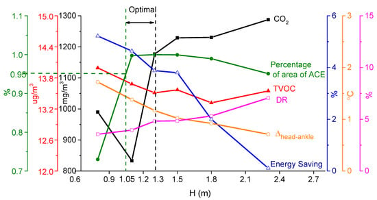
Figure 1.
Comprehensive indices at different height of return air vent in cooling mode.
In practice, it was not feasible to install two separate HVAC systems for heating and cooling in a single building. The HVAC system must serve the building space for the whole year. There have not been detailed studies conducted to evaluate the usability of the UFAD system with exhaust/return-split configuration for both cooling and heating to the author’s best knowledge. The main reason was that the lack of detail and quantitative information of these systems for heating mode. Therefore, a validated CFD model was employed in this study to investigate the effect of the location height of return vents on the energy consumption, indoor thermal comfort, and air quality in the previous domain [16] for heating mode. The objective of this study is to find the optimum height of return vent of an UFAD system for both cooling and heating.
2. Methodology
2.1. Case Description
A room model, which was similar to that of our previous study [16], was built as the computational domain for a comparative study on the heating performance and the cooling one of system. In addition, Park and Chang [17] reported that the UFAD system was ineffective for heating when the large downdraught from the exterior windows could block the buoyancy force above the occupant and stagnant air would occur. It was revealed that care should be exercised to avoid the thermal sink dominant condition in UFAD application for heating, such that UFAD can maintain an advantage over MV in the aspects of energy saving and indoor environment control [6,17]. Hence, the heat sources were designed to be more dominant than the heat sinks in this study.
The dimensions of the full-scale computation domain were 6.0 m. Only half of the model in the X axis direction was investigated for cost-efficiency due to the symmetry of the air flow field (Figure 2). The heating box (0.5 m × 0.4 m × 0.45 m) that was located 0.8 m above the floor represented the internal heat sources, including one occupant and two electrical appliances with total 440 W heat output [18]. The heating box that was used as human representatives released CO2. The rectangular area in the Y wall with dimension of 1 m × 2 m representing a newly painted bookshelf was assumed to emit volatile organic compounds (VOCs). The linear-slot supply diffuser (0.6 m × 0.215 m) was located at the floor level and the exhaust vent (0.5 m × 0.5 m) was located at the ceiling. Six different central heights of the return vent (0.8 m × 0.1 m) were built and they will be tested at X-wall. The target temperature in the occupied zone was 19 °C. 10% of the total air was directly extracted from the exhaust vent. The rest air extracted through the return vent and fresh air both passed the air handling unit and were supplied into the domain via the supply vent. Table 1 summarizes the details of the boundary conditions.
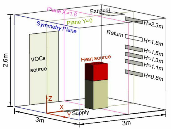
Figure 2.
Schematic illustration of the model room.

Table 1.
Boundary conditions of simulation.
2.2. CFD Model and Validation
The incompressible Navier–Strokes equations, together with the Buossinesq approximation, were applied to calculate the airflow fields. Due to very low concentrations of CO2 and VOCs in the air, the airflow field was assumed not to be influenced by their existence. Gaseous contaminant and the mean age of air (MAA) [19,23,24] were modeled using transportable scalars:
where is the contaminant concentration and represents the velocity component. is the effective diffusion coefficient of the contaminant in the air, is the source term, and is the mean age of air (MAA).
The RNG model was selected for the air turbulence due to its successful prediction of indoor air flow, temperature, and contaminant distribution [25,26]. The Discrete Transfer model [27] was used to simulate the radiation heat, owing to its proven accuracy and high cost-efficiency [28]. CFX 16.0 was adopted as the simulation tool for solving the model equations. The computational domains were discretized using unstructured tetrahedral mesh. The SIMPLE algorithm was selected to solve the velocity-pressure coupling and the second-order discretization method was used to solve all the equations. The highest y+ value that was found in this simulation was 56.14. The standard wall function was used in the RNG model. The grids with total number of cells that ranged from 0.4 million to 2.0 million were tested. It is founded that the maximum percentage error in predicted air flow velocity and temperature was about 0.5% once the mesh elements number was above 1.6 million. Convergence was achieved within 4000 iterations when the residuals of continuity and momentum reach 1 × 10⁻⁴ and the residuals of energy dropped down to 1 × 10⁻⁷.
The experimental data of Wan and Chao [29] were employed in our previous work for model validation. The experimental chamber had the same dimensions and very close layout as the computational model (Figure 2). Different experiments were conducted with air being exhausted from vents that were located in the ceiling and floor, respectively. Table 2 briefly introduced the experimental conditions and more details can be found in [16].
Table 2.
The experiment conditions of Wang and Chao [29].
Figure 3 shows a general agreement between the numerical results and experimental data [29], both in the shape and magnitude of the velocity and temperature. The CO2 and VOCs dispersion can be reasonably extrapolated to be effectively modeled here due to the predominant control of the airflow in the transport and distribution of gaseous contaminants [30,31].
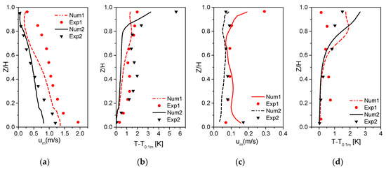
Figure 3.
The comparison of simulated air velocity and temperature against the experimental data: (a,b) Jet centerline; (c,d) Free area (T0.1 m is air temperature at 0.1 m height)
3. Results
3.1. Flow Pattern and Thermal Conditions
Figure 4 shows the air temperature distributions and streamlines on the sectional plane inside the room for heating mode, at H = 0.8 m and H = 2.3 m settings. From Figure 4a,b, it can be found that the supply jet impinged onto the ceiling and spread a certain distance along the ceiling and then dropped downwards the low part of the room for heating mode due to the momentum and buoyance effects. It was similar to the airflow pattern with thermal length scale for the cooling mode, which resulted in relatively uniform temperature distribution [29]. However, the previous finding [16] shows that the supply jets of UFAD system for the cooling mode had a thermal length scale and they would terminate before it reached the ceiling, which led to obvious temperature stratification.
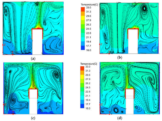
Figure 4.
Temperature and streamline distributions for (a) H = 2.3 m setting at the Plane Y = 0; (b) H = 0.8 m setting at the Plane Y = 0; (c) H = 2.3 m setting at the Plane X = 1.8; and, (d) H = 0.8 m setting at the Plane X = 1.8.
Figure 4a,b show that the thermal plume tended to deflected towards the wall (X = 3) that was installed with the return vents for heating mode due to the downdraught induced by cold air near the wall. It can be seen that the lower the return vents were located, the more the thermal buoyancy flow deflected from the vertical direction. However, the thermal plume rose straight towards the ceiling and was not affected by the location of return vent for cooling mode [16].
In Figure 4c,d, the exterior wall as a cold surface induced the downward flow of air. The thermal plume vacuumed cooler air at a lower zone and distributed it upward due to the upward motion of the warmer air that was developed by the heating boxes. As a result, strong mixing took place between the thermal plume and the downdraft, and then resulted in a comparatively uniform temperature distribution.
Figure 5 demonstrates the velocity and temperature profiles along four vertical lines. Line 1 was the centerline of the floor supply diffuser and the other three lines (2–4) were 0.2 m around the heat source. Figure 5a reveals that the location of the return vent had a negligible effect on the air velocity of the supply jet. It indicated that the short circuit of supply air took place after the supply jet hit the ceiling, and then dropped downwards. From Figure 5b, it can be found that the higher return vent was located, the lower the air temperature along the jet centerline was obtained. This was due to the more significant short circuit of warm supply air by increasing the height of return vent for the heating mode. The findings were different from the previous results for cooling mode [16], where the decreasing location of the return vent caused a short circuit of the cold supply jet and a reduction in momentum of supply air, which led to a lower air velocity and higher temperature of the supply jet.
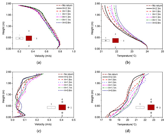
Figure 5.
Effects of the return vent height on the air velocity and temperature profiles: (a,b) along Line 1 (c,d) in the vicinity of heaters.
The location of return vent had a negligible impact on the velocity distribution in the vicinity of occupants, as shown in Figure 5c. It is clear to see that the mean velocity of the occupied zone for each setting was less than 0.1 m/s. It cannot be overlooked that, as the room height level reached approximately y = 2.2 m, the abrupt increase in air velocity around occupants was observed, while the air velocity of the supply jet rapidly decreased (see Figure 5a). This indicates that the supply jet could have been impinging on the ceiling and inducing a horizontal airflow along the ceiling, which protruded into the upper area in the vicinity of occupants. Figure 5d depicts that the shapes of the vertical temperature profiles in the vicinity of heat sources were similar for different settings, and the temperature difference between the floor and ceiling was less than 4 °C in heating mode. This is consistent with the finding of Kennett et al. [32] that thermal stratification decreased in heating mode. It shows that the location of the return vent had a relatively small effect on the temperature profiles and less temperature stratification occurred. Nevertheless, the whole temperature profile was shifted to a lower temperature value with an increase in the height of the return vent, which contributed to the more remarkable short circuit of warm supply air. The finding [16] that the air velocity in the vicinity of occupants was slightly influenced by the height of the return vent for cooling mode was in agreement with the finding for the heating mode. However, a decreased installation height of the return vent led to a lower stratification height and stronger thermal stratification for the cooling mode [13,16].
3.2. Thermal Comfort Evaluation
The predicted mean vote (PMV) and predicted percentage dissatisfied (PPD) have been widely applied to evaluate the general thermal comfort environment of the air distribution system. Fanger [33] combined the following six parameters: air temperature, air velocity, mean radiant temperature, relative humidity, metabolic rate, and clothing insulation into PMV index that can be used to predict the thermal comfort conditions. The PPD, which refers to the percentage of people in a large group who are prone to being thermally dissatisfied with specific thermal environment, is calculated using Fanger’s equation in accordance with the PMV index. These equations were implemented into CFX via CFX Expression Language (CEL). In this study, clothing insulation was fixed to 1.2 for heating mode, the Metabolic rate was set to be 1.6 met, the relative humidity was assumed to be 50%, and the radiant temperature was treated to be the same as the inside wall temperature. Suitable PMV and PPD values were in the range of −0.5 < PMV < 0.5 and PPD < 15%, respectively, according to ISO7730 standards [34].
Figure 6 and Figure 7 illustrate the average PMV and PPD values in the occupied zone from the floor to the room height of 1.8 m for different settings, respectively. For each setting, the value of the PMV index was between −0.4 and −0.64, while the PPD index was between 9.8% and 15.2%. It indicated that the thermal environment was between neutral and slightly cool, which comes to an agreement with Dong’s [17] research. In addition, the results reveal that an increased installation height of the return vent had a negative effect on the general thermal comfort conditions due to the more noticeable short circuit of warm supply air. This was contrary to the findings by [13] that the lower the height of return vent, the more remarkable the short circuit of cold supply air, and the worse the thermal comfort environment for cooling mode. It should be noted that the PMV-PPD indices at H = 1.8 m, H = 2.3 m, and No_return settings exceeded the permitted level that was specified by ISO7730 standards, so they could not meet the occupant’s general thermal comfort needs.
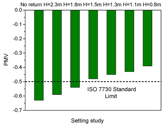
Figure 6.
Predicted mean vote (PMV) index for different settings.
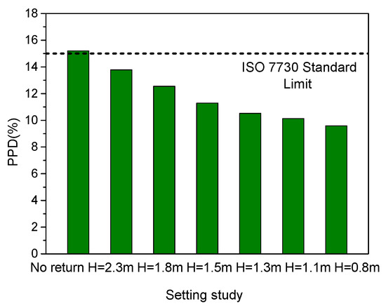
Figure 7.
Predicted percentage dissatisfied (PPD) index for different settings.
The vertical air temperature difference between the ankle (0.1 m) and head (1.1 m) levels and draught comprised two of the major factors in assessing the local thermal discomfort. According to ASHRAE Standard [35], the difference in air temperature from the ankle level to the head level should not exceed 3 °C. Fanger’s equation estimated the percentage of dissatisfied occupants due to draught [34] and it was implemented into CFX via CEL. Standards ISO 7730 [34] suggest that the draught rate (DR) should not be larger than a permissible value of 15% for good air quality.
Table 3 presents the head-to-ankle temperature difference at the three line locations for seven settings. It is clear to see that the vertical air temperature difference for all three lines in each setting was less than the 3 °C limit due to the minor temperature stratification. It is worth noticing that the value of at H = 1.5 m case was obviously smaller than the other six cases. This is due to the fact that the return vent locally extracted the warm air that was generated by the heater before mixing with the air surrounding the head, which is shown in Figure 8. This process led to a reduction in the air temperature at the head zone, which subsequently reduced the temperature difference between the head and ankle levels and improved the local thermal comfort. It was similar to the findings that were revealed by Ahmed et al. [8]. The values of DR for seven settings were generally less than 10% and in an acceptable range, which could be ascribed to the low air velocity (less than 0.1 m/s) of the occupied zone according to Figure 9, as mentioned above. It cannot be overlooked that the DR values in the cases of H = 1.5 m and H = 1.3 m were slightly higher than the values at other five settings. This is because of the comparatively higher velocities for these two cases (see Figure 5b).
Table 3.
Head-ankle temperature difference (°C) for different settings.
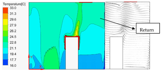
Figure 8.
Temperature and Velocity distribution at the Plane Y = 0 (Case H = 1.5 m).
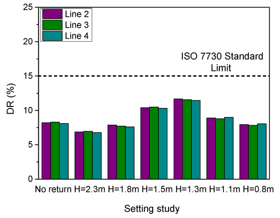
Figure 9.
Draught rate (DR) index for different settings.
3.3. IAQ Evaluation
Two types of indices were used to evaluate the air quality in this study: the local mean air age (MAA) and the air change efficiency (ACE), which quantified the capacity of a ventilation system to renew the air; the concentrations of CO2 and VOCs that quantified the capacity to remove a contaminant. The local MAA represents the time for the supply air to reach a specific point and it reflects the flow characteristics of supply air [36]. Air change effectiveness (ACE) is defined as the ratio between the nominal time and average value of all local mean ages of air at a reference height [37]. The Green Building Council of Australia (GBCA)’ ACE 0.95 criteria [38] suggest that 95% of breathing zone of a sedentary occupant should have an ACE larger than 0.95 when measured in accordance with ASHRAE [39].
Figure 10a presents a typical MAA map in Plane Z = 1.0 for the case of H = 1.5m. The MAA values in the regions closed to the exterior walls were considerably lower, at less than 280 s, as revealed by the graph. It indicates that the exterior wall cooled the supply air bouncing back from the ceiling and it took less time to protrude into the breathing zone. The MAA values in the region near the wall that were installed with the return vent exceeded the nominal time constant of 360 s, which indicated bad air quality for the occupants. This can be attributed to a short circuit of fresh air that is caused by the return vent. Figure 10b compares the MAA data that were extracted from 566 evenly spaced points for each setting at the breathing level. The data points were plotted with 70% transparency to achieve a visualization of their frequency distribution. It was observed that most of the MAA values were between 200 and 425 s for all settings. Moreover, the results reveal that a higher return vent position led to a larger MAA value for the heating mode. This is because more fresh air dropping down from the ceiling would be directly extracted from the room without reaching the breathing zone when the position of return vent was elevated from 0.8 m to the ceiling. Figure 10c shows the vertical profiles of the MAA values in the vicinity of occupants for different settings. The values of MAA continuously decreased with the increase in the heights of the room for each setting. It indicates that the flow characteristics of supply fresh air in heating mode were different from that revealed by Figure 1, in which the supply fresh air was directly delivered to the breathing zone for the cooling mode.
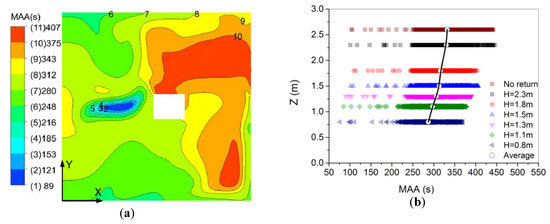
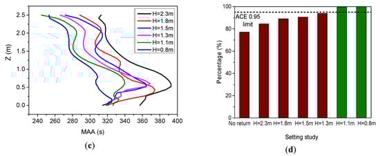
Figure 10.
Mean air age (MAA) values distribution and a air change efficiency (ACE) percentage: (a) MAA value of H = 1.5 m setting at the Plane Z = 1.0; (b) Comparison of MAA values for seven settings at the Plane Z = 1.0; (c) MAA values profile along the room height in the vicinity of occupants; and, (d) ACE percentage in Plane Z = 1.0.
The result was consistent with the frequency distribution of the MAA values for each setting in Figure 10b, according to Figure 10d. It can be concluded that only two settings with the return vent height of 0.8 and 1.1 m satisfied the ACE 0.95 criteria. This was because of the dramatically short-circuit of fresh air in breath zone when the height of return air vents was placed above H = 1.1 m.
Figure 11 shows the air path line that started from the CO2 source, which was used to reflect the path lines of CO2 concentrations that were generated by contaminant sources in this study. According to the results, by changing the position of return vent from H = 2.3 m to H = 0.8 m, more thermal plumes were deflected toward the wall with return vent, which brought more CO2 into the exhaust before it spread into the room. At the same time, the return air with lower CO2 concentration was recycled to the room with a decreasing of the height of the return vent.
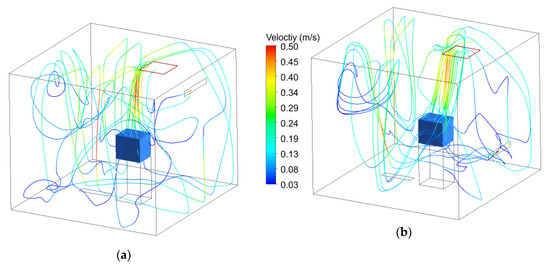
Figure 11.
Air path line from the CO2 source: (a) H = 2.3 m setting; and, (b) H = 0.8 m setting.
Figure 12 presents the frequency distribution of the CO2 concentration. It can be observed that the CO2 concentration distribution was relatively even under different settings and the CO2 concentrations were mostly between 800 mg/m3 and 1300 mg/m3, except for the No_return setting. Based on the results, when the return vent was raised from the 0.8 m to 1.8 m, the CO2 concentration increased slightly. However, further raising the return vent above 1.8m and locating it too close to the ceiling might led to noticeable high CO2 concentration. This was due to the fact that significantly less CO2 was discharged from the exhaust and more CO2 was returned to the room by changing the return vent position from 1.8 m to 2.3 m, as mentioned previously, which added up the CO2 concentration in the breathing zone. Furthermore, when the exhaust used as return was located on the ceiling, a large part of the exhaust air with the highest level of CO2 was returned to the room. The above finding for heating mode was in disagreement with the results that are presented in Figure 1. It showed that, in the cooling mode, the CO2 concentration increased by reducing the return vent height and it was obviously smaller due to the local exhaust when the return vent was located at H = 1.1 m. In Figure 13a, the path line was visualized using the velocity streamline that started from the VOCs source to represent the flow path of VOCs concentrations generated by contaminant sources. It can be observed that the VOCs flowed downwards with the air that was cooled by the cold exterior wall and then mixed with the upward supply air, and finally circulated between the supply vent and the symmetry wall, which corresponded to the flow pattern of supply air that is presented in Figure 3a,b. Therefore, the air in this zone would become stagnant and the VOCs concentration would become high. Figure 13b depicts the VOCs concentration contours in breathing zone for the H = 1.5 m setting. It shows that the VOCs concentrations were higher in the region near the VOCs source and the stagnant zone. It contributed to the dispersal of the VOCs source and the re-circulation in that zone, as mentioned above.
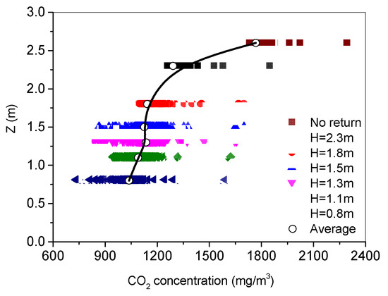
Figure 12.
Comparison of frequency distribution of CO2 concentration for seven settings at breathing level (Plane Z = 1.0).
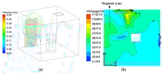
Figure 13.
Air streamline and volatile organic compounds (VOCs) concentration of H = 1.5 m setting: (a) air path line started from VOCs source; (b) distribution of VOCs concentration at the Plane Z = 1.0.
Figure 14 illustrates the frequency distribution of VOCs concentration at the breathing height for seven settings. It can be observed that the majority of VOCs concentrations varied from 6 µg/m3 to 17 µg/m3, except for the No_return setting and the frequency distribution of VOCs concentration was relatively even. This figure implied that increasing the height of return vent slightly affected the distribution of VOCs concentration when the return vent was changed from 0.8 m to 1.8 m. However, the VOCs concentration rapidly increased when the return inlet was further raised above 1.8 m. This is due to the fact that the short circuit of fresh supply air led to an increasing of VOCs concentration in the breathing zone for heating mode when promoting the height of return vent, which was especially obvious in settings of H = 2.3 m and No_return. However, the different results that are indicated in Figure 1 demonstrated that reducing the return vent height from 2.3 m to 0.8 m slightly increased the VOCs concentration for cooling mode, owing to the short circuit of supply fresh air.
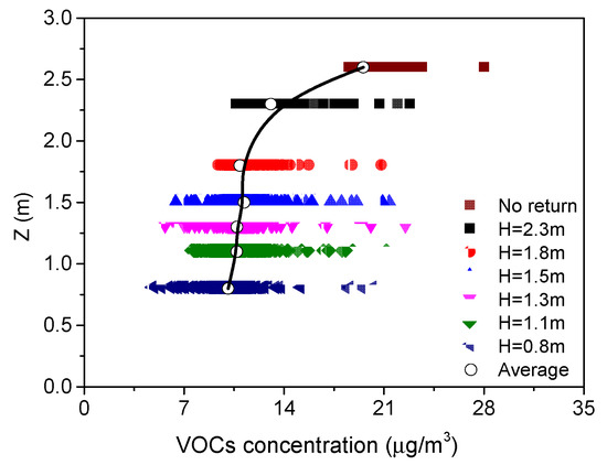
Figure 14.
Comparison of frequency distribution of VOCs concentration for seven settings at breathing level (Plane Z = 1.0).
3.4. Energy Consumption
In the heating season, UFAD systems had an advantage over the MV system, where stratification could occur to the detriment of heating performance [7]. It indicates that there was more obvious stratification in the MV system than that in the UFAD system in heating mode. Therefore, the heating coil load calculation in the UFAD system with the same room set-point air temperature as in the MV system was derived, as following [4,11]:
where (kg/s) is the exhaust air flow rate, (°C) and are the exhaust air temperature of UFAD system and mixing system, respectively, and (°C) is the set-point temperature for the room. It is obvious that an UFAD system, when compared with a MV system, results in decreased heating coil load by the quality of .
Table 4 depicts the influence of the return vent on the energy saving, which was evaluated in terms of . The energy saving increased by raising the height of the return vent from 0.8 m to the ceiling. This was because the return air temperature increased and the exhaust air temperature decreased when the return vent was placed at higher height, which resulted in greater energy saving.
Table 4.
Energy saving for heating coil.
3.5. Overall Performance Assessment
From the above analysis, the position change of return vent has opposite effects on thermal comfort, IAQ, and energy saving; therefore, a comprehensive height-effects graph (Figure 15) was yielded in order to optimize the overall performance of the UFAD system for heating mode. By comparing it with Figure 1, it can be seen that reduced and DR increased by changing the return vent position from 0.8 m to 1.5 m or from ceiling to 1.5 m for heating mode, while a higher return vent height resulted in lower and a larger DR value in cooling mode. Nevertheless, variation in the height of return vents did not have a remarkable impact on the local thermal comfort for both heating and cooling modes, since indices met Standards ISO 7730 and ASHRAE standards, respectively.
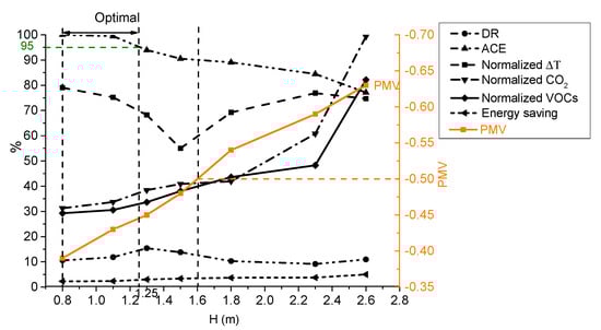
Figure 15.
Comprehensive indices at different height of return air vent in heating mode. Note:; normalized concentration concentration of contaminant in breathing zone; concentration of contaminant in exhaust [8,40].
Figure 15 reveals that the lowest height of return vent (H = 0.8 m) led to the best PMV-PPD value, the lowest CO2 and VOCs levels, and the highest percentage of ACE 0.95, which indicated the best thermal comfort and IAQ performance. However, this same height would result in the smallest amount of heating energy saving. Therefore, it was necessary to trade off the improvement of thermal comfort and IAQ against the decrease in energy saving when determining the proper height of return vent. It can be found that the PMV value exceeded −0.5 when the return vent was set above 1.6 m. In addition, the return vent cannot be located above 1.25 m, due to the requirement of ACE 0.95 criteria. Although energy saving decreased by reducing the height of the return vent, an approximately 0.7% reduction was acceptable when the installation height decreased from 1.25 m to 0.8 m. Based on the comprehensive assessment, positing the return vent between 0.8 m and 1.25 m was advised for the favorable results for heating mode. The lowest return height resulted in the largest quantity of energy saving for cooling mode, as indicated in Figure 1. However, this height (H = 0.8 m) led to the largest PMV value, the highest VOCs level, and exceeding the ACE 0.95 criteria, which indicated worse thermal comfort and IAQ performance. The return vent cannot be set below 1.05 m in terms of the ACE 0.95 criteria. Meanwhile, the concentration of CO2 in the breathing zone was abruptly increased when the return vent was located above 1.3 m. It was recommended that the return air vents should be located between 1.05 m and 1.30 m above the floor for cooling mode through overall evaluation. Thus, it is preferable to install the return vent at a height of between 1.05 m and 1.25 m for the optimum energy saving and better indoor environment in heating and cooling modes.
4. Conclusions
In this study, the performance characteristics of the UFAD system with the various heights of the return vents under heating conditions were numerically investigated by focusing on the thermal comfort, the air quality, and the energy consumption simultaneously. The effects of the return vent height on the overall performance of this system for two modes were taken into account to obtain a good UFAD system with exhaust/return-split configuration for both heating and cooling. The following conclusions are drawn from this study.
(1) Variation in the height of return vent did not have a remarkable impact on the local thermal comfort for two modes. Reducing the height of return vent was beneficial for promoting the general thermal comfort and two of IAQ indices (ACE and VOCs concentration) in heating mode, which was opposite in cooling mode. The ascending return vent return vent had unfavorable effects on the improvement of the other IAQ index as CO2 concentration, for both heating and cooling. Decreasing the height of the return vent led to the reduction of energy saving in heating mode, but it resulted in the increasing of energy saving in the cooling mode.
(2) Therefore, the comprehensive height-effects graph, which adopted thermal comfort, IAQ, and energy saving altogether, was used to design an optimal UFAD system. Accordingly, an optimal return vent height of 1.05 m–1.25 m was recommended to maximize the level of thermal comfort and IAQ with minimum energy input over a whole year.
Although the optimal height of return vent might vary when the heat source distribution, supply air temperature and flow rate were characterized in another way; the method that was utilized in this study can provide a reference for the performance optimization of split-return for space heating and cooling in further research.
Author Contributions
The main contribution was made by Y.F. and X.L.; the other three authors contributed equally. All authors have read and agreed to the published version of the manuscript.
Funding
This research was funded by Natural Science Foundation of Fujian Province (Grant No. 2018J01627 and 2019J01061134), Scientific Research Foundation for the Fujian University of Technology (ID GY-Z17016), and Foundation of Fujian Educational Committee (ID JA0219).
Conflicts of Interest
The authors declare no conflict of interest.
Nomenclature
| ACE | air change effectiveness [-] |
| DR | draught rate [%] |
| IAQ | indoor air quality |
| MV | mixing ventilation [-] |
| MAA | mean air age [s] |
| PMV | predicted mean vote [-] |
| PPD | predicted mean vote [%] |
| UFAD | underfloor floor air distribution [-] |
| VOCs | volatile organic compounds [-] |
| contaminant concentration in returning air (mg/m3) | |
| contaminant concentration in outdoor air (mg/m3) | |
| exhaust air flow rate (kg/s) | |
| velocity component (m/s) | |
| coordination (m) | |
| air density (kg/m3) | |
| contaminant concentration (mg/m3) | |
| source term | |
| exhaust air temperature (°C) | |
| set-point temperature for the room (°C) | |
| age of air (s) | |
| reduced cooling coil load (W) |
References
- Yu, B.H.; Seo, B.-M.; Hong, S.H.; Yeon, S.; Lee, K.H. Influences of different operational configurations on combined effects of room air stratification and thermal decay in UFAD system. Energy Build. 2018, 176, 262–274. [Google Scholar] [CrossRef]
- Yu, K.-H.; Yoon, S.-H.; Jung, H.-K.; Kim, K.; Song, K.-D. Influence of Lighting Loads upon Thermal Comfort under CBAD and UFAD Systems. Energies 2015, 8, 6079–6097. [Google Scholar] [CrossRef]
- Yau, Y.H.; Poh, K.S.; Badarudin, A. A numerical airflow pattern study of a floor swirl diffuser for UFAD system. Energy Build. 2018, 158, 525–535. [Google Scholar] [CrossRef]
- Cheng, Y.; Yang, B.; Lin, Z.; Yang, J.; Jia, J.; Du, Z. Cooling load calculation methods in spaces with stratified air: A brief review and numerical investigation. Energy Build. 2018, 165, 47–55. [Google Scholar] [CrossRef]
- Lim, T.S.; Schaefer, L.; Kim, J.T.; Kim, G. Energy Benefit of the Underfloor Air Distribution System for Reducing Air-Conditioning and Heating Loads in Buildings. Indoor Built Environ. 2011, 21, 62–70. [Google Scholar] [CrossRef]
- Awbi, H.B.; Gan, G. Evaluation of the overall performance of room air distribution. In Proceedings of the 6th International Conference on Indoor Air Quality and Climate, Helsinki, Finland, 4–8 July 1993; Volume 5, pp. 283–288. [Google Scholar]
- UFAD. Guide Design, Construction and Operation of Underfloor Air Distribution Systems; ASHRAE: Atlanta, GA, USA, 2013. [Google Scholar]
- Ahmed, A.Q.; Gao, S.; Kareem, A.K. Energy saving and indoor thermal comfort evaluation using a novel local exhaust ventilation system for office rooms. Appl. Therm. Eng. 2017, 110, 821–834. [Google Scholar] [CrossRef]
- Ameen, A.; Cehlin, M.; Larsson, U.; Karimipanah, T. Experimental Investigation of Ventilation Performance of Different Air Distribution Systems in an Office Environment—Heating Mode. Energies 2019, 12, 1835. [Google Scholar] [CrossRef]
- Alajmi, A.; El-Amer, W. Saving energy by using underfloor air distribution (UFAD) system in commercial buildings. Energy Convers. Manag. 2010, 51, 1637–1642. [Google Scholar] [CrossRef]
- Cheng, Y.; Niu, J.; Gao, N. Stratified air distribution systems in a large lecture theatre: A numerical method to optimize thermal comfort and maximize energy saving. Energy Build. 2012, 55, 515–525. [Google Scholar] [CrossRef]
- Cheng, Y.; Yang, J.; Du, Z.; Peng, J. Investigations on the Energy Efficiency of Stratified Air Distribution Systems with Different Diffuser Layouts. Sustainability 2016, 8, 410. [Google Scholar] [CrossRef]
- Fathollahzadeh, M.H.; Heidarinejad, G.; Pasdarshahri, H. Prediction of thermal comfort, IAQ, and energy consumption in a dense occupancy environment with the under floor air distribution system. Build. Environ. 2015, 90, 96–104. [Google Scholar] [CrossRef]
- Cheng, Y.; Niu, J.; Liu, X.; Gao, N. Experimental and numerical investigations on stratified air distribution systems with special configuration: Thermal comfort and energy saving. Energy Build. 2013, 64, 154–161. [Google Scholar] [CrossRef]
- Heidarinejad, G.; Fathollahzadeh, M.H.; Pasdarshahri, H. Effects of return air vent height on energy consumption, thermal comfort conditions and indoor air quality in an under floor air distribution system. Energy Build. 2015, 97, 155–161. [Google Scholar] [CrossRef]
- Fan, Y.; Li, X.; Yan, Y.; Tu, J. Overall performance evaluation of underfloor air distribution system with different heights of return vents. Energy Build. 2017, 147, 176–187. [Google Scholar] [CrossRef]
- Park, D.Y.; Chang, S. Numerical analysis to determine the performance of combined variable ceiling and floor-based air distribution systems in an office room. Indoor Built Environ. 2013, 23, 971–987. [Google Scholar] [CrossRef]
- Demetriou, D.W.; Khalifa, H.E. Evaluation of distributed environmental control systems for improving IAQ and reducing energy consumption in office buildings. Build. Simul. 2009, 2, 197–214. [Google Scholar] [CrossRef]
- Lin, Z.; Chow, T.T.; Tsang, C.F.; Fong, K.F.; Chan, L.S.; Shum, W.S.; Tsai, L. Effect of internal partitions on the performance of under floor air supply ventilation in a typical office environment. Build. Environ. 2009, 44, 534–545. [Google Scholar] [CrossRef]
- ANSI/ASHRAE. Ventilation for Acceptable Indoor Air Quality; Standard 62.1-2010; ASHRAE: Atlanta, GA, USA, 2010. [Google Scholar]
- Ng, L.C.; Musser, A.; Persily, A.K.; Emmerich, S.J. Indoor air quality analyses of commercial reference buildings. Build. Environ. 2012, 58, 179–187. [Google Scholar] [CrossRef]
- China Architecture. Design code for heating ventilation and air conditioning of civil buildings. In National Standard of the People’s Republic of China; GB 50736-2012; China Architecture & Building Press: Beijing, China, 2012. [Google Scholar]
- Lin, Z.; Chow, T.T.; Tsang, C.F.; Fong, K.F.; Chan, L.S. CFD study on effect of the air supply location on the performance of the displacement ventilation system. Build. Environ. 2005, 40, 1051–1067. [Google Scholar] [CrossRef]
- Kobayashi, N.; Chen, Q.Y. Floor-supply displacement ventilation in a small office. Indoor Built Environ. 2003, 12, 281–291. [Google Scholar] [CrossRef]
- Horikiri, K.Y.Y.; Yao, J. Modelling conjugate flow and heat transfer in a ventilated room for indoor thermal comfort assessment. Build Environ. 2014, 77, 135–147. [Google Scholar] [CrossRef]
- Li, X.; Tu, J. Evaluation of the eddy viscosity turbulence models for the simulation of convection–radiation coupled heat transfer in indoor environment. Energy Build. 2019, 184, 8–18. [Google Scholar] [CrossRef]
- Ansys Inc. Ansys CFX-Solver Theory Guide (Release 15.0); Southpointe: Canonsburg, PA, USA, 2013; Volume 15317. [Google Scholar]
- Li, X.; Yan, Y.; Tu, J. Evaluation of models and methods to simulate thermal radiation in indoor spaces. Build. Environ. 2018, 144, 259–267. [Google Scholar] [CrossRef]
- Wan, M.P.; Chao, C.Y. Numerical and experimental study of velocity and temperature characteristics in a ventilated enclosure with underfloor ventilation systems. Indoor AIR 2005, 15, 342–355. [Google Scholar] [CrossRef]
- Zhuang, R.N.; Li, X.; Tu, J. An energy saving ventilation strategy for short-term occupied rooms based on the time-dependent concentration of CO2. Int. J. Vent. 2015, 14, 39–52. [Google Scholar] [CrossRef]
- Zhuang, R.N.; Li, X.; Tu, J. A computation fluid dynamics study on the effects of computer fan on indoor airflow and indoor airflow and indoor air quality in breathing zone. Indoor Built Environ. 2013, 24, 295–307. [Google Scholar] [CrossRef]
- Kennett, R.; Cao, T.; Hwang, Y. CFD modeling and testing of an extended-duct air delivery system in high bay buildings. Sci. Technol. Built Environ. 2018, 25, 46–57. [Google Scholar] [CrossRef]
- Fanger, P.O. Thermal Comfort; Danish Technical Press: Copenhagen, Denmark, 1970; p. 242. [Google Scholar]
- ISO. Economics of the Thermal Environment-Analytical Determination and Interpretation of Thermal Comfort Using Calculation of the PMV and PPD Indices and Local Thermal Comfort Criteria; ISO 7730; ISO: Geneva, Switzerland, 2005. [Google Scholar]
- ANSI/ASHRAE. Thermal Environmental Conditions for Human Occupancy; Standard 55-2004; ASHRAE: Atlanta, GA, USA, 2004. [Google Scholar]
- Buratti, C.; Mariani, R.; Moretti, E. Mean age of air in a naturally ventilated office: Experimental data and simulations. Energy Build. 2011, 43, 2021–2027. [Google Scholar] [CrossRef]
- Fisk, W.J.; Faulkner, D.; Sullivan, D.; Bauman, F. Air change effectiveness and pollutant removal efficiency during adverse mixing conditions. Indoor AIR 1997, 7, 55–63. [Google Scholar] [CrossRef]
- Kemal, G.M.A. Guide to air change effectiveness. EColiBriuM.2013.pp32-39. Available online: https://www.gbca.org.au/green-star/rating-tools/green-star-office-v3/ (accessed on 20 December 2016).
- ASHRAE. ASHRAE Standard 129-1997 (RA 2002)—Measuring Air Change Effectiveness; ASHRAE: Atlanta, GA, USA, 2002. [Google Scholar]
- Ahmed Qasim, G.; Kareem, S.; Khaleel, A. A numerical study on the effects of exhaust locations on energy consumption and thermal environment in an office room served by displacement ventilation. Energy Convers. Manag. 2016, 117, 74–85. [Google Scholar] [CrossRef]
© 2020 by the authors. Licensee MDPI, Basel, Switzerland. This article is an open access article distributed under the terms and conditions of the Creative Commons Attribution (CC BY) license (http://creativecommons.org/licenses/by/4.0/).