Small Signal Modeling and Stability Analysis of Modular Multilevel Converter Based on Harmonic State-Space Model

Abstract

The stability of Modular multilevel converter (MMC) itself is the premise of analyzing the stability of MMC cascading with other cells, so this paper addressed the small-signal stability of MMC with dc voltage control mode which is the common operation mode of grid-side MMC in high-voltage direct current (HVDC) systems. First, the small signal model of MMC with open-loop control mode and dc voltage control mode while considering the dc voltage controller and current controller are established with the harmonic state-space (HSS) modeling method. Subsequently, eigenvalues and participation factors are analyzed to estimate the stability of MMC system and the influence of controller parameters, especially the proportional coefficients of dual-loop controllers, which can improve the design efficiency of control system. Finally, time-domain simulations in MATLAB/Simulink are provided to verify the accuracy of HSS small signal model and the effectiveness of the theoretical stability analysis.

1. Introduction

Modular multilevel converter (MMC) topology was first introduced in 2003 [1,2] and it has been widely used in high voltage and high power applications, due to its advantages of modularity, scalability, and power controllability. The stability of MMC itself is a significant premise to study the stability of MMC cascading with other cells, e.g., wind farm, PV inverters, weak grid, and so on. While the key is the modeling of MMC itself. However, MMC is characterized by the obvious internal dynamics in sub-module capacitor voltages and arm currents [3,4], which makes its modeling considerably more complicated than the conventional two/three-level voltage source converters (VSCs). Most of the initial researches [5,6,7,8] used the average model, which neglected these internal harmonic characteristics in the modeling process and only obtained the simplified mathematical equations of MMC in fundamental frequency.

Many scholars recently have done deep studies about the modeling of MMC to achieve high accuracy of small signal model of MMC. The state-space model of MMC based on dynamic phasors contains the internal dynamics, which is often used to model a nonlinear time-varying system as a linear time-invariant system [9,10,11,12]. The small signal state-space model of MMC with dual-loop controllers and circulating current suppression controller in dq coordinate frame was established in [13]. However, only the second harmonic components of submodule capacitor voltages were considered and harmonics of other variables, e.g., arm currents, were neglected. Another state-space model of MMC that was based on dynamic phasors was built in dq coordinate frame [14,15], but this modeling method needs to take park transformations at different frequencies which makes the modeling process complicated. Additionally, this model only contained the internal harmonics but ignored the external harmonics, which would exist on the ac side and dc side of MMC and produce influence on the internal harmonics. Reference [16] raised a dynamic phasor model method of MMC that was only applied to open-loop control. However, it required listing all of the relationships among the considered harmonic frequencies in advance; therefore, this method is not suitable for extending to higher harmonic frequencies. Additionally, it also neglected the external harmonics. The idea of multiple harmonic linearization was used in [17] to obtain the small signal model of MMC with single current loop. However, this modeling process neglected the harmonics of dc side. Moreover, this small signal model did not have enough equations to solve the value of state variables, so it is only suitable for deriving the relative relationships, such as the output impedance of MMC. Therefore, it is necessary to propose a small signal modeling method of MMC, which takes the dynamic characteristics of both internal and external harmonics into account and establishes a complete model of MMC while considering the inner and outer control loops. The harmonic state-space (HSS) modeling method could characterize the frequency coupling mechanism of harmonics, and it has been successfully used in two/three-level VSCs [18,19,20,21]. The HSS method is also applicable to model the ac side impedance of MMC [22], showing a satisfactory result. However, this small-signal impedance model only contributes to the stability analysis of the interconnected systems [23]. Thus, it could not be used as a tool to estimate the stability of MMC itself.

In the MMC-based HVDC system, grid-side MMC often adopts dc voltage control mode. Therefore, this paper develops a precise small signal model of MMC under dc voltage control mode based on the HSS method in frequency domain, while considering both internal and external harmonic dynamics, as well as the interactions. Additionally, the stability of the system and the influence of controller parameters are then analyzed with the pacification factor method and eigenvalue analysis method.

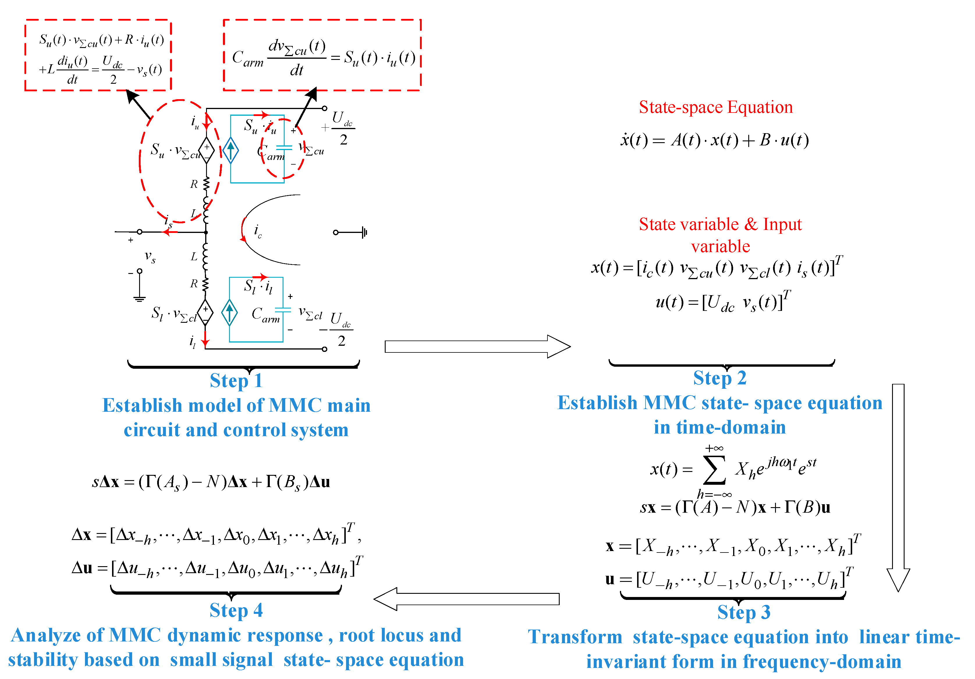
This paper follows the steps below, which are shown in Figure 1, in order to analyze the stability of MMC system. First, a model of MMC main circuit and control system are established; Second, the MMC state-space equation in time-domain is established. Next, the state-space equations are transformed into linear time-invariant form in frequency-domain. Finally, MMC dynamic response, root locus, and stability based on small signal state-space equation are analyzed.

When compared with the traditional state-space equation, the signal x(t) is expressed as an exponentially modulated periodic (EMP) signal to represent harmonic of different orders in the tome domain in Step 3 of Figure 1. On the other hand, because the MMC control system and electrical system are coupled with each other and control loops are coupled with each other, the Toeplitz matrix Γ(A) is applied to express the coupling of state variables with different frequencies in Step 3. Therefore, as compared with the traditional state-space model, the MMC small signal model that is based on harmonic state-space in this paper makes the analysis of dynamic characteristics, steady-state characteristics, and stability of MMC more accurate.

The rest of this paper is organized, as follows. Section 2 introduces the basic topology and operation theory of MMC and it derives the state-space equations in time domain. Section 3 builds the steady-state model and the small signal model of MMC based on the HSS method in open-loop control mode and dc-voltage control mode, respectively. Section 4 uses the eigenvalues and participation factors of the established HSS small signal model to analyze the stability of a dc-voltage controlled MMC system and the influence of controller parameters on the stability of the system. 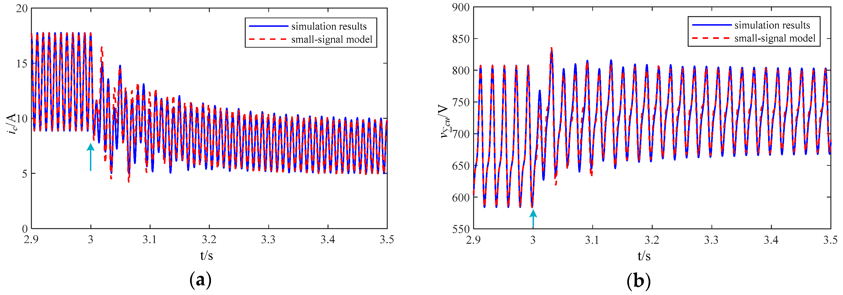Section 5 provides a case study of dc voltage-mode controlled MMC, and the simulation result verifies the validity of theoretical analyses. Section 6 concludes the work of this paper.

2. Basic Theory of MMC

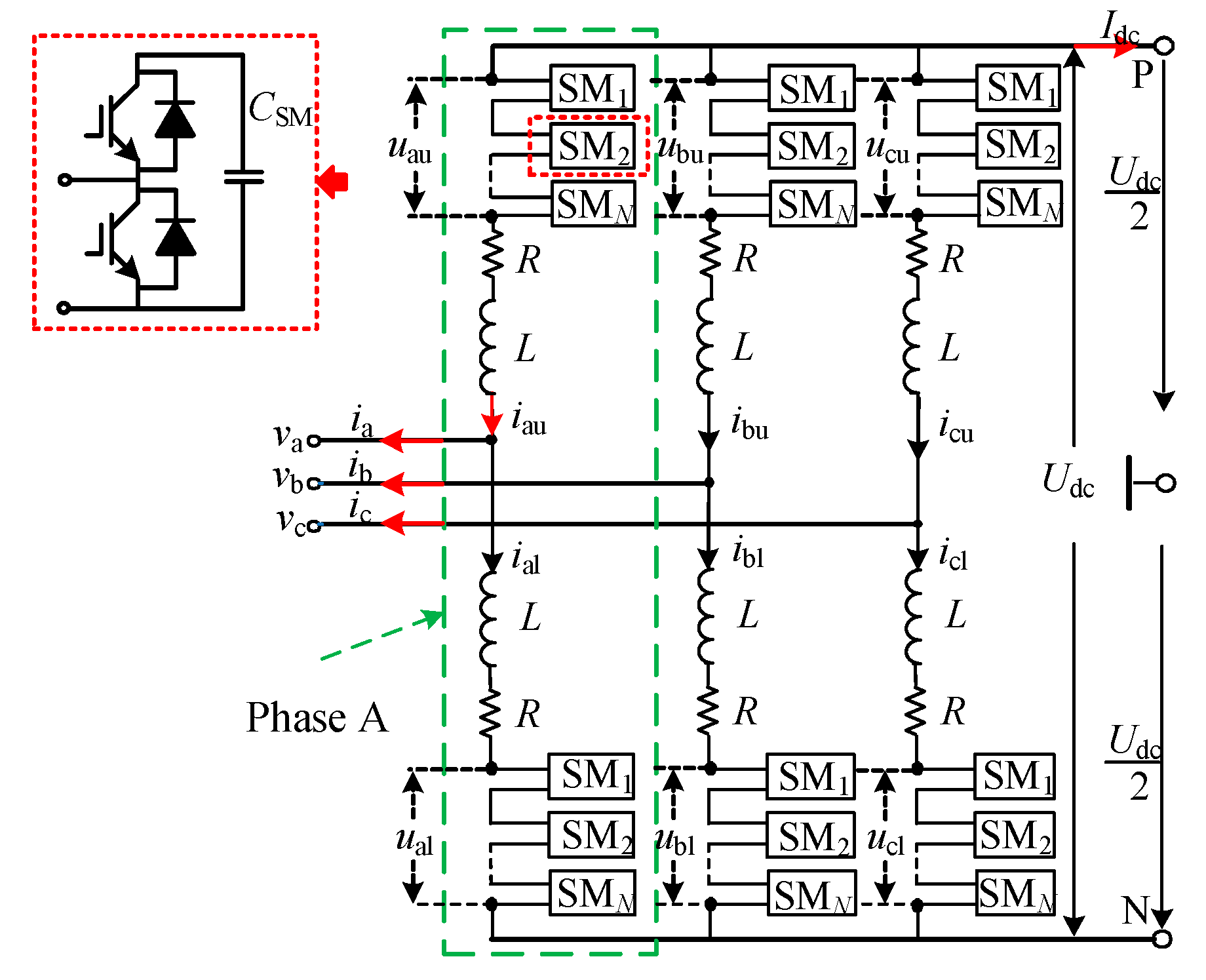
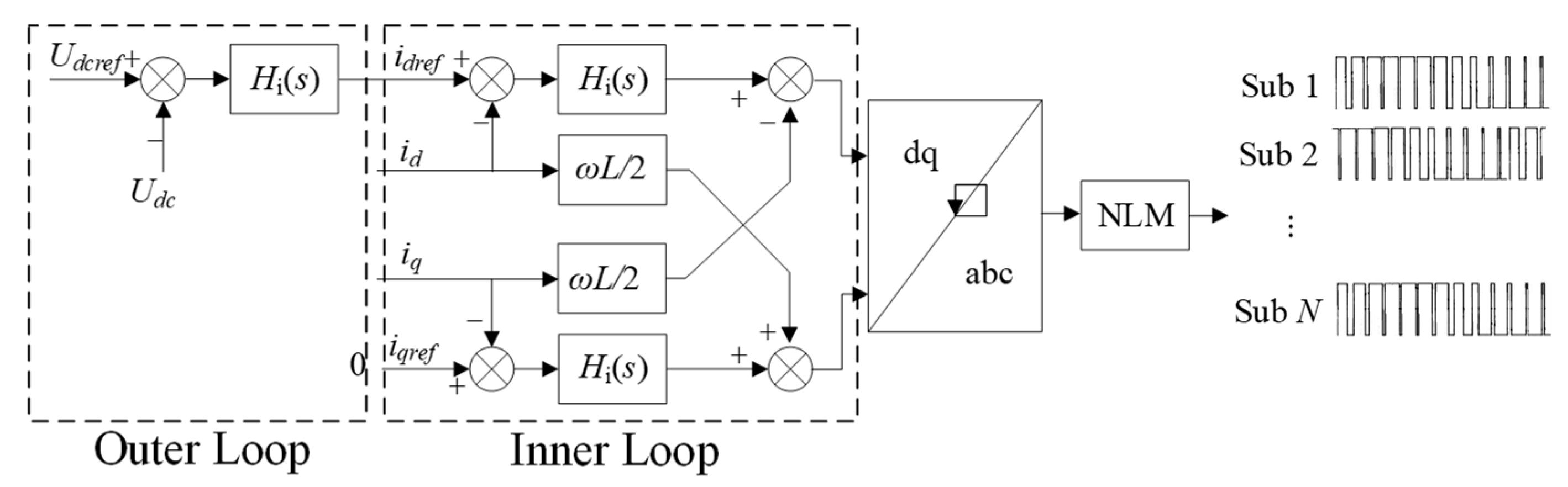
Figure 2 shows the basic structure of MMC. The converter consists of three phases, and each phase consists of one upper arm and one lower arm connected in series between two dc terminals. Each arm has N series-connected half-bridge submodules (SM) and one arm inductor L, the equivalent parasitic resistance of which is R. C_SM is capacitance of submodule capacitors, whose nominal voltages are all U_dc/N.

Figure 3 shows the control block diagram of MMC. The control system of MMC is divided into outer loop and inner loop, where outer loop is dc voltage control loop and inner loop is current control loop.

In outer control loop, the difference of dc voltage reference value and actual dc voltage value goes through a PI controller and generates current reference value in d axis. Inner control loop adopts the basic dq decoupling control strategy, as shown in Figure 3, where i_dref and i_qref are d-axis and q-axis current reference values, respectively. i_dref is given by the outer dc voltage control loop and i_qref is 0. The differences between the current reference values and actual current values go through PI controllers, dq inverse transformation, and nearest level approximation modulation (NLM) and modulation function in abc reference frame are finally generated.

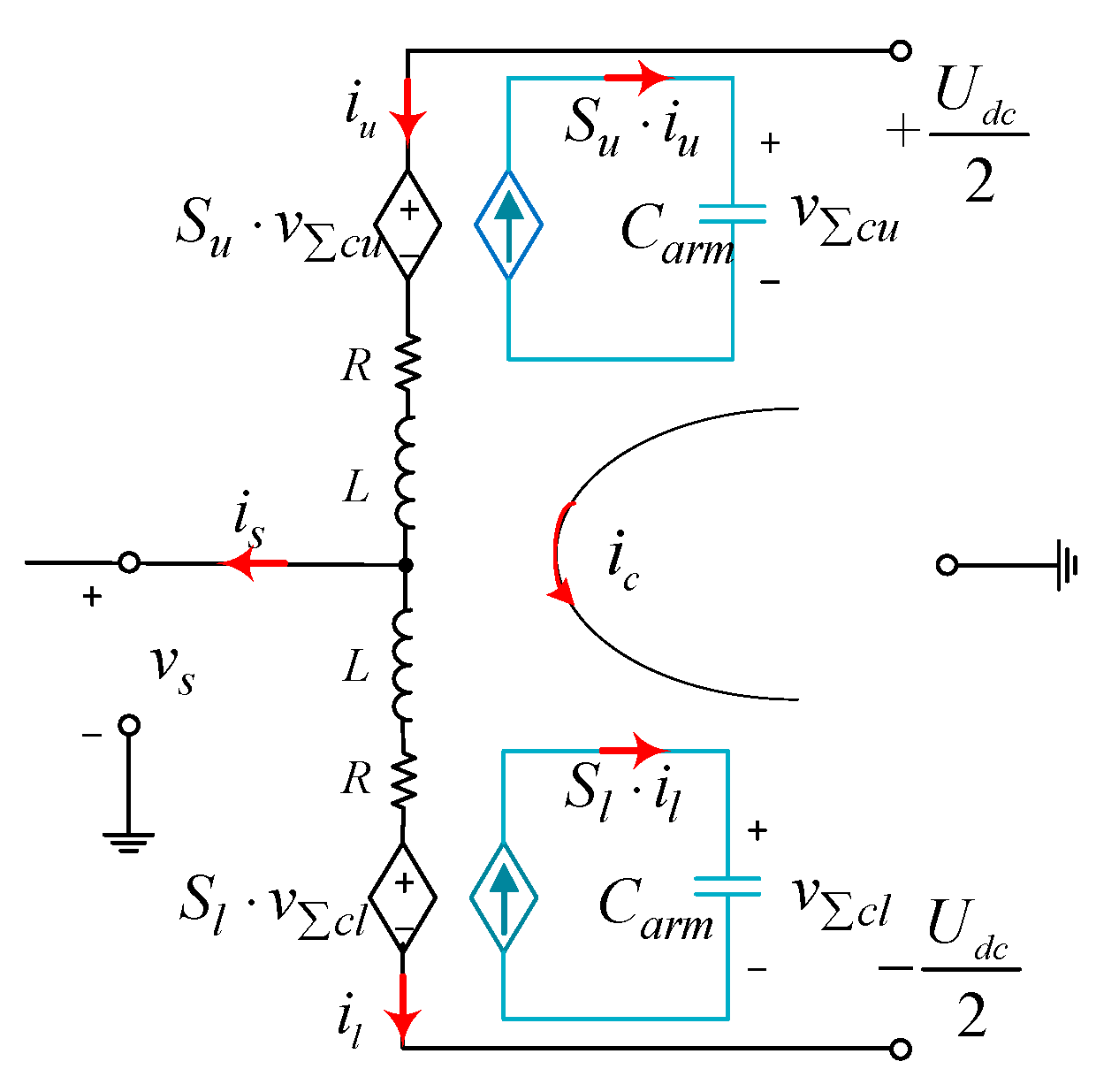
When the MMC operates in steady state, while assuming that capacitance voltages of all submodules are perfectly balanced, the average equivalent circuit of one phase could be constructed, as in Figure 4 [8]. Additionally, C_arm is the equivalent capacitance of one arm, where C_arm = C_SM/N. The switching functions of upper and lower arms are S_u and S_l respectively. v_s is the ac side phase voltage of the converter, and V_dc is the dc terminal voltage. v_∑cu and v_∑cl are the sum of the capacitor voltages of the upper and lower arms, respectively.

In Figure 4, the average switching functions of upper arm S_u and lower arm S_l are defined as:

$$S_u(t)=\frac{1-m(t)}{2}$$

(1)

$$S_l(t)=\frac{1+m(t)}{2}$$

(2)

where m(t) is the modulation function of this phase: m(t) = 2v_s(t)/U_dc.

While applying Kirchhoff’s law to this one-phase circuit of MMC, the equations of the upper and lower arms can be derived as:

$$S_u(t)\cdot v_{\sum cu}(t)+R\cdot i_u(t)+L\frac{d{i}_u(t)}{dt}=\frac{U_{dc}}{2}-v_s(t)$$

(3)

$$S_l(t)\cdot v_{\sum cl}(t)+L\frac{d{i}_l(t)}{dt}+R\cdot i_l(t)=\frac{U_{dc}}{2}+v_s(t)$$

(4)

The dynamic performance of the submodule capacitors can be obtained as:

$$C_{arm}\frac{d{v}_{\sum cu}(t)}{dt}=S_u(t)\cdot i_u(t)$$

(5)

$$C_{arm}\frac{d{v}_{\sum cl}(t)}{dt}=S_l(t)\cdot i_l(t)$$

(6)

The arm currents of upper and lower arms can be represented as:

$$i_u(t)=i_c(t)+\frac{i_s(t)}{2}$$

(7)

$$i_l(t)=i_c(t)-\frac{i_s(t)}{2}$$

(8)

where i_s is ac side phase current of the converter and i_c = (i_u + i_l)/2, which refers to the circulating current flowing through the upper and lower arms of the converter at the same time.

Note that the dc component of i_c is I_c0, and then the dc side current I_dc can be expressed as:

$$I_{dc}=-3I_{c0}$$

(9)

Substituting (7) and (8) into (3)–(6), the state-space equations of one-phase of MMC can be expressed as:

$$\dot{x}(t)=A(t)\cdot x(t)+B\cdot u(t)$$

(10)

where

$$\begin{array}{l}x(t)={[\begin{array}{cccc}{i}_c(t)& v_{\sum cu}(t)& v_{\sum cl}(t)& i_s\end{array}(t)]}^T\\ u(t)={[\begin{array}{cc}{U}_{dc}& v_s(t)\end{array}]}^T\end{array}$$

(11)

$$A(t)=\left[\begin{array}{cccc}-\frac{R}{L}& -\frac{(1-m(t))}{4L}& -\frac{(1+m(t))}{4L}& 0\\ \frac{(1-m(t))}{2C_{arm}}& 0& 0& \frac{(1-m(t))}{4C_{arm}}\\ \frac{(1+m(t))}{2C_{arm}}& 0& 0& -\frac{(1+m(t))}{4C_{arm}}\\ 0& -\frac{(1-m(t))}{2L}& \frac{(1+m(t))}{2L}& -\frac{R}{L}\end{array}\right]$$

(12)

$$B={\left[\begin{array}{cccc}\frac{1}{2L}& 0& 0& 0\\ 0& 0& 0& -\frac{2}{L}\end{array}\right]}^T$$

(13)

The above state-space equation of MMC indicates a nonlinear time periodic (NLTP) system. The detailed derivation process of converting this system into a linear time-invariant (LTI) system with the HSS method will be shown in the following section.

3. Small Signal Modeling of MMC Based on HSS

3.1. HSS-Based Large Signal Model of MMC Power Stage

Any time-varying periodic signal y(t) can be described as the form of Fourier series expansion:

$$y(t)={\displaystyle \sum _{h=-\infty }^{+\infty }{Y}_h{e}^{jh{\omega }_{1}t}}$$

(14)

where ω₁ = 2π/T₁ and T₁ is the fundamental period of the periodic signal, and h is the harmonic order.

Specially, the state variable x(t) is written as an exponentially modulated periodic (EMP) signal to represent the transient evolution of the harmonics:

$$x(t)={\displaystyle \sum _{h=-\infty }^{+\infty }{X}_h{e}^{jh{\omega }_{1}t}{e}^{st}}$$

(15)

where s = σ + jω is used to modulate the Fourier coefficient for extracting the transient response of harmonic components [18].

Based on the transformations (14) and (15), the NLTP state-space model in (10) of single phase of MMC in time-domain can be expressed as a LTI HSS model in the frequency-domain [19,20,21]:

$$sx=(\mathsf{\Gamma }(A)-N)x+\mathsf{\Gamma }(B)u$$

(16)

where

$$\begin{array}{l}x={[X_{-h},\cdots ,X_{-1},X_0,X_1,\cdots ,X_h]}^T\\ u={[U_{-h},\cdots ,U_{-1},U_0,U_1,\cdots ,U_h]}^T\end{array}$$

(17)

where X_n, U_n are, respectively, the nth Fourier coefficient of state variable x(t) and input variable u(t), and n = −h, … −1, 0, 1, …, h.

$$\begin{array}{l}{X}_n={[\begin{array}{cccc}{I}_{cn}& V_{\sum cun}& V_{\sum cln}& I_{sn}\end{array}]}^T\\ U_n={[\begin{array}{cc}{U}_{dcn}& V_{sn}\end{array}]}^T\end{array}$$

(18)

where I_cn is the nth Fourier coefficient of i_c(t), and V_∑cun is the nth Fourier coefficient of v_∑cuo(t). Other parameters have similar meanings, which are not explained repeatedly here.

Γ(A) and N in (16) are expressed as:

$$\mathsf{\Gamma }(A)=\left[\begin{array}{ccccccc}{A}_0& A_{-1}& \cdots & A_{-h}& & & \\ A_1& \ddots & \ddots & \ddots & \ddots & O& \\ ⋮& \ddots & A_0& A_{-1}& \ddots & \ddots & \\ A_h& \ddots & A_1& A_0& A_{-1}& \ddots & A_{-h}\\ & \ddots & \ddots & A_1& A_0& \ddots & ⋮\\ & O& \ddots & \ddots & \ddots & \ddots & A_{-1}\\ & & & A_h& \cdots & A_1& A_0\end{array}\right]$$

(19)

$$N=diag[-jh{\omega }_{1}I,\cdots ,0,\cdots ,jh{\omega }_{1}I]$$

(20)

Γ(A) is a Toeplitz matrix form of A, as shown in (19), which consists of the Fourier series of the matrix A, where A_n is the nth Fourier coefficient of A (n = −h, …, −1, 0, 1, …, h). O in (19) is zero matrix. I in (20) is the identity matrix, which has the same order as A.

When n = 0,

$$A_0=\left[\begin{array}{cccc}-\frac{R}{L}& -\frac{1}{4L}& -\frac{1}{4L}& 0\\ \frac{1}{2C_{arm}}& 0& 0& \frac{1}{4C_{arm}}\\ \frac{1}{2C_{arm}}& 0& 0& -\frac{1}{4C_{arm}}\\ 0& -\frac{1}{2L}& \frac{1}{2L}& -\frac{R}{L}\end{array}\right]$$

(21)

When n ≠ 0,

$$A_n=\left[\begin{array}{cccc}0& -\frac{(1-M_n)}{4L}& -\frac{(1+M_n)}{4L}& 0\\ \frac{(1-M_n)}{2C_{arm}}& 0& 0& \frac{(1-M_n)}{4C_{arm}}\\ \frac{(1+M_n)}{2C_{arm}}& 0& 0& -\frac{(1+M_n)}{4C_{arm}}\\ 0& -\frac{(1-M_n)}{2L}& \frac{(1+M_n)}{2L}& 0\end{array}\right]$$

(22)

Γ(B) in (16) is a Toeplitz matrix form of B, being similar to (19), which consists of the Fourier series of the matrix B, where B_n is the nth Fourier coefficient of B.

When n = 0,

$$B_n={\left[\begin{array}{cccc}\frac{1}{2L}& 0& 0& 0\\ 0& 0& 0& -\frac{2}{L}\end{array}\right]}^T$$

(23)

When n ≠ 0,

$$B_n={\left[\begin{array}{cccc}0& 0& 0& 0\\ 0& 0& 0& 0\end{array}\right]}^T$$

(24)

Equation (16) represents the steady-state model of single phase of MMC that is based on the HSS method, which is linearized from (10) and is a LTI system. Therefore, the stability of MMC can be analyzed with the classical control theory. This HSS model can not only obtain the information of the 0–hth harmonics, but also reflect the interactions between the harmonics.

Letting the left side of (16) to be zero, the steady-state solution of HSS model of MMC can be calculated by:

$$x={(-\mathsf{\Gamma }(A)+N)}^{-1}\mathsf{\Gamma }(B)u$$

(25)

where the frequency-domain values of state variables can be obtained. Referring to (14), the time-domain values of i_co(t), v_∑cuo(t), v_∑clo(t), and i_so(t) can be solved.

3.2. HSS-Based Small Signal Model of MMC with Open-loop Control

Based on Equations (3)–(6), the small-signal model of MMC around an operation trajectory (characterized by m_o(t), v_∑cuo(t), v_∑clo(t), i_so(t)) can be derived as:

$$\frac{d\Delta i_s(t)}{dt}=-\frac{(1-m_o(t))}{2L}\cdot \Delta v_{\sum cu}(t)+\frac{(1+m_o(t))}{2L}\cdot \Delta v_{\sum cl}(t)-\frac{R}{L}\cdot \Delta i_s(t)-\frac{2\Delta v_s}{L}+\frac{(v_{\sum cu}{}_o(t)+v_{\sum clo}(t))}{2L}\cdot \Delta m(t)$$

(26)

$$\frac{d\Delta i_c(t)}{dt}=-\frac{R}{L}\cdot \Delta i_c(t)-\frac{(1-m_o(t))}{4L}\cdot \Delta v_{\sum cu}(t)-\frac{(1+m_o(t))}{4L}\cdot \Delta v_{\sum cl}(t)+\frac{\Delta U_{dc}}{2L}+\frac{(v_{\sum cu}{}_o(t)-v_{\sum clo}(t))}{4L}\cdot \Delta m(t)$$

(27)

$$\frac{d\Delta v_{\sum cu}(t)}{dt}=\frac{(1-m_o(t))}{2C_{arm}}\cdot \Delta i_c(t)+\frac{(1-m_o(t))}{4C_{arm}}\cdot \Delta i_s(t)-\frac{(2i_{co}(t)+i_{so}(t))}{4C_{arm}}\cdot \Delta m(t)$$

(28)

$$\frac{d\Delta v_{\sum cl}(t)}{dt}=\frac{(1+m_o(t))}{2C_{arm}}\cdot \Delta i_c(t)-\frac{(1+m_o(t))}{4C_{arm}}\cdot \Delta i_s(t)+\frac{(2i_{co}(t)-i_{so}(t))}{4C_{arm}}\cdot \Delta m(t)$$

(29)

In open-loop control mode, the modulation signal m(t) is directly given, so it could serve as an input variable in the state-space model. While combining Equations (26)–(29), the small signal model of MMC in open-loop control mode, which is also the model of power stage of MMC, can be represented as:

$$\Delta \dot{x}(t)=A_s(t)\cdot \Delta x(t)+B_s(t)\cdot \Delta u(t)$$

(30)

where

$$\begin{array}{l}\Delta x={[\Delta \begin{array}{cccc}{i}_c(t)& \Delta v_{\sum cu}(t)& \Delta v_{\sum cl}(t)& \Delta i_s\end{array}(t)]}^T\\ \Delta u(t)={[\begin{array}{ccc}\Delta U_{dc}& \Delta v_s(t)& \Delta m(t)\end{array}]}^T\end{array}$$

(31)

$$A_s(t)=\left[\begin{array}{cccc}-\frac{R}{L}& -\frac{(1-m_o(t))}{4L}& -\frac{(1+m_o(t))}{4L}& 0\\ \frac{(1-m_o(t))}{2C_{arm}}& 0& 0& \frac{(1-m_o(t))}{4C_{arm}}\\ \frac{(1+m_o(t))}{2C_{arm}}& 0& 0& -\frac{(1+m_o(t))}{4C_{arm}}\\ 0& -\frac{(1-m_o(t))}{2L}& \frac{(1+m_o(t))}{2L}& -\frac{R}{L}\end{array}\right]$$

(32)

$$B_s(t)=\left[\begin{array}{ccc}\frac{1}{2L}& 0& \frac{v_{\sum cu}{}_o(t)-v_{\sum clo}(t)}{4L}\\ 0& 0& -\frac{2i_{co}(t)+i_{so}(t)}{4C_{arm}}\\ 0& 0& \frac{2i_{co}(t)-i_{so}(t)}{4C_{arm}}\\ 0& -\frac{2}{L}& \frac{v_{\sum cu}{}_o(t)+v_{\sum clo}(t)}{2L}\end{array}\right]$$

(33)

where i_co(t), v_∑cuo(t), v_∑clo(t), and i_so(t) represent the steady operation point of MMC, which can be solved from Equation (25).

By converting Equation (30) into a HSS equation, the small signal model of MMC with open-loop control mode can be expressed as:

$$s\Delta x=(\mathsf{\Gamma }(A_s)-N)\Delta x+\mathsf{\Gamma }(B_s)\Delta u$$

(34)

where

$$\begin{array}{l}\Delta x={[\Delta x_{-h},\cdots ,\Delta x_{-1},\Delta x_0,\Delta x_1,\cdots ,\Delta x_h]}^T\\ \Delta u={[\Delta u_{-h},\cdots ,\Delta u_{-1},\Delta u_0,\Delta u_1,\cdots ,\Delta u_h]}^T\end{array}$$

(35)

Γ(A_s) is the Toeplitz matrix form of A_s, and Γ(B_s) is the Toeplitz matrix form of B_s. The elements in (35), such as Δx_n, Δu_n, A_sn, and B_sn are the nth Fourier coefficients of Δx(t), Δu(t), A_s(t), B_s(t), and n = −h, …, −1, 0, 1, …, h.

3.3. HSS-Based Small Signal Model of MMC with DC-Voltage Control

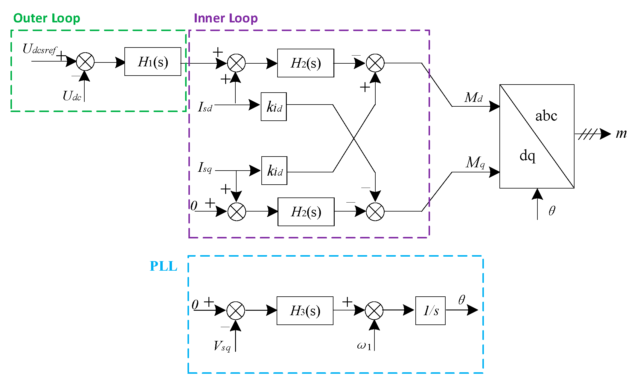
DC-voltage control is commonly used in an MMC-based HVDC system to maintain the dc bus voltage. Figure 5 shows the control structure, which contains outer dc-voltage control loop, inner current control loop, and phase-locked loop (PLL), where U_dc and U_dcref are the dc side voltage of MMC and its reference value, respectively. I_sd, I_sq are the values of MMC ac side current in dq coordinate system. V_sd, V_sq are the values of MMC ac side voltage in dq coordinate system, and M_d, M_q are the values of modulation signal in dq coordinate system. ω₁ is the fundamental angular frequency of 314.1 rad/s, and θ is the output phase angle of PLL. H₁(s), H₂(s), and H₃(s) are the PI controllers of dc voltage control, current control, and PLL control, respectively. k_id is the decoupling coefficient. The effect of small signal disturbance on PLL can be neglected when the converter is integrated with a strong enough ac grid [24]. Therefore, the small signal model of MMC in this paper does not take the effect of PLL into account.

3.3.1. Small Signal Model of Inner Current Control Loop

The inner current control loop contains two PI controller. Two additional state variables x_i1, x_i2 are introduced to simplify the integral operation:

$$\{\begin{array}{c}{x}_{i1}={\displaystyle \int I_{sd}dt}\Rightarrow \frac{d{x}_{i1}}{dt}=I_{sd}\\ x_{i2}={\displaystyle \int I_{sq}dt}\Rightarrow \frac{d{x}_{i2}}{dt}=I_{sq}\end{array}$$

(36)

where k_p2 and k_i2 are proportional coefficients and integral coefficients of the PI controllers in current control loop respectively.

Then the output small signal insertion indexes ΔM_d1, ΔM_q1 in dq coordinate system of the inner loop are:

$$\{\begin{array}{c}\Delta M_{d1}=-(k_{p2}\cdot \Delta I_{sd}+k_{i2}\cdot \Delta x_{i1})+k_{id}\cdot \Delta I_{sq}\\ \Delta M_{q1}=-(k_{p2}\cdot \Delta I_{sq}+k_{i2}\cdot \Delta x_{i2})-k_{id}\cdot \Delta I_{sd}\end{array}$$

(37)

The ΔM_d1, ΔM_q1 in dq coordinate system need to be transformed into Δm_i(t) in abc coordinate system, where Δm_i(t) is the control signal of phase A that is produced by the inner loop. Firstly, according to the dq transformation matrix, I_sd and I_sq can be expressed as:

$$\left[\begin{array}{l}{I}_{sq}\\ I_{sd}\\ I_{s0}\end{array}\right]=T_{dq}\cdot \left[\begin{array}{c}I\cos ({\omega }_{1}t+\phi )\\ I\cos ({\omega }_{1}t-\frac{2\pi }{3}+\phi )\\ I\cos ({\omega }_{1}t+\frac{2\pi }{3}+\phi )\end{array}\right]=\left[\begin{array}{c}-I\sin \phi \\ I\cos \phi \\ 0\end{array}\right]$$

(38)

where the Park transformation matrix T_dq is:

$$T_{dq}=\frac{2}{3}\left[\begin{array}{ccc}\sin ({\omega }_{1}t)& \sin ({\omega }_{1}t-\frac{2\pi }{3})& \sin ({\omega }_{1}t+\frac{2\pi }{3})\\ \cos ({\omega }_{1}t)& \cos ({\omega }_{1}t-\frac{2\pi }{3})& \cos ({\omega }_{1}t+\frac{2\pi }{3})\\ \frac{1}{2}& \frac{1}{2}& \frac{1}{2}\end{array}\right]$$

(39)

From Equation (38), the relationships between I_sd, I_sq, the amplitude I, and the phase angle φ of phase A current are:

$$\{\begin{array}{c}{I}_{sd}=-I\sin \phi \\ I_{sq}=I\cos \phi \end{array}$$

(40)

Combining Equations (14), (36) and (40), Equation (36) in time-domain can be represented in the frequency-domain:

$$\{\begin{array}{l}s{x}_{i1}=j{I}_{s+1}-j{I}_{s-1}\\ s{x}_{i2}=I_{s+1}+I_{s-1}\end{array}$$

(41)

According to inverse Park transformation matrix, Δm_i(t) could be calculated as:

$$T_{d{q}^{-1}}\cdot \left[\begin{array}{c}\Delta M_{d1}\\ \Delta M_{q1}\\ 0\end{array}\right]=\left[\begin{array}{c}\Delta M_{d1}\sin ({\omega }_{1}t)+\Delta M_{q1}\cos ({\omega }_{1}t)\\ -\Delta M_{d1}\cos ({\omega }_{1}t-\frac{\pi }{6})+\Delta M_{q1}\sin ({\omega }_{1}t-\frac{\pi }{6})\\ \Delta M_{d1}\cos ({\omega }_{1}t+\frac{\pi }{6})-\Delta M_{q1}\sin ({\omega }_{1}t+\frac{\pi }{6})\end{array}\right]$$

(42)

where the inverse Park transformation matrix T_dq⁻¹ is:

$$T_{d{q}^{-1}}=\left[\begin{array}{ccc}\sin ({\omega }_{1}t)& \cos ({\omega }_{1}t)& 1\\ \sin ({\omega }_{1}t-\frac{2\pi }{3})& \cos ({\omega }_{1}t-\frac{2\pi }{3})& 1\\ \sin ({\omega }_{1}t+\frac{2\pi }{3})& \cos ({\omega }_{1}t+\frac{2\pi }{3})& 1\end{array}\right]$$

(43)

According to the complex form of Fourier expansion, the ±1st coefficients of Δm_i(t) are:

$$\{\begin{array}{c}\Delta m_{i+1}=-\frac{j}{2}\cdot \Delta M_{d1}+\frac{1}{2}\cdot \Delta M_{q1}\\ \Delta m_{i-1}=\frac{j}{2}\cdot \Delta M_{d1}+\frac{1}{2}\cdot \Delta M_{q1}\end{array}$$

(44)

Substituting (37) and (41) into (44) the ±1st coefficients of Δm_i(t) are:

$$\{\begin{array}{c}\Delta m_{i+1}=\underset{1}{\underbrace{-(k_{p2}+j{k}_{id})\Delta I_{s+1}}}+\underset{2}{\underbrace{\frac{j}{2}{k}_{i2}\Delta x_{i1}}}\underset{3}{\underbrace{-\frac{1}{2}{k}_{i2}\Delta x_{i2}}}\\ \Delta m_{i-1}=\underset{1}{\underbrace{-(k_{p2}-j{k}_{id})\Delta I_{s-1}}}\underset{2}{\underbrace{-\frac{j}{2}{k}_{i2}\Delta x_{i1}}}\underset{3}{\underbrace{-\frac{1}{2}{k}_{i2}\Delta x_{i2}}}\end{array}$$

(45)

3.3.2. Small Signal Model of Outer DC-Voltage Control Loop

As shown in Figure 5, the difference between the actual value of the dc voltage and the reference value would pass through the outer loop PI controller and then the inner loop PI controller, producing small signal insertion index ΔM_d2 in d axis. Two additional state variables x_v1, x_v2 are introduced to achieve the integral operation of dc components for two integral components:

$$\{\begin{array}{l}{x}_{v1}={\displaystyle \int (U_{dcref}-U_{dc})dt\Rightarrow \frac{d{x}_{v1}}{dt}=U_{dcref}-U_{dc}}\\ x_{v2}={\displaystyle \int [k_{p1}(U_{dcref}-U_{dc})+k_{i1}\cdot x_{v1}]dt}\Rightarrow \frac{d{x}_{v2}}{dt}=k_{p1}(U_{dcref}-U_{dc})+k_{i1}{x}_{v1}\end{array}$$

(46)

where k_p1 and k_i1 are the proportional and integral coefficients of the PI controllers in outer DC voltage control loop, respectively. Afterwards, the output control signal ΔM_d2 is:

$$\Delta M_{d2}=-k_{p2}\cdot [k_{p1}(\Delta U_{dcref}-\Delta U_{dc})+k_{i1}\Delta x_{v1}]-k_{i2}\Delta x_{v2}$$

(47)

According to inverse Park transformation matrix, the control signal Δm_v(t) of phase A in abc coordinate system can be obtained from

$$T_{d{q}^{-1}}\cdot \left[\begin{array}{c}\Delta M_{d2}\\ 0\\ 0\end{array}\right]=\left[\begin{array}{c}\Delta M_{d2}\sin ({\omega }_{1}t)\\ -\Delta M_{d2}\cos ({\omega }_{1}t-\frac{\pi }{6})\\ \Delta M_{d2}\cos ({\omega }_{1}t+\frac{\pi }{6})\end{array}\right]$$

(48)

According to the complex form of Fourier expansion, the ±1st coefficients of Δm_v(t) are:

$$\{\begin{array}{c}\Delta m_{v+1}=-\frac{j}{2}\cdot \Delta M_{d2}\\ \Delta m_{v-1}=\frac{j}{2}\cdot \Delta M_{d2}\end{array}$$

(49)

Assume the equivalent impedance on the dc side is Z_L. According to Equation (9), ΔU_dc is

$$\Delta U_{dc}=\Delta I_{dc}{Z}_L=-3\Delta I_{c0}{Z}_L$$

(50)

Substituting (47) and (50) into (49), the ±1st coefficients of Δm_v(t) can be represented, as follows:

$$\{\begin{array}{c}\Delta m_{v+1}=\underset{1}{\underbrace{\frac{j}{2}{k}_{p2}{k}_{p1}\Delta U_{dcref}}}+\underset{2}{\underbrace{\frac{3j}{2}{k}_{p2}{k}_{p1}{Z}_L\Delta I_{c0}}}+\underset{3}{\underbrace{\frac{j}{2}{k}_{p2}{k}_{i1}\Delta x_{v1}}}+\underset{4}{\underbrace{\frac{j}{2}{k}_{i2}\Delta x_{v2}}}\\ \Delta m_{v-1}=\underset{1}{\underbrace{-\frac{j}{2}{k}_{p2}{k}_{p1}\Delta U_{dcref}}}\underset{2}{\underbrace{-\frac{3j}{2}{k}_{p2}{k}_{p1}{Z}_L\Delta I_{c0}}}\underset{3}{\underbrace{-\frac{j}{2}{k}_{p2}{k}_{i1}\Delta x_{v1}}}\underset{4}{\underbrace{-\frac{j}{2}{k}_{i2}\Delta x_{v2}}}\end{array}$$

(51)

3.3.3. Small Signal Model of DC-Voltage Controlled MMC

The models of control system and open-loop system need to be integrated into one state-space equation in order to establish the small signal model of the entire closed-loop system of MMC.

The state variables of the closed-loop system of MMC include four state variables of power stage (Δi_c, Δv_∑cu, Δv_∑cl, Δi_s) and four state variables of control system (Δx_i1, Δx_i2, Δx_v1, Δx_v2):

$$\Delta x(t)={\left[\begin{array}{cccccccc}\Delta i_c(t)& \Delta v_{\sum cu}(t)& \Delta v_{\sum cl}(t)& \Delta i_s(t)& \Delta x_{i1}& \Delta x_{i2}& \Delta x_{v1}& \Delta x_{v2}\end{array}\right]}^T$$

(52)

The input variables of the closed-loop system of MMC are the same as the input variables of the power stage of MMC:

$$\Delta u_c(t)={[\begin{array}{cc}\Delta U_{dcref}& \Delta v_s(t)\end{array}]}^T$$

(53)

By combining the equations of control system (36), (45), (46) and (51) with the HSS model of power stage in (34), the HSS model of the entire closed-loop system can be expressed as:

$$s\Delta x=(A_c-N)\Delta x+B_c\Delta u_c$$

(54)

where:

$$\begin{array}{l}\Delta x={[\Delta x_{-h},\cdots ,\Delta x_{-1},\Delta x_0,\Delta x_{+1},\cdots ,\Delta x_{+h}]}^T\\ \Delta u={[\Delta u_{-h},\cdots ,\Delta u_{-1},\Delta u_0,\Delta u_{+1},\cdots ,\Delta u_{+h}]}^T\end{array}$$

(55)

$$A_c=\left[\begin{array}{ccccccccc}{A}_0& A_{-1}& A_{-2}& \cdots & A_{-h}& & & & \\ A_{+1}& \ddots & \ddots & \ddots & \ddots & \ddots & & O& \\ A_{+2}& \ddots & A_0& A_{-1}& A_{-2}& \ddots & \ddots & & \\ ⋮& \ddots & A_{+1}& A_{0N}& A_{-1O}& A_{-2}& \ddots & \ddots & \\ A_{+h}& \ddots & A_{+2}& A_{+1N}& A_{0O}& A_{-1P}& A_{-2}& \ddots & A_{-h}\\ & \ddots & \ddots & A_{+2}& A_{+1O}& A_{0P}& A_{-1}& \ddots & ⋮\\ & & \ddots & \ddots & A_{+2}& A_{+1}& A_0& \ddots & A_{-2}\\ & O& & \ddots & \ddots & \ddots & \ddots & \ddots & A_{-1}\\ & & & & A_{+h}& \cdots & A_{+2}& A_{+1}& A_0\end{array}\right]$$

(56)

$$B_c=\left[\begin{array}{ccccccccc}{B}_0& B_{-1}& B_{-2}& \cdots & B_{-h}& & & & \\ B_{+1}& \ddots & \ddots & \ddots & \ddots & \ddots & & O& \\ B_{+2}& \ddots & B_0& B_{-1}& B_{-2}& \ddots & \ddots & & \\ ⋮& \ddots & B_{+1}& B_0& B_{-1O}& B_{-2}& \ddots & \ddots & \\ B_{+h}& \ddots & B_{+2}& B_{+1}& B_{0O}& B_{-1}& B_{-2}& \ddots & B_{-h}\\ & \ddots & \ddots & B_{+2}& B_{+1O}& B_0& B_{-1}& \ddots & ⋮\\ & & \ddots & \ddots & B_{+2}& B_{+1}& B_0& \ddots & B_{-2}\\ & O& & \ddots & \ddots & \ddots & \ddots & \ddots & B_{-1}\\ & & & & B_{+h}& \cdots & B_{+2}& B_{+1}& B_0\end{array}\right]$$

(57)

Additionally, N is the same as (20).

The variables Δx_i1, Δx_i2, Δx_v1, Δx_v2, and ΔU_dcref in (55) are all dc components. When these variables are transformed into Fourier series, they only have values at the frequency of 0 Hz, and the components of other frequencies are zero.

The control signals Δm_i+1, Δm_i−1, Δm_v+1, and Δm_v−1 in (56) are added to the system matrix A_c, and they are only related to the matrix components A_0O, A_0P, A_0N, A_−1O, A_−1N, A_1O, and A_1P. The other matrix components A₀, A₊₁, A₋₁, A₊₂, A₋₂ … are only dependent on the main circuit of MMC. Subsequently, the specific expressions of these matrix are presented in the Appendix A.

Similarly, for the input matrix B_c, as shown in (57), the controlling signals Δm_v+1 and Δm_v−1 need to be added into the matrix, and they are only related to the matrix components B_0O, B_+1O, and B_−1O. The specific expressions are also presented in the Appendix A.

In general case, circulating current mainly contains dc and second harmonic components and the capacitor voltages mainly contains dc, fundamental, second and third harmonic components. Therefore, the harmonic order considered in the HSS model is h = 3.

4. Stability Analysis Based on the HSS-Based Small Signal Model

Table 1. The main parameters of MMC in calculation and simulation.

Parameter	Value
DC side voltage Udc/V	700
AC side voltage vs/V	310
Number of SMs on one arm	20
Arm inductance L/mH	15
Arm resistance R/mΩ	0.1
SM capacitor CSM /μF	7200

shows the main parameters of the studied MMC. It is worth mentioning that the number of modules in one arm is 20 to reduce the simulation time. Figure 5 shows the MMC operates in dc voltage control mode. Firstly, the outer loop controller parameters are set as k_p1 = 0.87 and k_i1 = 10, the inner loop controller parameters are set as k_p2 = 0.019 and k_i2 = 0.057. It needs to be noted that, since the four state variables of control system Δx_i1, Δx_i2, Δx_v1, and Δx_v2 only have values at the frequency of 0 Hz, they do not have significance at other frequencies (−3ω₁, −2ω₁, −1ω₁, 1ω₁, 2ω₁, 3ω₁). Thus, there are always 24 eigenvalues at the origin (0, j0), having no effect on the stability analysis of the system. After calculation, it is confirmed that in addition to these 24 eigenvalues, there is another eigenvalue that is located at the origin. Therefore, these 25 eigenvalues will not be discussed in this paper. Additionally, other eigenvalues are plotted as shown in Figure 6. It can be seen that all eigenvalues are on the left half plane of the complex plane, which indicated that the MMC system is stable with these controller parameters.

The concept of oscillation mode is introduced, that is, a real root or a pair of conjugate complex roots represent one oscillation mode of the system in order to further analyze the eigenvalues. Additionally, the participation factor analysis is introduced to analyze the interaction between state variables and oscillation modes. The participation factor of the kth state variable in the ith oscillation mode of the system can be calculated by [25]:

$$P_{ki}={\Phi }_{ki}{\Psi }_{ik}$$

(58)

where Φ_ki is the element in the kth row and ith column of the right eigenvector matrix, and Ψ_ik is the element in the ith row and kth column of the left eigenvector matrix.

Table 2. The oscillation modes of the MMC systems and their main participating state variables.

Oscillation Mode	Eigenvalue	Oscillation Frequency (Hz)	Participating State Variable
1	λ1,2 = −141.617724 ± 427.494287i	68.037	Δic0
2	λ3,4 = −0.003333 ± 529.349354i	84.248	Δic1
3	λ5,6 = −0.003333 ± 99.017871i	15.759	Δic1
4	λ7,8 = −13.492959 ± 413.017170i	65.733	Δic2
5	λ9,10 = −15.070545 ± 827.734452i	131.738	Δic2
6	λ11,12 = −0.003333 ± 757.351868i	120.536	Δic3
7	λ13,14 = −0.003333 ± 1187.683351i	189.025	Δic3
8	λ15,16 = −0.003333 ± 215.165741i	34.244	Δis0
9	λ17,18 = −777.873222 ± 564.833532i	89.896	Δis1
10	λ19,20 = −0.003333 ± 414.542740i	65.976	Δis2
11	λ21,22 = −0.003333 ± 844.874223i	134.465	Δis2
12	λ23.24 = −0.157052 ± 756.783394i	120.445	Δis3
13	λ25,26 = −0.628342 ± 1187.336919i	188.970	Δis3
14	λ27,28 = −13.608391 ± 176.910594i	27.691	Δucu0, Δucu1, Δucl0, Δucl1
15	λ29,30 = −3.728758 ± 2.717311i	0.432	Δxv11
16	λ31 = −2.47713152442756	0	Δxv21

Δi_cn, Δi_sn, Δu_cun, Δu_cln, Δx_v1n, Δx_v2n is nth harmonic component of Δi_c(t), Δi_s(t), Δu_cu(t), Δu_cl(t), Δx_v1(t), Δx_v2(t), respectively, and n = 0, 1, 2, 3.

lists the oscillation modes of the MMC systems and their main participating state variables, according to the value of the participation factors.

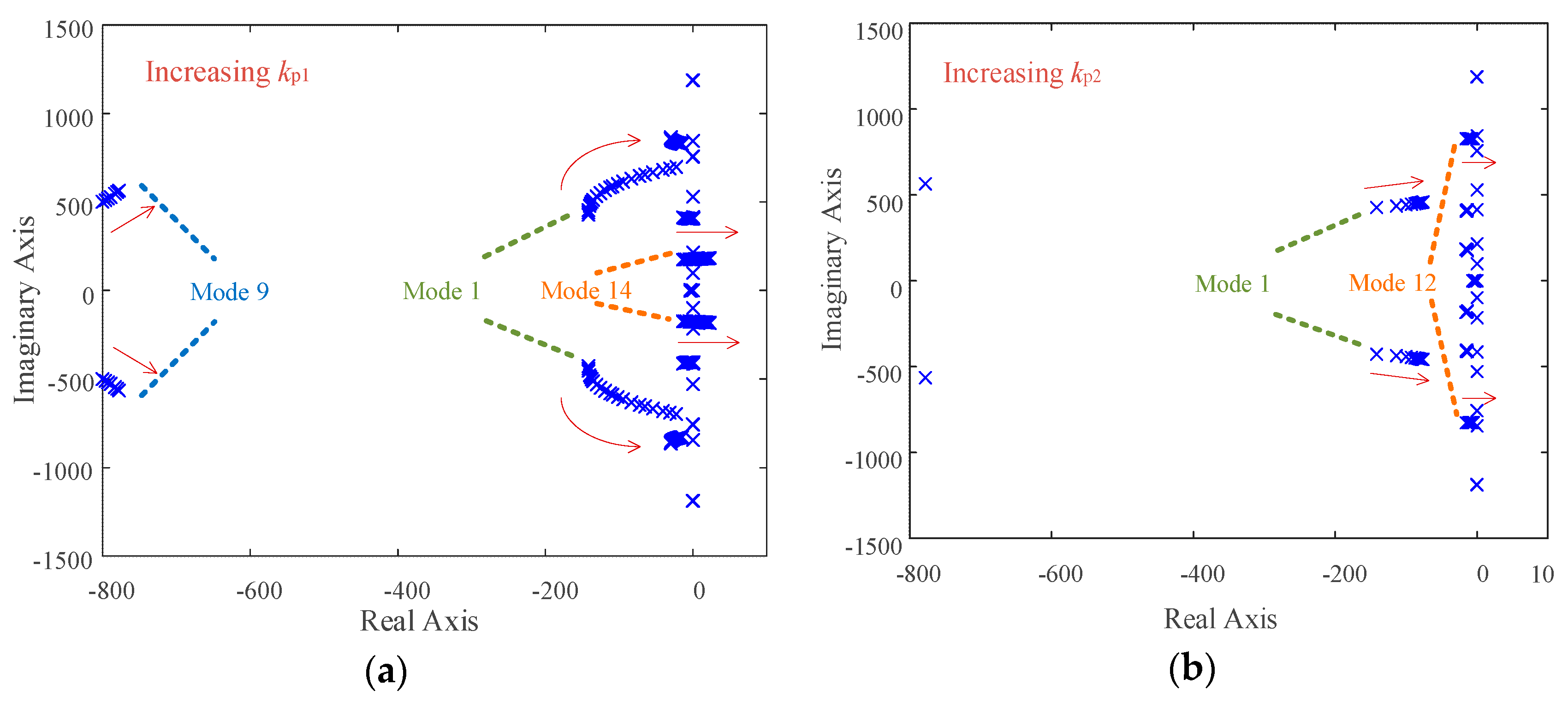
Eigenvalue loci when k_p1 and k_p2 changes are shown in Figure 7a,b, respectively, to analyze the effect of the controller parameters on the stability of MMC. When increasing the parameter k_p1 of outer voltage loop with other parameters unchanged, as shown in Figure 7a, oscillation modes 2, 3, 6, 7, 8, 10, 11 remain unchanged, which means that these eigenvalues are not affected by the change of k_p1 and most of other oscillation modes move to the right. As k_p1 gradually increases, oscillation modes 4, 12, 14, 15 move horizontally to the right whose imaginary parts are nearly unchanged. 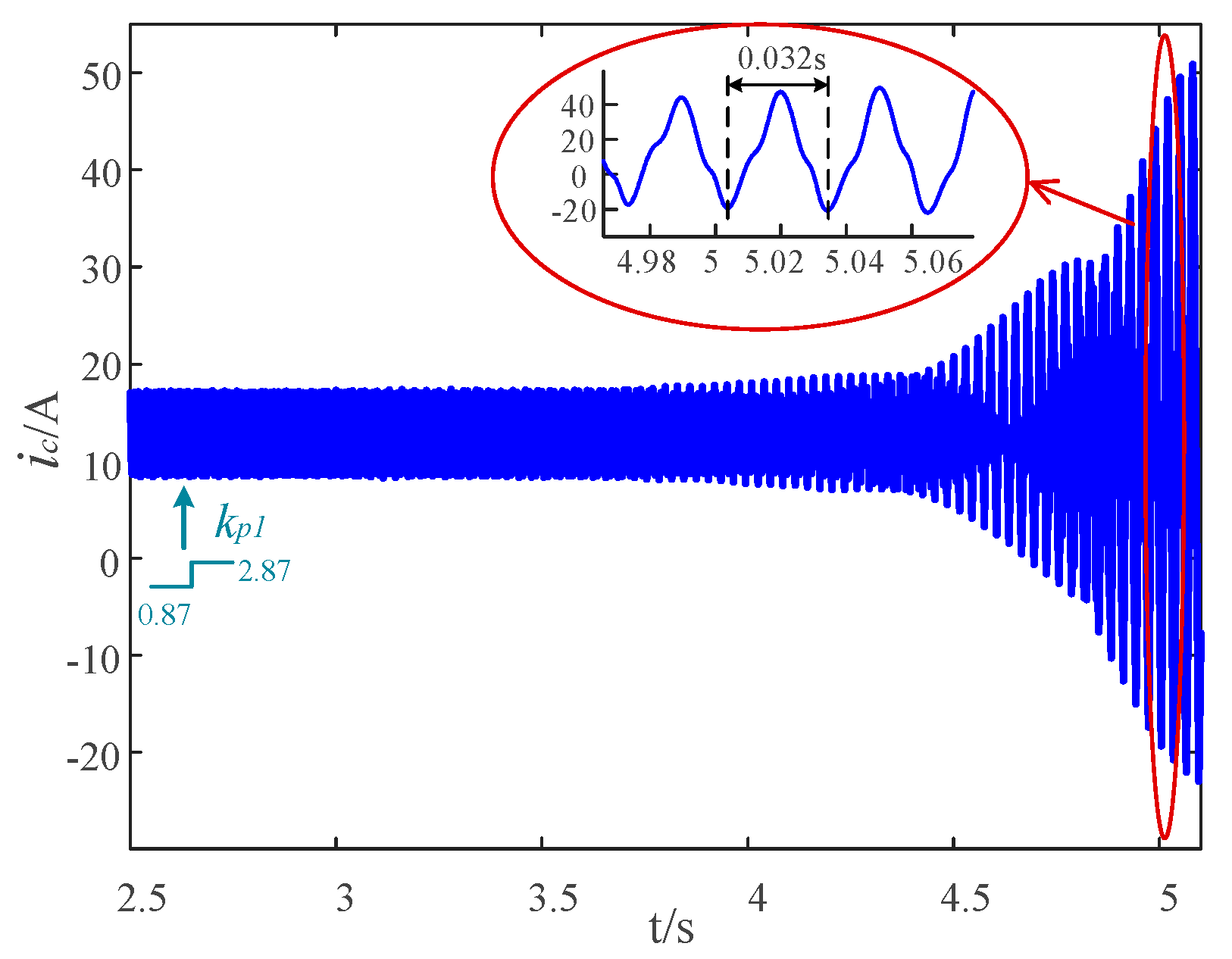Additionally, when k_p1 is 1.57, oscillation mode 14 firstly moves to the right half plane, which causes the instability of the system. For example, when k_p1 = 2.87, the eigenvalues of oscillation mode 14 are (4.196 ± j176.9). The corresponding oscillation period is 2π/176.9 = 0.0355 s.

Based on the analysis of participation factor, the oscillation mode 14 is strongly related to the dc component of the submodule capacitor voltage. It indicates that the instability is due to the change of proportional coefficient k_p1 of the outer dc voltage controller, which affects the dc component of submodule capacitor voltage, in turn causing oscillation mode 14 to move to the right half plane and causes instability.

Only the eigenvalues whose imaginary parts remain unchanged could cross into the right half plane, even if k_p1 continues to increase. This indicates that with the dc-voltage control mode, the change of controller parameter k_p1 will not change the unstable oscillation frequency of the MMC system.

When increasing the proportional coefficient k_p2 of inner current control loop with other parameters unchanged, as shown in Figure 7b, oscillation modes 2, 3, 6, 7, 8, 10, 11 remain unchanged, which means that these eigenvalues will not be affected by the change of k_p2, and most of other oscillation modes move to the right. As k_p2 gradually increases, oscillation modes 5, 12, 13, and 15 move horizontally to the right, whose imaginary parts are nearly unchanged. 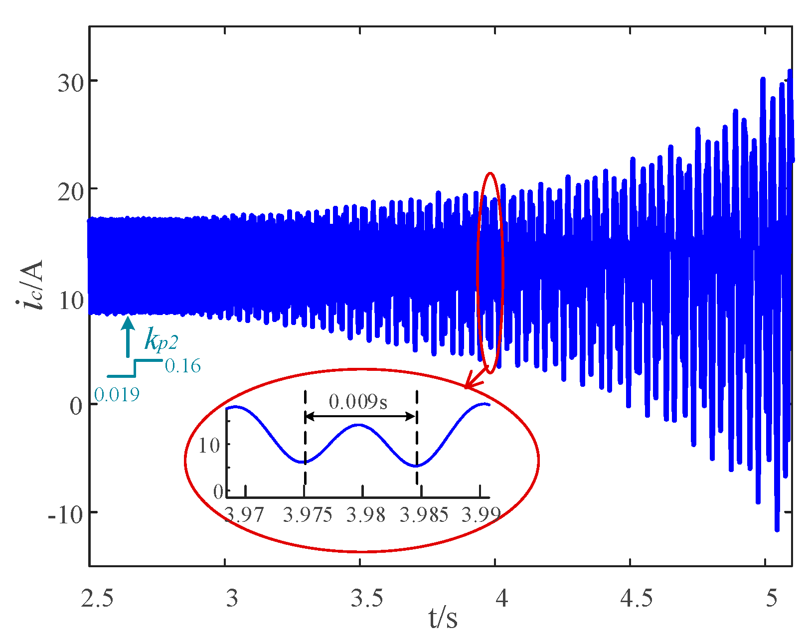Additionally, when k_p2 is 0.042, oscillation mode 12 firstly moves to the right half plane, which causes the instability of the system. For example, when k_p2 = 0.16, eigenvalues of oscillation mode 12 are (0.107 ± j756.8). The corresponding oscillation period is 2π/756.8 = 0.0083 s.

The oscillating modes 12 is related to the third frequency component of the ac side current based on the analysis of participation factors. It indicates that the instability is due to the change of proportional coefficient k_p2 of inner current controller, which affects the third frequency component of the ac side current, in turn causing the oscillation mode 12 to move to the right half plane and cause instability.

Even if k_p2 continues to increase, only the eigenvalues whose imaginary parts remain unchanged could cross into the right half plane, which indicated that with the dc-voltage control mode, the change of controller parameter k_p2 will also not change the unstable oscillation frequency of the MMC system.

5. Simulation Verifications

The small signal model of MMC that is based on HSS method is built in m. file in MATLAB and the considered order is set to be 3 in the model. Time-domain simulations are carried out in the MTLAB/Simulink and parameters adopted are as shown in Table 1 to validate the theoretical analysis.

5.1. Open-Loop Control Mode

When MMC operates in open-loop control mode and the reference of m(t) has a step change from 0.885sin(ω₁t + φ) to 0.87sin(ω₁t + φ) at 3 s, the transient response of i_c(t) is presented in Figure 8a and the zoom-in view is shown in Figure 8b, showing good agreement between the small-signal model and the simulation results.

Figure 9 shows the harmonic components of Δi_c(t) with open-loop control mode, which indicated that fundamental component’s change of m(t) would result in both dc and second harmonic components’ changes of i_c(t), which proves that the small-signal model that is presented in this paper could reflect the internal harmonic interactions of MMC.

5.2. DC-Voltage Control Mode

When MMC operates in dc-voltage control mode and the dc voltage reference value U_dcref has a step change from 700 V to 735 V at 3 s, the transient response of i_c(t) is presented in Figure 10a, and the transient response of v_∑cu(t) is presented in Figure 10b, all showing good agreement between the small-signal model and simulation results, thus verifying the accuracy of the modeling presented in this paper.

The outer loop controller parameter k_p1 is first changed to 2.87 o verify the predicted oscillation period with different parameters, while other parameters remain unchanged in the simulation model. Figure 11 shows the simulation waveform of i_c(t) with k_p1 = 2.87. It can be seen that the MMC system is unstable and the measured oscillation period of i_c(t) is approximately 0.032 s, which is almost consistent with the predicted oscillation period 2π/176.9 = 0.0355 s in Section 4.

Subsequently, the inner loop controller parameter k_p2 is changed to 0.162, while other parameters in the simulation model remain unchanged. Figure 12 shows the simulation waveform of i_c(t) with k_p2 = 0.162. It can be seen that the MMC system is unstable, and the measured oscillation period of i_c(t) is about 0.009 s, which is almost consistent with the predicted oscillation period 2π/756.8 = 0.0083 s in Section 4.

6. Conclusions

An accurate and complete small signal model of MMC with dc voltage control mode that is based on the HSS modeling method is derived, which considers the internal and external harmonic interactions, thus achieving higher accuracy. Subsequently, through the analysis of the eigenvalues, participation factors, and the calculation of oscillation frequencies under different controller parameters, the effect of controller parameters on the stability of MMC is studied and the following conclusions can be drawn. Besides, the time-domain simulation built in MATLAB/Simulink verifies the accuracy of the HSS-based MMC model and validity of stability analysis.

(1)

When MMC operates with dc-voltage control mode, either too large outer loop proportional coefficient k_p1 or inner loop proportional coefficient k_p2 might cause the system unstable.

(2)

The too large proportional coefficient k_p1 of outer dc voltage control loop will cause an oscillation mode with certain frequency, while the too large proportional coefficient k_p2 of inner current control loop will cause another oscillation mode with another certain frequency.