Impact of Phase Locked Loop with Different Types and Control Dynamics on Resonance of DFIG System

Abstract

In recent years, the doubly fed induction generator (DFIG) operates in a weak grid, rather than a strong grid due to the high proportion of wind energy into the power grid. The impedance interaction between the DFIG system and series and parallel compensated weak grid might cause the subsynchronous resonance (SSR) and high frequency resonance (HFR) in the DFIG system, respectively. Phase locked loop (PLL) is a popular grid synchronization technique, and the high bandwidth PLL can cause resonance at middle frequencies in the DFIG system. However, the impact of PLL types and their controller dynamics on the resonance in the DFIG system are not adequately researched. The impact of the PLL controller with different types, such as synchronous reference frame (SRF) and Lead/Lag PLL, is studied in this paper to fill this gap. Additionally, an improved PLL is proposed, which can guarantee the high phase margin and decrease the likelihood of the resonance at middle frequencies in the DFIG system under a weak grid. Moreover, the phase margin of the DFIG system impedance with an improved PLL is less sensitive to its controller parameters. Simulation and experimental results verify the effectiveness of the proposed method.

1. Introduction

The cost-effective variable speed operations and partial size power converter make the doubly fed induction generator (DFIG) prevalent in a modern wind power plant [1]. In recent years, the increasing growth of the DFIG system into a weak power system with large impedance might be seen [2,3,4], where the stable and secure operation of the DFIG system is contestable.

The subsynchronous resonance (SSR) [5,6,7,8,9,10,11] and high frequency (HFR) [12,13,14,15,16] may occur, when the DFIG system operates under a series and parallel compensated weak grid, respectively.

Vector control (VC) is the most widely used technique for a grid-connected DFIG system, and it can be divided into a stator voltage oriented VC and stator flux oriented VC. The most crucial factor for the stator voltage oriented VC is the phase locked loop (PLL) phase angle. While using the PLL Phase angle information, the d-axis and q-axis values of stator and rotor current and grid voltage are accurately computed through the park and inverse park transformation. Additionally, the rotor side converter (RSC) and grid side converter (GSC) controller can be resolute by the phase angle information provided by the PLL [17].

In the literature [18,19,20,21], the impact of PLL on the harmonic stability and impedance modeling of the grid-connected converter under a weak grid has been reported. Literature [18] introduced the double second-order generalized integrator (DSOGI-PLL) to increase the phase margin and improve the stability of the three-phase grid-connected converter. The harmonic stability improvement, taking the frequency coupling characteristics of the PLL, has been studied in [19] for a single-phase grid-connected converter. The authors in [20] have conducted the study revealing the grid-connected converter with modified PLL parameters to augment the stability analysis. [21] investigated the impact of PLL and current controller on the impedance modeling of the grid-connected converter in αβ stationary frame. Additionally, in the dq synchronous frame, the grid-connected converter impedance modeling is proposed by authors in [22,23]. Recently, [24] conducted a detailed study on the stability of grid connected converter with PLL inclusions. The authors in [25] have proposed the symmetrical PLL for single input single output (SISO) impedance modeling to improve the stability of the grid-connected converter under a weak grid. Reference [26] put forward the two-port network based impedance modeling and stability analysis method for a grid-connected converter. However, the literature [24,25,26] only relies on the grid-connected converter.

Likewise, the grid-connected converter, Literatures [5] investigated the effect of PLL on the SSR in the DFIG system. Literature [5], further reports that the high bandwidth PLL, i.e., the larger values of K_pPLL and K_iPLL, increases the probability of the SSR incidence in the DFIG system due to the low phase margin [27] studying the effect of PLL parameters on the SSR in a type-4 wind turbine. However, the impact of PLL on the impedance modeling has been ignored for the analysis and damping of HFR in the DFIG system [12,13,14,15,16].

There are numerous techniques for analyzing the resonance phenomena in the DFIG system under a weak grid. Impedance modeling is widely employed for the resonance identification and mitigation in the DFIG system. The dc-link voltage controller dynamics are ignored due to its relatively small control bandwidth (10 Hz or lower), and the dc-link capacitance can then be simplified as an ideal voltage source [7,28]. Additionally, the impedance modeling usually ignores the PLL impact, due to the lower bandwidth when compared to the high bandwidth of the PI controller of the closed-loop rotor and grid current. However, the high bandwidth PLL causes resonance at middle frequencies in the DFIG system under a parallel compensated weak grid [29]. Therefore, the impact of PLL dynamics cannot be ignored when the DFIG system is connected to a parallel compensated weak grid.

In this paper, the impact of PLL on impedance modeling and resonance in the DFIG system under a parallel compensated weak grid is studied. Firstly, different types of PLL on the impedance modeling of the DFIG system are investigated. Secondly, the PLL parameters, i.e., the bandwidth of the different types of PLL on the impedance modeling and, hence, the resonance in the DFIG system, is investigated in detail. Finally, an improved PLL is proposed, which can guarantee the improved dynamic performance with a high phase margin and no resonance in the middle frequencies.

This paper is organized, as follows: Section 2 discusses the small-signal impedance modeling of the traditional and improved PLL. The impedance modeling of the DFIG system with the inclusion of PLL is put forward in Section 3. Section 4 discusses the simulation results with the traditional PLL and an improved PLL. Time domain simulations of the DFIG system with traditional and the proposed PLL are carried out in Section 5. Section 6 gives the experimental results. Section 7 sums up with the conclusions.

2. Small-Signal Impedance Model of PLL

2.1. Common Sketch of Studied System

Figure 1 depicts the schematic diagram of the studied DFIG system. Wherein,

Table 1. Simulation parameters for the studied system.

Element		Symbol	Value	Symbol	Value
DFIG		Ps	2 MW	TD	300 µs
		Vnom	690 V	Pole pairs	3
		Pbase	2 MW	Vbase	563 V
		Nbase	750 rpm	ωr	0.8 p.u.
		Rs	0.0067 p.u.	Rr	0.0063 p.u.
		Lls	0.0528 p.u.	Llr	0.0792 p.u.
		LM	3.9592 p.u.	p	3
		fs	5 kHz	fsw	2.5 kHz
		L1	125 µH	L2	125 µH
		Cf	220 µF	V1	480 V
		V2	690 V	VPCC	1 KV
		Kr	2.08	Kg	1.45
		Kp1	0.2	Ki1	2
		Kp2	0.2	Ki2	2
Weak Grid		Rg2	3.2 mΩ	Lg2	0.058 mH
		Cg2	0.0032 F
PLL	SRF	KpPLL1	5	KiPLL1	50
		KpPLL2	50	KiPLL2	500
		KpPLL3	500	KiPLL3	5000
	Lead/Lag	K1	13	T1a	0.0092
		T2a	0.0003	K2	79
		T1b	0.0072	T2b	0.0003
		K3	444	T1c	0.0045
		T2c	0.0003
	Improved	KpPLL1	50	KiPLL1	5
		KdPLL1	10	Tw1	0.04
		KpPLL2	90.9	KiPLL2	9
		KdPLL2	18.12	Tw2	0.04
		KpPLL3	540.3	KiPLL3	18
		KdPLL3	110.3	Tw3	0.04
		K1	4.8	K2	4.8
		K3	4.8

gives the parameters of the studied system with a commercial Vestas V90-2MW DFIG system. The PLL is adopted to obtain the phase angle for the coordinate transformation. Different types of PLL can be used, which will be discussed in the subsequent section of the paper. The PLL output angle θ_PLL is used to control the rotor and grid current employing the RSC and GSC, respectively.

The outer power and inner current control loop constitute the RSC control system with proportional and integral (PI) controllers. The deduction of PLL angle (θ_PLL) and the rotor position angle (θ_ρ) are the most critical information required for the park and inverse park transformation, which are required in the control of the rotor current and voltage. The outer power control loop is ignored due to its large time constant.

Likewise, the RSC, the GSC outer dc-link voltage control loop, requires the phase angle information θ_PLL for the park and inverse park transformation in computing the reference for the converter-side filter current. Similarly, the outer dc-link control loop is ignored, due to the larger time constant. Consequently, the rotor/filter current and control voltage transformation results might be influenced, which can degrade the accuracy of current tracking.

2.2. Synchronous reference frame-PLL (SRF-PLL): Small Signal Impedance Modeling

Figure 2 shows the schematic diagram of SRF-PLL. To synchronize the grid voltage with DFIG, the phase angle for transformation is necessary, as can be seen in Figure 2.

The abc to αβ transformation does not require phase angle information, so it will not be included in the subsequent calculation. However, phase angle information plays an important role in abc to dq transformation.

The transformation from V_abc to V_αβ frame of reference is given by

$$\left[\begin{array}{l}{V}_{\alpha }\\ V_{\beta }\end{array}\right]=\left[\begin{array}{lll}\frac{2}{3}& -\frac{1}{3}& \hfill -\frac{1}{3}\\ 0& \frac{1}{\sqrt{3}}& -\frac{1}{\sqrt{3}}\end{array}\right]\left[\begin{array}{l}{V}_a\\ V_b\\ V_c\end{array}\right]$$

(1)

Similarly, the transformation from V_αβ to V_dq is given by

$$\left[\begin{array}{l}{V}_d\\ V_q\end{array}\right]=\left[\begin{array}{ll}\cos \left(\omega t\right)& \sin \left(\omega t\right)\\ -\sin \left(\omega t\right)& \cos \left(\omega t\right)\end{array}\right]\left[\begin{array}{l}{V}_{\alpha }\\ V_{\beta }\end{array}\right]$$

(2a)

$$T_{\alpha \beta /dq}=\left[\begin{array}{ll}\cos \left(\omega t\right)& \sin \left(\omega t\right)\\ -\sin \left(\omega t\right)& \cos \left(\omega t\right)\end{array}\right]$$

(2b)

Based on (2), it can be seen that this transformation is nonlinear, and its transfer function cannot be directly obtained. The small-signal modeling method [22] is adopted to deduce its transfer function. The PLL is supposed to be ideal in the steady state, such that the error in phase angle is zero. With this approximation, we have

$$\left[\begin{array}{l}{V}_d^{(1)}\\ V_q^{(1)}\end{array}\right]=\left[\begin{array}{ll}\cos \left(0\right)& \sin \left(0\right)\\ -\sin \left(0\right)& \cos \left(0\right)\end{array}\right]\left[\begin{array}{l}{V}_d^{(2)}\\ V_q^{(2)}\end{array}\right]$$

(3)

where the superscript “(1)” and “(2)” represent the components of PLL control output and PCC voltage, respectively.

Considering a small perturbation to disrupt the steady state can be utilized to derive the transfer function of the PLL, and then we have

$$\left[\begin{array}{l}{V}_d^{(1)}+{\tilde{v}}_d^{(1)}\\ V_q^{(1)}+{\tilde{v}}_q^{(1)}\end{array}\right]=\left[\begin{array}{ll}\cos \left(0+\Delta \tilde{\theta }\right)& \sin \left(0+\Delta \tilde{\theta }\right)\\ -\sin \left(0+\Delta \tilde{\theta }\right)& \cos \left(0+\Delta \tilde{\theta }\right)\end{array}\right]\left[\begin{array}{l}{V}_d^{(2)}+{\tilde{v}}_d^{(2)}\\ V_q^{(2)}+{\tilde{v}}_q^{(2)}\end{array}\right]$$

(4)

where $V_{dq}^{(1)}$ and $V_{dq}^{(2)}$ represent the steady state dq voltage component of PLL and PCC, respectively. ${\tilde{v}}_{dq}^{(1)}$ and ${\tilde{v}}_{dq}^{(2)}$ represent the small-signal perturbation dq voltage components of PLL and PCC, respectively. $\Delta \tilde{\theta }$ represents the small-signal perturbation of the PLL phase angle.

While taking the trigonometric function small-angle approximation into consideration, we have

$$\left[\begin{array}{l}{V}_d^{(1)}+{\tilde{v}}_d^{(1)}\\ V_q^{(1)}+{\tilde{v}}_q^{(1)}\end{array}\right]\approx \left[\begin{array}{ll}1& \Delta \tilde{\theta }\\ -\Delta \tilde{\theta }& \hfill 1\end{array}\right]\left[\begin{array}{l}{V}_d^{(2)}+{\tilde{v}}_d^{(2)}\\ V_q^{(2)}+{\tilde{v}}_q^{(2)}\end{array}\right]$$

(5)

Ignoring the steady-state parameters in (5), we have

$$\left[\begin{array}{l}{\tilde{v}}_d^{(1)}\\ {\tilde{v}}_q^{(1)}\end{array}\right]\approx \left[\begin{array}{l}{\tilde{v}}_d^{(2)}+V_q^{(2)}\Delta \tilde{\theta }\\ -V_d^{(2)}\Delta \tilde{\theta }+{\tilde{v}}_q^{(2)}\end{array}\right]$$

(6)

The output phase angle of PLL is given by

$$\Delta \tilde{\theta }={\tilde{v}}_q^{(1)}{G}_{PLL}(s)\frac{1}{s}$$

(7)

where G_PLL(s) = K_pPLL + K_iPLL/s represents the PLL unit PI controller.

Combining (6) and (7), we have

$$\Delta \tilde{\theta }=\frac{G_{PLL}(s)}{s+V_d^{(2)}{G}_{PLL}(s)}{\tilde{v}}_q^{(2)}$$

(8)

The transfer function from the phase angle of PLL to the PCC voltage q-component is given by

$$\Delta \tilde{\theta }=H_{PLL}(s){\tilde{v}}_q^{(2)}$$

(9a)

$$H_{PLL}(s)=\frac{G_{PLL}(s)}{s+V_d^{(2)}{G}_{PLL}(s)}$$

(9b)

While substituting (9b) into (5), the closed loop transfer function matrix including the transformation from V_αβ to V_dq, the PLL unit, and an integral block can be obtained and is given by

$$\left[\begin{array}{l}{\tilde{v}}_d^{(1)}\\ {\tilde{v}}_q^{(1)}\end{array}\right]\approx \left[\begin{array}{l}{\tilde{v}}_d^{(2)}+V_q^{(2)}{H}_{PLL}(s){\tilde{v}}_q^{(2)}\\ -V_d^{(2)}{H}_{PLL}(s){\tilde{v}}_q^{(2)}+{\tilde{v}}_q^{(2)}\end{array}\right]=\left[\begin{array}{ll}1& \hfill V_q^{(2)}{H}_{PLL}(s)\\ 0& 1-V_d^{(2)}{H}_{PLL}(s)\end{array}\right]\left[\begin{array}{l}{\tilde{v}}_d^{(2)}\\ {\tilde{v}}_q^{(2)}\end{array}\right]$$

(10)

The transfer function matrix in its final form (αβ to dq) is given by

$$H_{\alpha \beta /dq}=\left[\begin{array}{ll}1& \hfill 0\\ 0& 1-V_d^{(2)}{H}_{PLL}(s)\end{array}\right]$$

(11)

Equations that are similar to (2) can be obtained for the transformation from V_dq to V_αβ and it is given by

$$\left[\begin{array}{l}{V}_{\alpha }\\ V_{\beta }\end{array}\right]=\left[\begin{array}{ll}\cos \left(\omega t\right)& -\sin \left(\omega t\right)\\ \sin \left(\omega t\right)& \hfill \cos \left(\omega t\right)\end{array}\right]\left[\begin{array}{l}{V}_d\\ V_q\end{array}\right]$$

(12a)

$$T_{dq/\alpha \beta }=\left[\begin{array}{ll}\cos \left(\omega t\right)& -\sin \left(\omega t\right)\\ \sin \left(\omega t\right)& \hfill \cos \left(\omega t\right)\end{array}\right]$$

(12b)

The closed loop transfer function matrix, including the transformation from V_dq to V_αβ, by repeating the similar steps, as given above, the PLL unit and an integral block can be obtained, and is given by

$$\left[\begin{array}{l}{\tilde{v}}_d^{(2)}\\ {\tilde{v}}_q^{(2)}\end{array}\right]\approx \left[\begin{array}{l}{\tilde{v}}_d^{(1)}-V_q^{(1)}{H}_{PLL}(s){\tilde{v}}_q^{(1)}\\ V_d^{(1)}{H}_{PLL}(s){\tilde{v}}_q^{(1)}+{\tilde{v}}_q^{(1)}\end{array}\right]=\left[\begin{array}{ll}1& \hfill -V_q^{(1)}{H}_{PLL}(s)\\ 0& 1+V_d^{(1)}{H}_{PLL}(s)\end{array}\right]\left[\begin{array}{l}{\tilde{v}}_d^{(1)}\\ {\tilde{v}}_q^{(1)}\end{array}\right]$$

(13)

The transfer function matrix in its final form (dq to αβ) is given by

$$H_{dq/\alpha \beta }=\left[\begin{array}{ll}1& \hfill 0\\ 0& 1+V_d^{(1)}{H}_{PLL}(s)\end{array}\right]$$

(14)

2.3. Small Signal Modeling of Lead/Lag PLL

Figure 3 shows the schematic diagram of Lead/Lag PLL. The Lead/Lag Lag/lead controller in the PLL structure is preferred due to the enhanced filtering features. More details regarding Lead/Lag PLL can be found in [30].

Based on Figure 3, the open and closed loop transfer function of the Lead/Lag PLL can be obtained and it is expressed as

$$G_o(s)=K\frac{1+T_{1}s}{1+T_{2}s}.\frac{1}{s}$$

(15a)

$$G_{cl}(s)=\frac{K\left(1+T_{1}s\right)}{T_2{s}^2+\left(1+T_{1}K\right)s+K}$$

(15b)

The detailed deduction of the small signal impedance model of the Lead/Lag will not be discussed here, as the derivations process is similar to the SRF-PLL. The final equation that is similar to (11) and (14) can be obtained and is given as

$$H_{\alpha \beta /dq}^{″}=\left[\begin{array}{ll}1& \hfill 0\\ 0& 1-V_d^{(2)}{G}_{cl}(s)\end{array}\right]$$

(16)

$$H_{dq/\alpha \beta }^{″}=\left[\begin{array}{ll}1& \hfill 0\\ 0& 1+V_d^{(1)}{G}_{cl}(s)\end{array}\right]$$

(17)

2.4. Small Signal Modeling of Improved PLL

Figure 4 shows the schematic diagram of an improved PLL.

The open and closed loop transfer function of the improved PLL that is based on Figure 4 can be expressed as

$$G_o^m(s)=K\frac{T_{w}s}{1+T_{w}s}.\left(K_{pPLL}+\frac{K_{iPLL}}{s}+K_{dPLL}s\right)\frac{1}{s}$$

(18a)

$$G_{cl}^m(s)=\frac{K{T}_w{K}_{dPLL}{s}^2+K{K}_{pPLL}{T}_{w}s+K{K}_{iPLL}{T}_w}{T_w{s}^3+\left(1+K{T}_w{K}_{dPLL}\right)s^2+K{K}_{pPLL}{T}_{w}s+K{K}_{iPLL}{T}_w}$$

(18b)

The detailed deduction of the small signal impedance model of the improved will not be discussed here, as the derivations process is similar to the SRF-PLL. The final equation similar to (11) and (14) can be obtained and is given as

$$H^m{}_{\alpha \beta /dq}=\left[\begin{array}{ll}1& \hfill 0\\ 0& 1-V_d^{(2)}{G}^m{}_{cl}(s)\end{array}\right]$$

(19)

$$H^m{}_{dq/\alpha \beta }=\left[\begin{array}{ll}1& \hfill 0\\ 0& 1+V_d^{(1)}{G}^m{}_{cl}(s)\end{array}\right]$$

(20)

3. Impedance Modeling: DFIG System with PLL Inclusions

The impedance modeling of the DFIG system can be established based on the modeling of different PLL types. In this paper, for simplifying the DFIG system impedance modeling, the transformation from abc to αβ is ignored in the impedance modeling, as it does not interact with the PLL and controller of the DFIG system. Furthermore, the dc-link voltage controller dynamics is ignored (because of the lower bandwidth (10 Hz or less) of the dc-link voltage controller) to more clearly show the PLL impact on the impedance modeling. It should be noted that the PLLs of the DFIG system causes resonances at the middle frequency range from 200 Hz to 800 Hz.

3.1. Impedance Modeling with SRF-PLL

Figure 5 depicts the rotor current controller of the RSC. The different control units used in Figure 5 are discussed, as follows. The PI controller of the rotor current can be expressed as

$$G_{c1}\left(s\right)=K_{p1}+\raisebox{1ex}{$K_{i1}$}\!\left/ \!\raisebox{-1ex}{$s$}\right.$$

(21)

where K_p1 and K_i1 are the RSC current controller proportional and integral parameters, respectively.

The PWM digital delay can be expressed as

$$G_D\left(s\right)=e^{-s{T}_D}$$

(22)

where T_D is the digital control delay.

Figure 6a shows the equivalent circuit of the DFIG machine. R_s and R_r are the stator and rotor resistance, respectively. L_ls, L_lr, and L_M are the stator leakage inductance, rotor leakage inductance, and magnetizing inductance, respectively. The magnetizing inductance branch can be ignored due to the high value of stator and rotor leakage inductance. Subsequently, the simplified equivalent circuit of the DFIG machine can be drawn, as shown in Figure 6b.

The impedance of the DFIG machine, which is based on Figure 5, is given by

$$G_{dfig}\left(s\right)=\frac{I_{r\alpha \beta }}{V_{r\alpha \beta }^{\ast }-V_{1\alpha \beta }^{}}=\frac{1}{R_r+s\left(L_{lr}+L_{ls}\right)+R_s}$$

(23)

Based on Figure 5, as seen from the PCC, the rotor part DFIG impedance is given by

$$Z_1\left(s\right)=K_1^2\frac{V_{1\alpha \beta }^{}}{-I_{r\alpha \beta }}=K_1^2\frac{1+G_{dfig}(s)G_{\alpha \beta /dq}(s)G_{c1}(s)G_D(s)G_{dq/\alpha \beta }(s)}{G_{dfig}{(s)}_{}}$$

(24)

where K₁ = V_PCC/V₁.

Equation (24) contains both α and β components. It can be separated into α and β components, as follows:

$$Z_{1\alpha }\left(s\right)=K_1^2\frac{V_{1\alpha }^{}}{-I_{r\alpha }}=K_1^2\frac{1+G_{dfig}(s)G_{c1}(s)G_D(s)}{G_{dfig}{(s)}_{}}$$

(25a)

$$Z_{1\beta }\left(s\right)=K_1^2\frac{V_{1\beta }^{}}{-I_{r\beta }}=K_1^2\frac{1+G_{dfig}(s)\left(1-V_d^{(2)}{H}_{PLL}(s)\right)G_{c1}(s)G_D(s)\left(1+V_d^{(1)}{H}_{PLL}(s)\right)}{G_{dfig}{(s)}_{}}$$

(25b)

Likewise, Figure 7 shows the DFIG machine and RSC impedance modeling, the simplified diagram of the grid current controller of the LCL filter, and GSC impedance.

Figure 8a shows the equivalent circuit of the LCL filter and GSC. The filter reactance C_f can be ignored due to the high reactance contrary to L₁ and L₂. Subsequently, the current I_fαβ and I_gαβ are the same, and the simplified equivalent circuit is redrawn, as shown in Figure 8b.

Based on Figure 8b, the G_c2(s) and G_f(s) can be expressed as

$$G_{c2}\left(s\right)=K_{p2}+\raisebox{1ex}{$K_{i2}$}\!\left/ \!\raisebox{-1ex}{$s$}\right.$$

(26)

where K_p2 and K_i2 are the GSC current controller proportional and integral parameters, respectively.

$$G_f\left(s\right)=\frac{I_{f\alpha \beta }}{V_{f\alpha \beta }^{\ast }-V_{2\alpha \beta }^{}}=\frac{1}{s^3{L}_1{L}_2{C}_f+s\left(L_1+L_2\right)}$$

(27)

Based on Figure 8, the grid part DFIG impedance, as seen from the PCC, is given by

$$Z_2\left(s\right)=K_2^2\frac{V_{2\alpha \beta }^{}}{-I_{f\alpha \beta }}=K_2^2\frac{1+G_f(s)G_{\alpha \beta /dq}(s)G_{c2}(s)G_D(s)G_{dq/\alpha \beta }(s)}{G_f{(s)}_{}}$$

(28)

where K₂ = V_PCC/V₂.

Likewise (24), (28) contain both α and β components. It can be separated into α and β components, as follows:

$$Z_{2\alpha }\left(s\right)=K_2^2\frac{V_{2\alpha }^{}}{-I_{f\alpha }}=K_2^2\frac{1+G_f(s)G_{c2}(s)G_D(s)}{G_f{(s)}_{}}$$

(29a)

$$Z_{2\beta }\left(s\right)=K_2^2\frac{V_{2\beta }^{}}{-I_{f\beta }}=K_2^2\frac{1+G_f(s)\left(1-V_d^{(2)}{H}_{PLL}(s)\right)G_{c2}(s)G_D(s)\left(1+V_d^{(1)}{H}_{PLL}(s)\right)}{G_f{(s)}_{}}$$

(29b)

The overall DFIG impedance can be seen as the parallel combination of rotor part DFIG impedance and grid part DFIG impedance. The overall DFIG system impedance in α and β axis can be expressed as

$$Z_{T\alpha }\left(s\right)=\frac{Z_{1\alpha }\left(s\right)Z_{2\alpha }\left(s\right)}{Z_{1\alpha }\left(s\right)+Z_{2\alpha }\left(s\right)}$$

(30a)

$$Z_{T\beta }\left(s\right)=\frac{Z_{1\beta }\left(s\right)Z_{2\alpha }\left(s\right)}{Z_{1\beta }\left(s\right)+Z_{2\beta }\left(s\right)}$$

(30b)

The parallel compensated weak grid impedance is given by

$$Z_{gp}=(s{L}_{g2}+R_{g2})\frac{1}{s{C}_{g2}}/(s{L}_{g2}+R_{g2})+\frac{1}{s{C}_{g2}}$$

(31)

where R_g2, L_g2, and C_g2 are resistance, inductance, and capacitance of parallel compensated weak grid, respectively. Table 1 gives the parameters of the weak grid.

3.2. Impedance Modeling with Lead/Lag PLL

The impedance model of the DFIG system with Lead/Lag PLL can be deduced in a similar way as with the SRF-PLL. The α and β components of the DFIG system rotor part impedance and grid part impedance with the Lead/Lag PLL can be expressed as

$$Z_{1\alpha }^{″}\left(s\right)=K_1^2\frac{1+G_{dfig}(s)G_{c1}(s)G_D(s)}{G_{dfig}{(s)}_{}}$$

(32a)

$$Z_{1\beta }^{″}\left(s\right)=K_1^2\frac{1+G_{dfig}(s)\left(1-V_d^{(2)}{G}_{cl}(s)\right)G_{c1}(s)G_D(s)\left(1+V_d^{(1)}{G}_{cl}(s)\right)}{G_{dfig}{(s)}_{}}$$

(32b)

$$Z_{2\alpha }^{″}\left(s\right)=K_2^2\frac{1+G_f(s)G_{c2}(s)G_D(s)}{G_f{(s)}_{}}$$

(33a)

$$Z_{2\beta }^{″}\left(s\right)=K_2^2\frac{1+G_f(s)\left(1-V_d^{(2)}{G}_{cl}(s)\right)G_{c2}(s)G_D(s)\left(1+V_d^{(1)}{G}_{cl}(s)\right)}{G_f{(s)}_{}}$$

(33b)

The overall DFIG system impedance while considering Lead/Lag PLL can be expressed as

$$Z_{T\alpha }^{″}\left(s\right)=\frac{Z_{1\alpha }^{″}\left(s\right)Z_{2\alpha }^{″}\left(s\right)}{Z_{1\alpha }^{″}\left(s\right)+Z_{2\alpha }^{″}\left(s\right)}$$

(34a)

$$Z_{T\beta }^{″}\left(s\right)=\frac{Z_{1\beta }^{″}\left(s\right)Z_{2\beta }^{″}\left(s\right)}{Z_{1\beta }^{″}\left(s\right)+Z_{2\beta }^{″}\left(s\right)}$$

(34b)

3.3. Impedance Modeling with Improved PLL

The impedance model of the DFIG system with an improved PLL can be deduced in a similar way to the SRF-PLL. The α and β component of the DFIG system rotor part impedance and grid part impedance with an improved PLL can be expressed as

$$Z_{1\alpha }^m\left(s\right)=K_1^2\frac{1+G_{dfig}(s)G_{c1}(s)G_D(s)}{G_{dfig}{(s)}_{}}$$

(35a)

$$Z_{1\beta }^m\left(s\right)=K_1^2\frac{1+G_{dfig}(s)\left(1-V_d^{(2)}{G}_{cl}^m(s)\right)G_{c1}(s)G_D(s)\left(1+V_d^{(1)}{G}_{cl}^m(s)\right)}{G_{dfig}{(s)}_{}}$$

(35b)

$$Z_{2\alpha }^m\left(s\right)=K_2^2\frac{1+G_f(s)G_{c2}(s)G_D(s)}{G_f{(s)}_{}}$$

(36a)

$$Z_{2\beta }^m\left(s\right)=K_2^2\frac{1+G_f(s)\left(1-V_d^{(2)}{G}_{cl}^m(s)\right)G_{c2}(s)G_D(s)\left(1+V_d^{(1)}{G}_{cl}^m(s)\right)}{G_f{(s)}_{}}$$

(36b)

The overall DFIG system impedance considering improved PLL is given by

$$Z_{T\alpha }^m\left(s\right)=\frac{Z_{1\alpha }^m\left(s\right)Z_{2\alpha }^m\left(s\right)}{Z_{1\alpha }^m\left(s\right)+Z_{2\alpha }^m\left(s\right)}$$

(37a)

$$Z_{T\beta }^m\left(s\right)=\frac{Z_{1\beta }^m\left(s\right)Z_{2\beta }^m\left(s\right)}{Z_{1\beta }^m\left(s\right)+Z_{2\beta }^m\left(s\right)}$$

(38)

4. Simulation Results

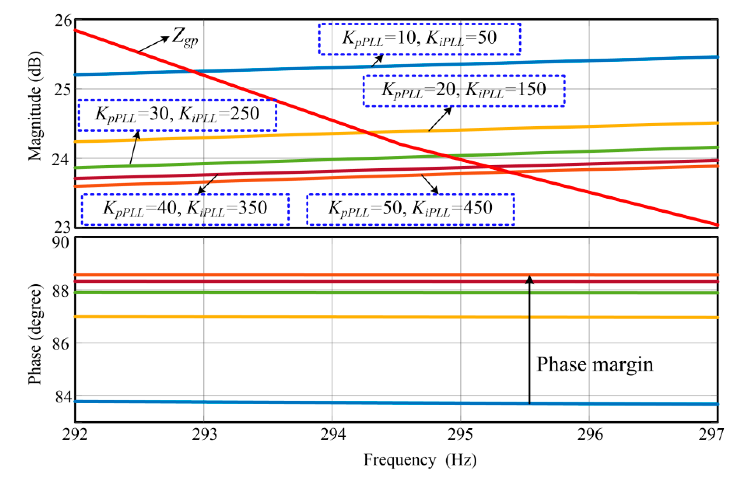
4.1. Simulation Results with SRF-PLL

Figure 9 shows the Bode plot of the closed loop transfer function of PLL with the parameters given in Table 1. It can be seen in Figure 9 that the PLL bandwidth with different parameters varies in direct proportion with the proportional and integral gains of PLL, resulting in low, medium, and high bandwidth PLL.

The Bode plot of parallel compensated weak grid impedance in (31) with (C_g2 = 0.0032 F and 0.0062 constituting Z_gp1 and Z_gp2), and the DFIG system impedance in (30) is shown in Figure 10.

It can be seen in Figure 10 that α component of DFIG impedance in pink has the magnitude intersection point with weak grid impedance at point A₁ and A₂. The corresponding phase difference at point A₁ and A₂ is less than 180°. Accordingly, the resonance at the middle frequency is not likely to occur. The reason is that there is no PLL involved in the α component of DFIG impedance. The β components of DFIG impedance while taking the low bandwidth PLL into consideration have the magnitude intersection points C₁ and C₂ with weak grid impedance. The phase differences at the corresponding points are less than 180°. The resonance at the middle frequencies is not likely to occur due to the low bandwidth of PLL. However, if the medium and high bandwidth PLL is taken into consideration, the β component of DFIG impedance has two magnitude intersection points with weak grid impedance, namely B₁ and B₂. Additionally, the corresponding phase difference at the point B₁ and B₂ are higher than 180° at frequencies 210 Hz and 290 Hz, respectively. This shows that the high bandwidth of PLL can cause resonance to occur at the middle frequencies, i.e., from 200 Hz to 800 Hz. The aforementioned analysis and simulation results show that PLL parameters have a significant impact on the resonance.

Figure 11 shows the Bode diagram with different SRF-PLL control parameters.

Choosing the small K_pPLL and K_iPLL for PLL, the high phase margin can be guaranteed, and the resonance is not likely to occur, as can be seen in Figure 11. However, when the PLL parameters are increased, i.e., the high bandwidth PLL can cause less phase margin, as shown in Figure 11. It is noteworthy that the DFIG system impedance does not rely on PLL impedance. Other parameters, like the digital delay of PWM and the parameters of the current controller, can also affect the impedance modeling of the DFIG system.

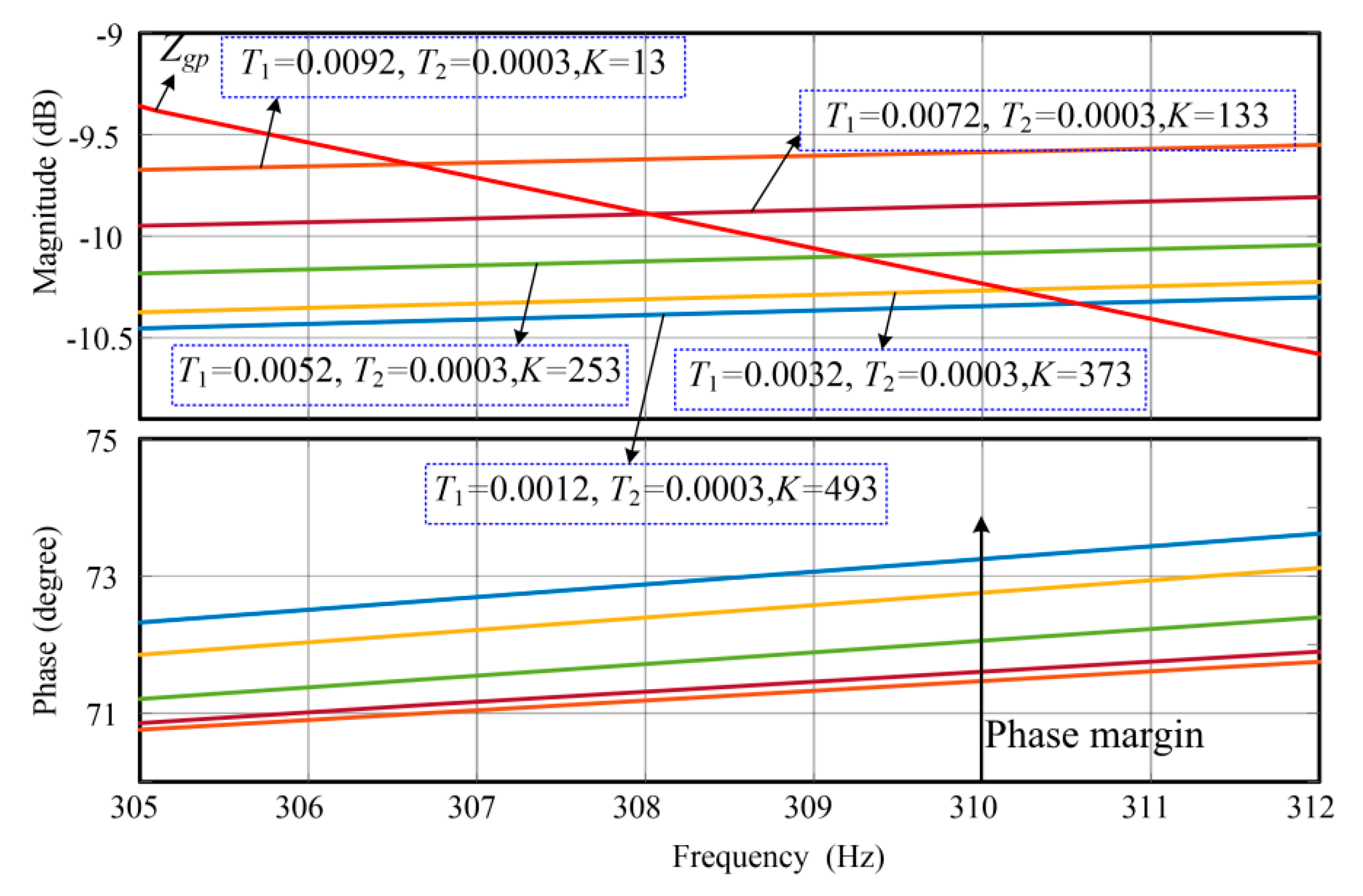
4.2. Simulation Results with Lead/Lag PLL

Selecting three different Lead/Lag PLL with the same bandwidth (low, medium, and high) as SRF-PLL and Lead/Lag PLL is shown in Figure 12. Table 1 provides the Lead/Lag PLL parameters.

The Bode plot of parallel compensated weak grid impedance in (31) (C_g2 = 0.0032 F and 0.0062 constituting Z_gp1 and Z_gp2), and the DFIG system impedance in (34) for three Lead/Lag PLL with different parameters is shown in Figure 13.

It can be seen in Figure 13 that α component of DFIG impedance in pink has the magnitude intersection point with weak grid impedance at point C₁ and C₂. The corresponding phase difference at point C₁ and C₂ is less than 180°. Accordingly, the resonance at the middle frequency is not likely to occur. The reason is that there is no PLL involved in the α component of DFIG impedance. The β component of DFIG impedance taking the low and high bandwidth Lead/Lag PLL into consideration have the magnitude intersection points A, A₁, and A₂ for grid impedance Z_gp2 and B, B₁, and B₂ for grid impedance Z_gp1. The phase differences at the corresponding points are less than 180°. The resonance at the middle frequencies is not likely to occur due to the low bandwidth of PLL. However, if the medium and high bandwidth PLL is taken into consideration, then the β component of DFIG impedance might cause resonance at middle frequencies. The aforementioned analysis and simulation results show that Lead/Lag PLL parameters have little impact on the impedance modeling of the DFIG system as compared to SRF-PLL.

Figure 14 depicts the Bode diagram with different Lead/Lag PLL control parameters to give a more clear insight into the resonance. It can be seen in Figure 14 that selecting the low bandwidth Lead/Lag PLL, the high phase margin can be guaranteed, and the resonance is not likely to occur. However, the high bandwidth Lead/Lag PLL can cause less phase margin, as shown in Figure 14. It is noteworthy, that phase margin taking high bandwidth Lead/Lag PLL is high when compared to SRF-PLL with high bandwidth.

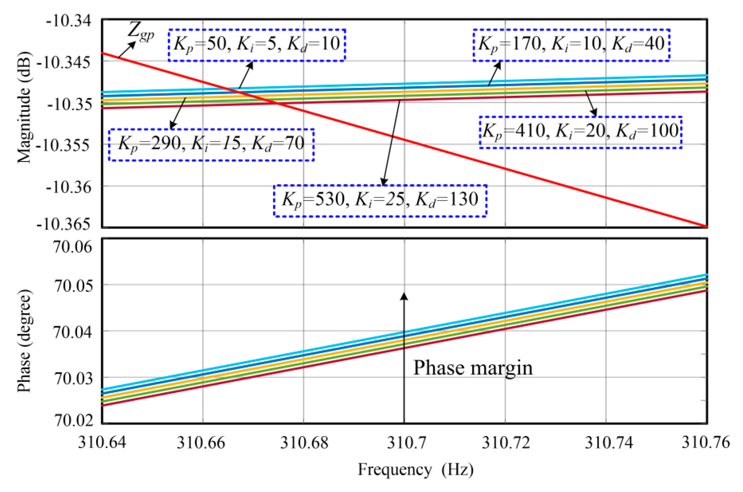
4.3. Simulation Results with Improved PLL

Figure 15 shows three different improved PLL with the same bandwidth (low, medium, and high) as SRF-PLL, and Lead/Lag PLL, with the parameters being given in Table 1.

Figure 16 depicts the Bode plot of parallel compensated weak grid impedance in (31) (C_g2 = 0.0032 F and 0.0062 F constituting Z_gp1 and Z_gp2), and the DFIG system impedance in (37).

Figure 16 shows that the α component of DFIG impedance in pink and the β component with low and high bandwidth improved PLL have approximately the same impedance shape. There exist two magnitude intersection points with weak grid impedance at points A and B. The corresponding phase difference at points A and B is less than 180°. Hence, the resonance at the middle frequency is not likely to occur, even with the high bandwidth improved PLL. The aforementioned analysis and simulation results show that improved PLL parameters have an insignificant impact on the DFIG system impedance modeling when compared to SRF-PLL and Lead/Lag PLL.

The Bode plot of parallel compensated weak grid, and the DFIG system with improved PLL of different control parameters is shown in Figure 17 to give a more clear insight into the resonance. Contrary to SRF-PLL and Lead/Lag PLL, the high phase margin can be guaranteed in the case of improved PLL. Additionally, it can be seen in Figure 17 that the control parameters of improved PLL have a minimal effect on the phase margin. Accordingly, the improved PLL can be used as an alternative to SRF-PLL and Lead/Lag PLL for the DFIG system under the weak grid to guarantee the improved dynamic performance and stability enhancement.

5. Time Domain Simulations

This section validates impedance modeling through time domain simulations.

5.1. Simulation Results with SRF-PLL

Two cases of low and high bandwidth SRF-PLL are validated through time-domain simulations. Figure 18a,b depict the stator voltage, stator and rotor current, active and reactive power, and torque for the DFIG system operated under weak grid employing the low bandwidth PLL (K_pPL = 5, K_iPLL = 50) and high bandwidth PLL (K_pPLL = 500, K_iPLL = 5000), respectively. With the low bandwidth PLL, the resonance at middle frequency will not exist, as can be seen in Figure 18a. Contrary to Figure 18a, the resonance is likely to exist, as can be seen in Figure 18b. The resonance frequency in the stator and rotor current induce resonance in the active and reactive power and electromagnetic torque.

Figure 19a,b show the FFT analysis of the DFIG stator voltage with low and high bandwidth PLL, respectively. There is no resonance at the middle frequencies, as can be seen in Figure 19a However, the resonance at 295 Hz and 3955 Hz exists if the high bandwidth SRF-PLL is considered, as reflected in Figure 19b.

5.2. Simulation Results with Lead/Lag PLL

Likewise, the SRF-PLL, Figure 20a, and Figure 20b depict the stator voltage, stator, and rotor current, active and reactive power, and torque employing the low bandwidth (K = 13, T₁ = 0.0092, T₂ = 0.0003) and high bandwidth (K = 493, T₁ = 0.0012, T₂ = 0.0003) Lead/Lag PLL, respectively. If the low bandwidth Lead/Lag PLL is chosen for the DFIG system, the resonance at middle frequency will not exist, as indicated in Figure 20a. Contrary to Figure 20a, the resonance is likely to exist in the aforementioned quantities, as demonstrated in Figure 20b.

Figure 21a,b portray the FFT analysis of the DFIG stator voltage with low and high bandwidth Lead/Lag PLL, respectively. It can be seen in Figure 21a that there is no resonance at the middle frequencies. However, the resonance at 305 Hz and 405 Hz occurs if the high bandwidth Lead/Lag PLL is considered, as evident in Figure 21b.

5.3. Simulation Results with Improved PLL

Two cases of low and high bandwidth improved PLL is validated through time domain simulations. Figure 22a, and Figure 22b show the stator voltage, stator and rotor current, active and reactive power, and torque for the DFIG system operated under weak grid employing the low bandwidth (K_pPLL = 50, K_iPLL = 5, K_dPLL = 10) and high bandwidth PLL (K_pPLL = 5000, K_iPLL = 500, K_dPLL = 1000) improved PLL, respectively. It can be seen in Figure 22a if the low bandwidth improved PLL is chosen for the DFIG system, the resonance at middle frequency will not exist. Contrary to the case of SRF-PLL and Lead/Lag PLL with high bandwidth, the resonance will not be likely to exist in stator voltage and current, rotor current, active and reactive power, and electromagnetic torque, as can be seen in Figure 22b.

Figure 23a,b demonstrate the FFT analysis of the DFIG stator voltage with low and high bandwidth improved PLL, respectively. The resonance does not exist at the middle frequencies, as reflected in Figure 23a. Similarly, the resonance at middle frequencies in the stator and rotor current, active and reactive power, and electromagnetic torque will not exist if the high bandwidth improved PLL is considered, as reflected in Figure 23b.

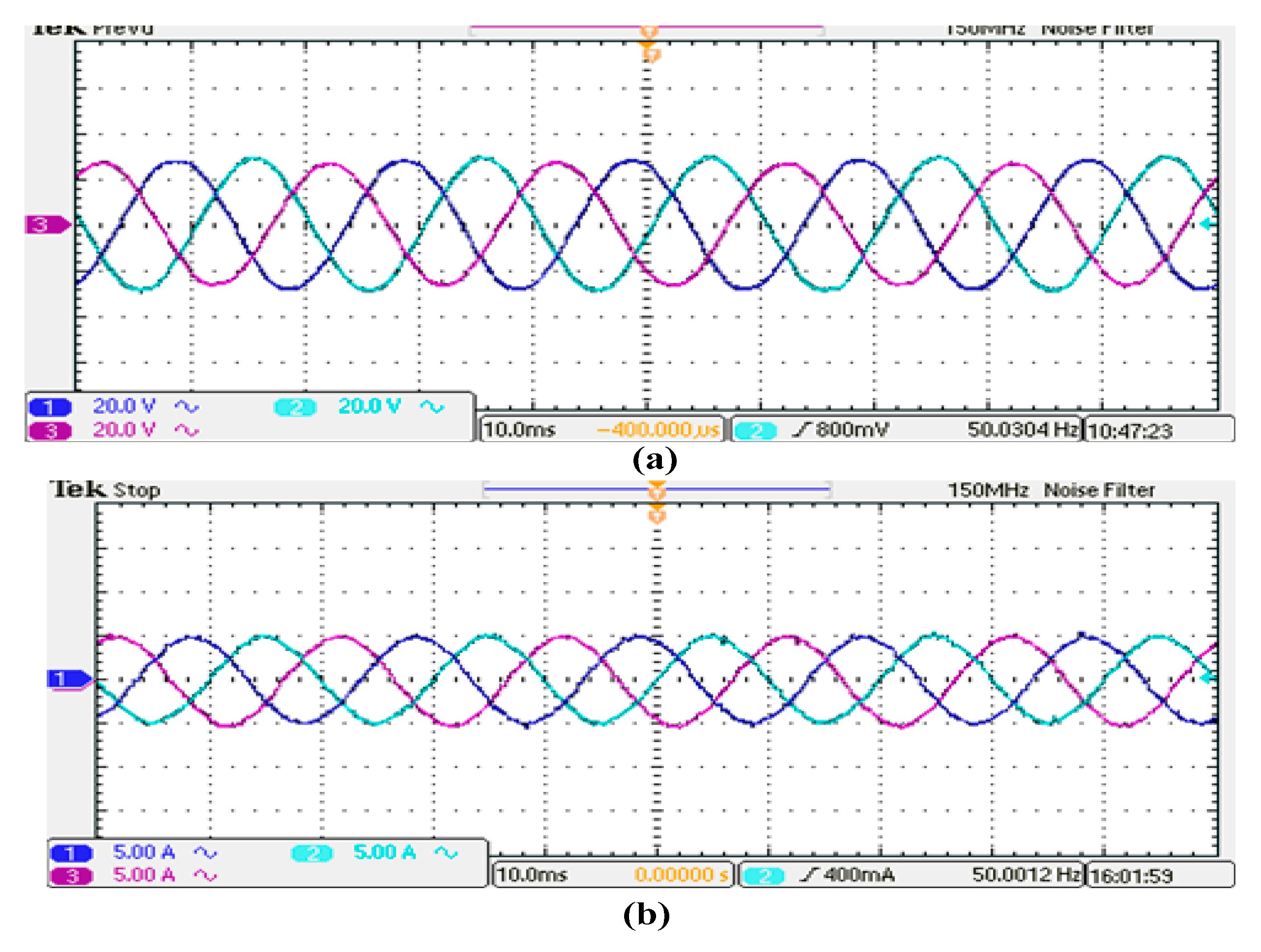
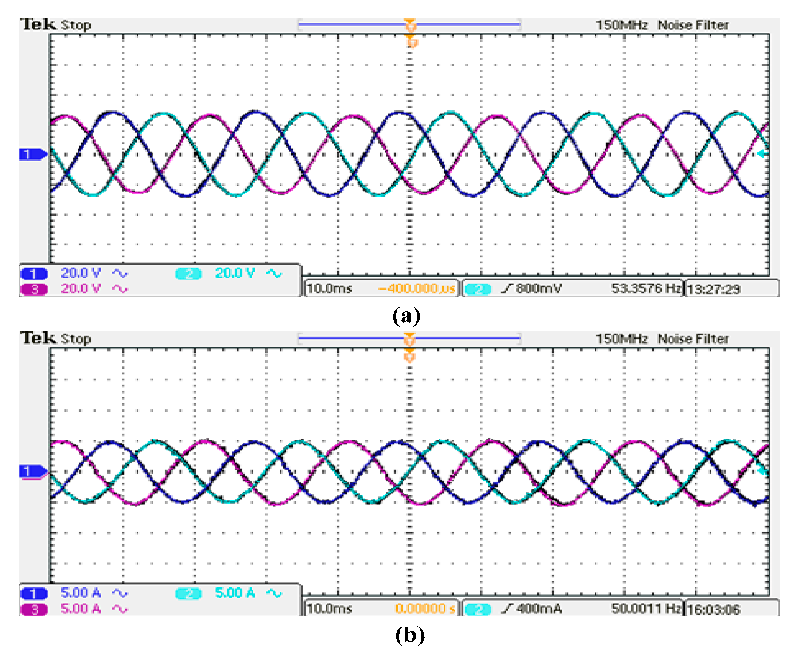
6. Experimental Results

The impact of PLL on the resonance in the DFIG system is validated while using the experimental setup, as shown in Figure 24.

The proportional and integral gain of three types PLL is the same as in Table 1. The experiments are conducted to show the stator voltage and stator current with low and high bandwidth SRF-PLL, Lead/Lag PLL, and an improved PLL. Similar results can be deduced for electromagnetic torque and active and reactive power, but it will not be discussed here in this paper.

Figure 25 and Figure 26 show the stator voltage and stator current of the DFIG system operated under a weak grid employing the low bandwidth PLL (K_pPLL = 5, K_iPLL = 50) and high bandwidth PLL (K_pPLL = 500, K_iPLL = 5000), respectively. With the low bandwidth PLL, the resonance at middle frequency will not exist in the DFIG stator voltage and stator current, as can be seen in Figure 25a,b. The resonance in the DFIG stator voltage and current is likely to exist, contrary to Figure 25a,b, as can be seen in Figure 26a,b, respectively.

Likewise, Figure 27 and Figure 28 show the stator voltage and stator current of the DFIG system operated under a weak grid employing the low bandwidth (K = 13, T₁ = 0.0092, T₂ = 0.0003) and high bandwidth (K = 493, T₁ = 0.0012, T₂ = 0.0003) Lead/Lag PLL, respectively. If the low bandwidth Lead/Lag PLL is chosen for the DFIG system, the resonance at middle frequency will not exist in the stator voltage and stator current, as can be seen in Figure 27a,b, respectively. The resonance in the DFIG stator voltage and stator current is likely to exist, contrary to Figure 27a,b, as can be seen in Figure 28a,b, respectively.

Similar to SRF and Lead/Lag PLL, the stator voltage and stator current with low bandwidth (K_pPLL = 50, K_iPLL = 5, K_dPLL = 10) and high bandwidth (K_pPLL = 5000, K_iPLL = 500, K_dPLL = 1000) are shown in Figure 29 and Figure 30b, respectively. It can be seen in Figure 29a,b that the resonance at middle frequency does not exist in the DFIG stator voltage and stator current with low bandwidth improved PLL. Contrary to the case of SRF-PLL and Lead/Lag PLL with high bandwidth, the resonance will not be likely to exist in stator voltage and stator current of the DFIG system, as can be seen in Figure 30a,b, when an improved PLL is taken into consideration.

The aforementioned experimental results validate the time domain simulations for the DFIG system operated in a weak grid with the inclusion of PLL. The experimental results have good agreement with time domain simulations.

7. Conclusions

This paper has studied the impact of PLL on resonance at the middle frequencies in the DFIG system under a weak grid. Firstly, the small signal model of two types of traditional PLL and an improved PLL is established. Secondly, the impedance model of the DFIG system, while considering the impact of the small signal model of PLLs, is established. Subsequently, based on the impedance modeling, the resonance at middle frequencies with different controller parameters and different types of PLL has been investigated. The conclusions could be drawn, as follows:

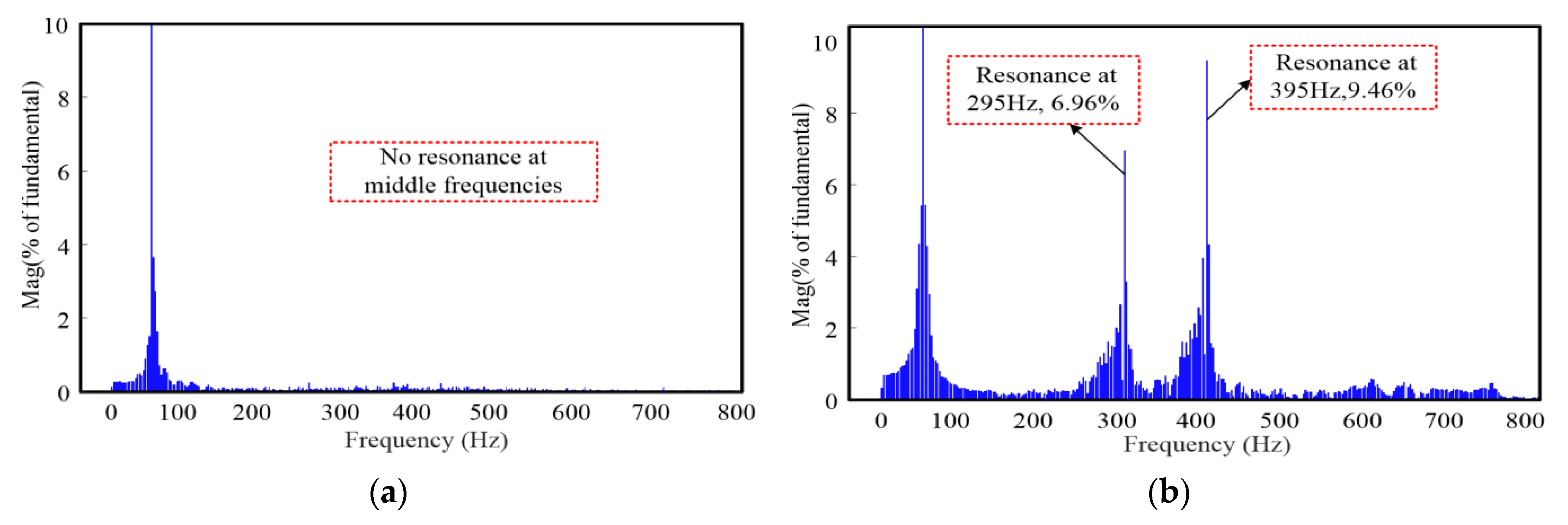
• The low bandwidth of any PLL (SRF, Lead/Lag, and improved) has no effect on the resonance at middle frequencies due to an acceptable phase margin.
• Resonance at middle frequencies exists in the DFIG system with high bandwidth SRF, and Lead/Lag PLL. However, there is no resonance at middle frequencies with the employment of improved PLL, even with the high bandwidth.
• The performance of the Lead/Lag PLL is superior to the same high bandwidth SRF-PLL due to the higher phase margin of the Lead/Lag PLL.
• The phase margin with the Lead/Lag PLL is less dependent on the PLL controller parameters as compared to SRF-PLL.
• The improved PLL controller parameters have an insignificant effect on the impedance modeling, as the phase margin is approximately the same for different bandwidth improved PLL.
• The α and β component DFIG system impedance with improved PLL has approximately the same impedance shape. Additionally, a high phase margin with improved PLL guaranteed better dynamic performance than the SRF-PLL and Lead/Lag PLL.
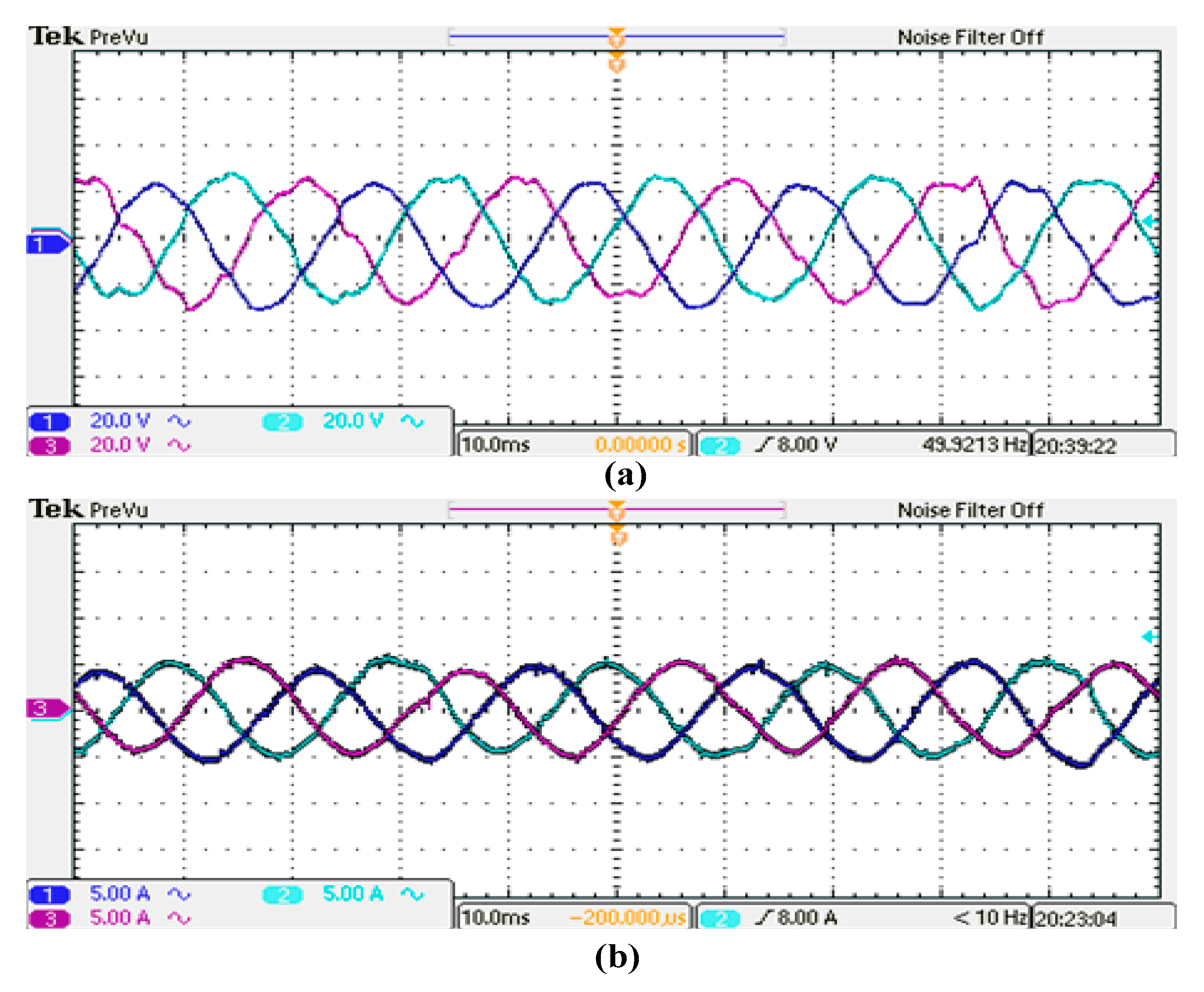
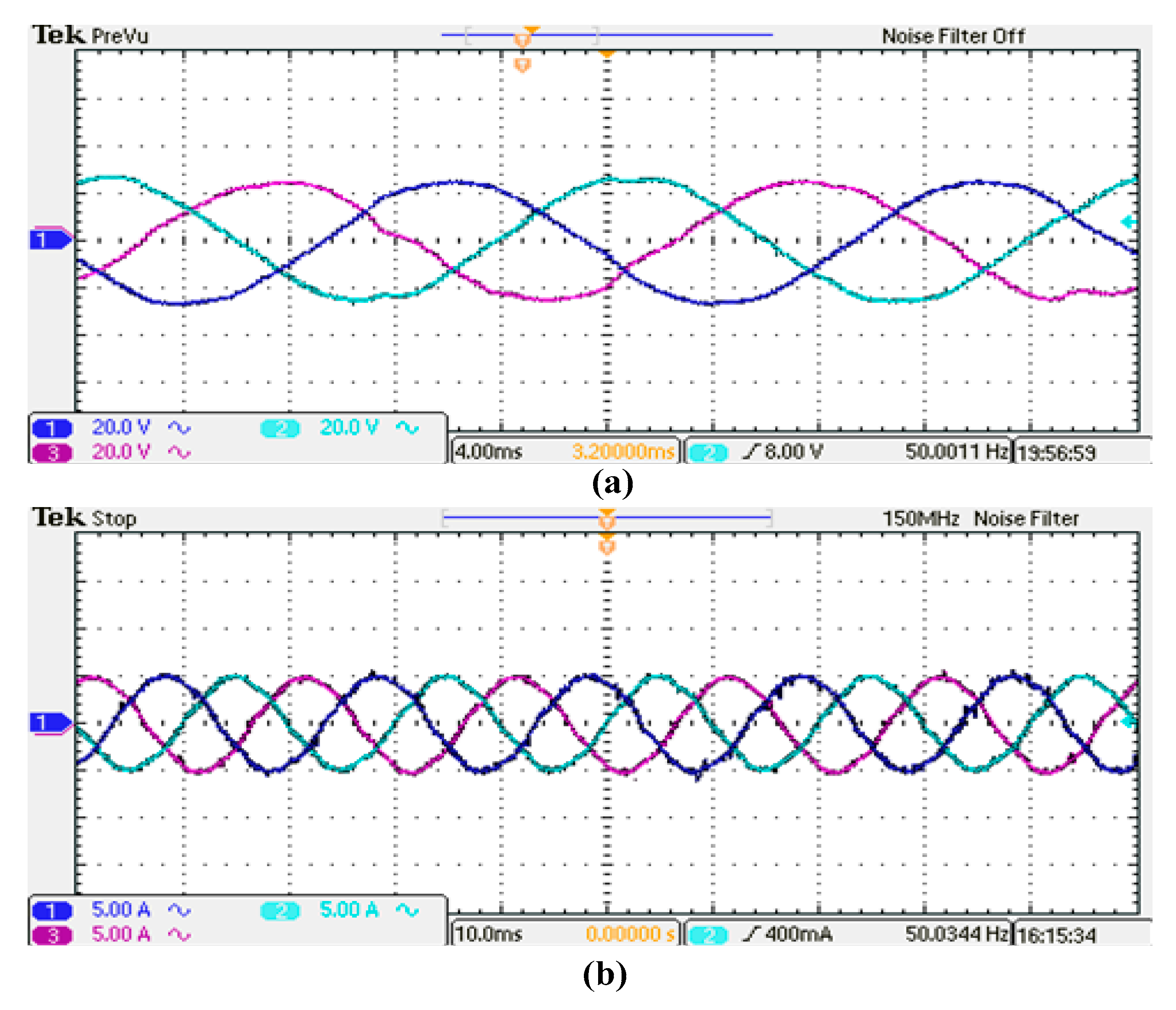
• The experimental results are in good agreement with the time domain simulations.

References

1. Müller, S.; Deicke, M.; Rik Doncker, D.W. Doubly fed induction generator systems for wind turbines. Ind. Appl. Mag. IEEE 2002, 8, 26–33. [Google Scholar] [CrossRef]
2. Cai, L.J.; Erlich, I. Doubly Fed Induction Generator Controller Design for the Stable Operation in Weak Grids. IEEE Trans. Sustain. Energy 2015, 6, 1078–1084. [Google Scholar] [CrossRef]
3. Grunau, S.; Fuchs, F.W. Effect of wind-energy power injection into weak grids. In Proceedings of the 2012 European Wind Energy Conference and Exhibition (EWEC), Copenhagen, Denmark, 16–19 April 2012; pp. 1150–1156. [Google Scholar]
4. Blaabjerg, F.; Ma, K. Future on power electronics for wind turbine systems. IEEE J. Emerg. Sel. Top. Power Electron. 2013, 1, 139–152. [Google Scholar] [CrossRef]
5. Vieto Sun, J. Sequence Impedance Modeling and Analysis of Type-III Wind Turbines. IEEE Trans. Energy Convers. 2018, 33, 537–545. [Google Scholar] [CrossRef]
6. Chen, W.; Xie, X.; Wang, D.; Liu, H.; Liu, H. Probabilistic stability analysis of subsynchronous resonance for series-compensated DFIG-based wind farms. IEEE Trans. Sustain. Energy 2018, 9, 400–409. [Google Scholar] [CrossRef]
7. Miao, Z. Impedance-model-based SSR analysis for type 3 wind generator and series-compensated network. IEEE Trans. Energy Convers. 2012, 27, 984–991. [Google Scholar] [CrossRef]
8. Zhang, X.; Zhang, Y.; Fang, R.; Xu, D. Impedance Modeling and SSR Analysis of DFIG Using Complex Vector Theory. IEEE Access 2019, 7, 155860–155870. [Google Scholar] [CrossRef]
9. Huang, P.; Shawky, M.; Moursi, E.; Xiao, W.; Member, S.; Kirtley, J.L. Subsynchronous Resonance Mitigation for Series-Compensated DFIG-Based Wind Farm by Using Two-Degree-of-Freedom Control Strategy. IEEE Trans. Power Syst. 2015, 30, 1442–1454. [Google Scholar] [CrossRef]
10. Du, W.; Ren, B.; Wang, H.; Wang, Y. Comparison of Methods to Examine Sub-Synchronous Oscillations Caused by Grid-Connected Wind Turbine Generators. IEEE Trans. Power Syst. 2019, 34, 4931–4943. [Google Scholar] [CrossRef]
11. Xie, X.; Zhang, X.; Liu, H.; Liu, H.; Li, Y.; Zhang, C. Characteristic Analysis of Subsynchronous Resonance in Practical Wind Farms Connected to Series-Compensated Transmissions. IEEE Trans. Energy Convers. 2017, 32, 1117–1126. [Google Scholar] [CrossRef]
12. Din, Z.; Zhang, J.; Zhang, Y.; Xu, Z.; Zhao, J.; Song, Y. Active damping of resonances in DFIG system with cascade converter under weak grid. Int. Trans. Electr. Energy Syst. 2019, 29, e12118. [Google Scholar] [CrossRef]
13. Song, Y.; Wang, X.; Blaabjerg, F. Impedance-Based High-Frequency Resonance Analysis of DFIG System in Weak Grids. IEEE Trans. Power Electron. 2017, 32, 3536–3548. [Google Scholar] [CrossRef] [Green Version]
14. Song, Y.; Blaabjerg, F. High-Frequency Resonance Damping of DFIG-Based Wind Power System UnderWeak Network. IEEE Trans. Power Electron. 2017, 32, 4370–4394. [Google Scholar] [CrossRef] [Green Version]
15. Song, Y.; Blaabjerg, F.; Wang, X. Analysis and Active Damping of Multiple High Frequency Resonances in DFIG System. IEEE Trans. Energy Convers. 2017, 32, 369–381. [Google Scholar] [CrossRef] [Green Version]
16. Din, Z.; Zhang, J.; Xu, Z.; Zhang, Y. Phase Angle Compensation of Virtual Impedance for Resonance Mitigation in DFIG System under Weak Grid. In Proceedings of the 8th IET International Conference on Renewable Power Generation (RPG 2019), Shanghai, China, 24–25 October 2019; pp. 1–8. [Google Scholar]
17. Nian, H.; Cheng, P.; Zhu, Z.Q. Independent operation of DFIG-based WECS using resonant feedback compensators under unbalanced grid voltage conditions. IEEE Trans. Power Electron. 2015, 30, 3650–3661. [Google Scholar] [CrossRef]
18. Jiang, Y.; Li, Y.; Tian, Y.; Wang, L. Phase-locked loop research of grid-connected inverter based on impedance analysis. Energies 2018, 11, 3077. [Google Scholar] [CrossRef] [Green Version]
19. Qian, Q.; Xie, S.; Xu, J.; Xu, K.; Bian, S.; Zhong, N. Output Impedance Modeling of Single-Phase Grid-Tied Inverters with Capturing the Frequency-Coupling Effect of PLL. IEEE Trans. Power Electron. 2019, 35, 5479–5495. [Google Scholar] [CrossRef]
20. Zhu, D.; Zhou, S.; Zou, X.; Kang, Y. Improved Design of PLL Controller for $LCL$-Type Grid-Connected Converter in Weak Grid. IEEE Trans. Power Electron. 2019, 35, 4715–4727. [Google Scholar] [CrossRef]
21. Wang, X.; Harnefors, L.; Blaabjerg, F. Unified Impedance Model of Grid-Connected Voltage-Source Converters. IEEE Trans. Power Electron. 2018, 33, 1775–1787. [Google Scholar] [CrossRef] [Green Version]
22. Wen, B.; Boroyevich, D.; Burgos, R.; Mattavelli, P.; Shen, Z. Analysis of D-Q Small-Signal Impedance of Grid-Tied Inverters. IEEE Trans. Power Electron. 2016, 31, 675–687. [Google Scholar] [CrossRef]
23. Wen, B.; Boroyevich, D.; Burgos, R.; Mattavelli, P.; Shen, Z. Small-Signal Stability Analysis of Three-Phase AC Systems in the Presence of Constant Power Loads Based on Measured d-q Frame Impedances. IEEE Trans. Power Electron. 2015, 30, 5952–5963. [Google Scholar] [CrossRef]
24. Wang, Y.; Chen, X.; Wang, Y.; Gong, C. Analysis of frequency characteristics of phase-locked loops and effects on stability of three-phase grid-connected inverter. Int. J. Electr. Power Energy Syst. 2019, 113, 652–663. [Google Scholar] [CrossRef]
25. Yang, D.; Wang, X.; Liu, F.; Xin, K.; Liu, Y.; Blaabjerg, F. Symmetrical PLL for SISO impedance modeling and enhanced stability in weak grids. IEEE Trans. Power Electron. 2020, 35, 1473–1483. [Google Scholar] [CrossRef]
26. Chou, S.-F.; Wang, X.; Blaabjerg, F. Two-Port Network Modeling and Stability Analysis of Grid-Connected Current-Controlled VSCs. IEEE Trans. Power Electron. 2019, 35, 3519–3529. [Google Scholar] [CrossRef]
27. Li, Y.; Fan, L.; Miao, Z. Wind in Weak Grids: Low-Frequency Oscillations, Subsynchronous Oscillations, and Torsional Interactions. IEEE Trans. Power Syst. 2019, 35, 109–118. [Google Scholar] [CrossRef]
28. Vieto Sun, J. Small-signal impedance modelling of type-III wind turbine. In Proceedings of the 2015 IEEE Power & Energy Society General Meeting, Denver, CO, USA, 26–30 July 2015; pp. 1–5. [Google Scholar]
29. Song, Y.; Blaabjerg, F. Analysis of Middle Frequency Resonance in DFIG System Considering Phase-Locked Loop. IEEE Trans. Power Electron. 2018, 33, 343–356. [Google Scholar] [CrossRef] [Green Version]
30. Zhan, C.; Fitzer, C.; Ramachandaramurthy, V.K.; Arulampalam, A.; Barnes, M.; Jenkins, N. Software phase-locked loop applied to dynamic voltage restorer (DVR). In Proceedings of the 2001 IEEE Power Engineering Society Winter Meeting, Conference Proceedings (Cat. No.01CH37194), Columbus, OH, USA, 28 January–1 Feberuary 2001; pp. 1033–1038. [Google Scholar]
Figure 1. Schematic diagram of the studied doubly fed induction generator (DFIG) system.
Energies 13 01039 g001
Figure 2. Schematic diagram of synchronous reference frame-phase locked loop (SRF-PLL).
Energies 13 01039 g002
Figure 3. Schematic diagram of Lead/Lag PLL.
Energies 13 01039 g003
Figure 4. Schematic diagram of improved PLL.
Energies 13 01039 g004
Figure 5. Schematic diagram of rotor side converter (RSC) rotor current control.
Energies 13 01039 g005
Figure 6. DFIG machine equivalent circuit (a) Overall; (b) simplified.
Energies 13 01039 g006
Figure 7. Simplified control diagram of GSC and LCL filter.
Energies 13 01039 g007
Figure 8. LCL filter equivalent circuit (a) Overall; (b) simplified.
Energies 13 01039 g008
Figure 9. Closed-loop frequency response of SRF-PLL.
Energies 13 01039 g009
Figure 10. Bode plot of DFIG impedance and parallel compensated weak grid with low, medium, and high bandwidth SRF-PLL.
Energies 13 01039 g010
Figure 11. Bode plot of DFIG impedance and parallel compensated weak grid with different PLL parameters.
Energies 13 01039 g011
Figure 12. The closed-loop frequency response of Lead/Lag PLL.
Energies 13 01039 g012
Figure 13. Bode plot of DFIG impedance and parallel compensated weak grid with low, medium, and high bandwidth Lead/Lag PLL.
Energies 13 01039 g013
Figure 14. Bode plot of DFIG impedance and parallel compensated weak grid with different Lead/Lag PLL parameters.
Energies 13 01039 g014
Figure 15. The closed-loop frequency response of improved PLL.
Energies 13 01039 g015
Figure 16. Bode plot of DFIG impedance and parallel compensated weak grid with low, medium, and high bandwidth improved PLL.
Energies 13 01039 g016
Figure 17. Bode plot of DFIG impedance and parallel compensated weak grid with different improved PLL parameters.
Energies 13 01039 g017
Figure 18. Simulation results of DFIG system in weak grid with SRF-PLL (a) Low bandwidth; and, (b) High bandwidth.
Energies 13 01039 g018
Figure 19. FFT analysis of stator voltage (a) Low bandwidth SRF-PLL; and, (b) High bandwidth.
Energies 13 01039 g019
Figure 20. Simulation results of DFIG system in weak grid with Lead/Lag PLL (a) Low bandwidth; and, (b) High bandwidth.
Energies 13 01039 g020aEnergies 13 01039 g020b
Figure 21. FFT analysis of stator voltage with Lead/Lag PLL (a) Low bandwidth; and, (b) High bandwidth.
Energies 13 01039 g021
Figure 22. Simulation results of DFIG system in weak grid with improved PLL (a) Low bandwidth, and (b) High bandwidth.
Energies 13 01039 g022
Figure 23. FFT analysis of stator voltage with improved PLL (a) Low bandwidth; and, (b) High bandwidth.
Energies 13 01039 g023
Figure 24. Experimental set up of the proposed DFIG system.
Energies 13 01039 g024
Figure 25. DFIG system in weak grid with low bandwidth SRF-PLL (a) Stator voltage, and (b) Stator current.
Energies 13 01039 g025
Figure 26. DFIG system in weak grid with high bandwidth SRF-PLL (a) Stator voltage, (b) Stator current.
Energies 13 01039 g026
Figure 27. DFIG system in weak grid with low bandwidth Lead/Lag PLL (a) Stator voltage, and (b) Stator current.
Energies 13 01039 g027
Figure 28. DFIG system in weak grid with high bandwidth Lead/Lag PLL (a) Stator voltage, and (b) Stator current.
Energies 13 01039 g028
Figure 29. DFIG system in weak grid with low bandwidth improved PLL (a) Stator voltage, and (b) Stator current.
Energies 13 01039 g029
Figure 30. DFIG system in weak grid with high bandwidth improved PLL (a) Stator voltage, and (b) Stator current.
Energies 13 01039 g030