Optimal Inventory Control Strategies for Deteriorating Items with a General Time-Varying Demand under Carbon Emission Regulations

Abstract

Climate warming nowadays has caused people to increasingly enhance public awareness about carbon emissions from industries. In the storing industry, inventory management for deteriorating items is crucial in the business competition. To slow down the deterioration and ensure the quality of products, the items are usually stored in certain temperature-controlled environment. However, a lot of carbon emissions of the inventory system are caused by these warehousing activities. In a finite panning period, this paper studies a continuous review inventory system and proposes inventory models to analyze the impacts of carbon emissions on inventory system for deteriorating items with a general time-varying demand, in which shortages are allowed, and the customer demand during shortage period is partially backlogged till the next replenishment. Under carbon emission regulations, the existence and uniqueness of the optimal solution to each model is explored and comparisons of optimality among the proposed models are given. Numerical examples and robust analysis of the models are presented to illustrate the applicability in practice. Some management insights about inventory policies and emission reduction strategies are obtained.

1. Introduction

Nowadays, with the globalization of service economy, enterprises often purchase, produce, distribute, maintain, and deliver goods across continents, and there has been a significant increase in the volume of worldwide trade [1]. Facing global customers, it must be quick and timely for enterprises to market products and services, which urges inventory managers to have to make a fine judgement [2]. To enhance the competitiveness of enterprises in the market, an adequate and proper planning of inventory replenishment is required for the effective coordination of the purchase, production, distribution, maintenance, and delivery of products to meet customer needs [3,4]. Thus, inventory service operation has became an important activity for enterprises in the business competition.

Inventory model, as a mean for quantitative analysis in inventory service operation, may help managers determine the optimal inventory replenishment strategy, which can be used to optimize inventory system costs associated with the storage and maintenance of products [5]. It is often assumed that the customer demand rate remains constant throughout the inventory cycle in some economic order quantity (EOQ) inventory models [6,7,8]. However, this basic assumption is often not true in some real situations, and inventory models may be more useful when the customer demand is not a constant, but changes with time [9]. When customer demand follows time distribution, there are some different ways that items are depleted from stock during the storage period. These ways are often referred to as demand patterns. Over the past few decades, many scholars have focused on inventory models with different demand patterns such as Linear demand [10,11], Quadratic demand [12], Exponential demand [13,14,15], and so on. Nevertheless, the impact of environmental factors on the inventory system has not been investigated in the aforementioned inventory problems with the time-varying demand.

In recent years, climate warming and frequent occurrences of natural disasters has made people increasingly aware of environmental issues. The Inter-governmental Panel on Climate Change (IPCC) reports that emissions of carbon dioxide from industrial and economic activities mainly give rise to global warming [16]. To slow down global warming, some countries and regional organizations, including the United Nations (UN), the European Union (EU), and China, have carried out legislation or emission regulations such as carbon cap and carbon market to reduce carbon emissions [17]. Under these emission regulations, enterprises must replan their operations to decrease carbon emissions [18]. For example, Hewlett-Packard indicated that they decreased carbon dioxide release to the air from 26.1 tonnes to 18.3 tonnes in 2010 by changing inventory operations [19]. It is also found that firms can achieve their goal of carbon emission reduction by adjusting their inventory, warehousing, and logistics operations [20]. Up to now, carbon emission issues caused by warehousing and logistic activities have received more and more attention from industry and academia [6].

In the inventory system, another realistic phenomenon is the deterioration of goods. As is well known, some items like refrigerated food, fresh food, vegetable, and fruit have a high deterioration rate during the storage period. To slow down the deterioration, these goods often need to be stored using temperature-controlled equipments [21]. It is found that the carbon footprint mainly stems from the use of cooled/refrigerated storage in the process of storing [8,22]. In the retail industry, it is reported by Walmart (http://www.walmartstores.com/sites/responsibility-report/2012/sustainableFacilities.aspx) that the refrigerants used in grocery stores accounted for a larger percentage of Walmart’s greenhouse gas footprint than its truck fleet, and similar case was confirmed in the report of Tesco (http://www.tesco.com/climatechange/carbonFootprint.asp). Therefore, in contrast to nonperishable items, carbon footprint management for the deterioration of inventory is more realistic in modern service operation. However, until now, the total effect of the deterioration and the time-varying demand on the measurable environmental performance is still an unexplored issue, which is exactly the focus of our study.

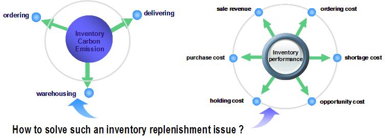
Toward this end, this paper quantifies the impact of emission regulations on the inventory model for deteriorating items with the time-varying demand. A novel model with sustainability for deterioration items under carbon emission regulations is investigated in the inventory system, in which carbon emissions caused by logistics and warehousing activities are considered, customer demands are assumed to be time-varying, and partial backlogging is allowed when the inventory system is out of stock. Specifically, the following research questions are addressed.

• How to determine the optimal replenishment strategy and emission reduction plan under carbon emission regulations?
• How do enterprises make the best choice when several carbon emission regulations coexist in the market?
• What is the effect of some important inventory characteristics such as deterioration, lost sales, carbon price, and carbon cap on the replenishment strategy of the inventory system?

The remainder of this paper is organized as follows. The related literature is reviewed in Section 2. The notations and assumptions related to this study are introduced in Section 3. Section 4 develops basic inventory model. Section 5 and Section 6 explore the models considering emission regulations. Then, the existence and uniqueness of the solution to the model are discussed and the comparison of optimality among the proposed models are given in Section 5, Section 6 and Section 7. In Section 7, the solution procedure of the models is illustrated through numerical examples, and in Section 8, robust analysis of the optimal solution with respect to major parameters is also carried out. The last section summarizes our contributions and discusses the directions of future research.

2. Literature Review

Our study is related to three streams in literatures for inventory issues. The first is on the inventory operation under the low carbon environment. As global commercial operation becomes increasingly conscious of low carbon concerns, many countries and regional organizations have launched low-carbon regulations to curb carbon emissions. When making business decisions, leading companies are also motivated to reduce carbon emissions by government’s low-carbon regulations such as the cap policy and the cap-and-trade policy [23]. Under the cap policy, enterprises are not allowed to exceed mandatory emission limits predetermined by the government. However, under the cap-and-trade policy, carbon emissions can be traded in the carbon market, i.e., this regulation sets a mandatory limit on emissions to all firms engaged in business activities and allows them to buy or sell carbon emission permits. Recently, especially in inventory operation, more and more scholars have focused on the effect of carbon emissions on inventory management. From the perspective of managing carbon footprints in inventory operation, Hua et al. [6] explored how firms optimize carbon footprints under the cap and trade policy, where the optimal order size is given and the effects of key parameters like the carbon cap and the carbon price on the inventory performance are discussed. Using the EOQ framework, Chen et al. [8] investigated a carbon-constrained inventory issue under carbon mechanisms including cap, carbon tax, and cap-and-offset. Toptal et al. [24] extended the EOQ model by taking into account emission reduction investments and analyzed joint decision-making of the inventory order policy and the emission reduction investment in the context of different carbon emission mechanisms. More recently, considering demand linked credit, Dye and Yang [25] developed a sustainable inventory model for deteriorating items with carbon emission constraints. In the manufacturing environment, Tang et al. [26] explored product configuration optimisation with customer satisfaction and low carbon constraints. Xu et al. [27] further discussed inventory models for deteriorating items with the inventory-dependent consumption rate and investigated the effect of carbon emission regulations on inventory performances. From the perspective of supply chain integration, Shen et al. [28] explored a production inventory issue for deteriorating items with collaborative preservation technology investment under a carbon tax policy. Additionally to providing inventory models for studying the replenishment policy of deteriorating items, this paper will also focus on two carbon emission regulations, i.e., the carbon cap policy and the cap and trade policy, as well as the comparison of optimality among the proposed models.

The second stream is on the time-varying demand pattern, as this paper will explore how to make order decisions within a finite planning period when customer demands change with time. Recently, the growth of modern commercial activities have prompted the research on inventory management to meet customer demands. Within the EOQ framework, some extensions to existing inventory models have been explored. Among them, a very interesting extension is the consideration of time-varying demands, which has attracted much attention from academia. For example, Silver and Meal [9] were the first who explored the inventory problems with time varying demands. Donaldson [10] gave an analytical solution to the inventory model with a linear demand trend. Bose et al. [11] also investigated an EOQ model with the linear time-dependent demand and provided an inventory replenishment policy considering allowing shortages and time value of money. Later, EOQ models with the power time-dependent demand was considered by [13,14,15,29]. However, customer demands cannot always increase continuously with time. For instance, the demand rate for some season or fad products increases with time initially, then keeps steady, and finally decreases over time. Considering partial backlogging and the Weibull deterioration rate, Skouri et al. [30] studied inventory models with the general ramp type demand rate under two different inventory systems including beginning with no shortages and beginning with shortages. More recently, Sarkar et al. [12] extended the model of Ghosh and Chaudhuri [31] by investigating an inventory issue for deteriorating products with the time dependent quadratic demand rate and shortages. In the case that shortages are completely backlogged within a fixed order cycle, Cheng and Wang [32] proposed the model with a constant deterioration and trapezoidal type demand. Taking into account the price-sensitive trapezoidal time varying demand and net credit, Shah et al. [33] further developed a joint supplier-buyer inventory model. In a finite time horizon, Wang et al. [34] explored an inventory policy with time-varying demand and deteriorating item under trade credit and inflation. Xu et al. [35] discussed a two-warehouse inventory decision model for a nonperishable product with a generalized trapezoidal-type time-varying demand rate. However, the impact of carbon emission regulations on the inventory system has been ignored in the above researches.

The third stream is on the deterioration inventory issues, in which inventory models for deteriorating items have been continuously extended by more and more scholars so as to reflect more realistic inventory characteristics. As declared in literatures, deterioration phenomena during the storage period are damage, decay, evaporation, spoilage, pilferage, dryness, and so on. Once the deterioration phenomena occurs in the retail inventory system, the loss of commodity utilities may result in decreased usefulness. In real life, many physical goods such as fresh fruits and vegetables, medicine, and blood banks often undergo spoilage or decay over time. In academia, Ghare and Schrader [36] made the first attempt to describe a decaying inventory system, in which the deteriorating rate is assumed to follow the exponential time-varying distribution. Covert and Philip [37] investigated an inventory issue with two-parameter Weibull distributed deterioration. Later, some scholars gave reviews of researches about deteriorating goods in different historical periods. For instance, Nahrnias [38] summarized early works on deteriorating commodities. Based on different inventory environments, such as single and multiple products, deterministic and stochastic demand, quantity discount, and time value of money, Raafat [39] cataloged literatures on perishable commodities in the 1980s. Goyal and Giri [40] provided a detailed review on the deteriorating inventory in the last decade of the 20th century, during which the main concern of scholars is to combine the deteriorating inventory management with supply chain management, information asymmetry, stochastic environment, and other cases. Recently, Bakker et al. [41] gave a up-to-date review in the field of the deteriorating inventory since 2001 by investigating system characteristics such as price discounts, single or multiple items, single or multi-echelon, one or multi-warehouse, and so on. Considering three-parameter Weibull distributed deterioration, Yang [42] discussed a two-warehouse inventory replenishment policy with partial backlogging under inflation. Under two different contracts including cost sharing and two-part tariff, Bai et al. [43] investigated a sustainable supply chain coordination issue with deteriorating items. In contrast to these works, this paper will consider a deteriorating inventory system in which shortages are allowed and the unsatisfied order will be partially backlogged under carbon emission regulations.

3. Assumptions and Notations

• Basic inventory description

As shown in Figure 1, a continuous review inventory system running in a finite panning period is considered. Items ordered are perishable in the system, where there is no repair or replenishment of the deteriorated inventory. It is assumed that the items deteriorate at a time-varying rate $\theta (t)$, where $0<\theta (t)<1$. The replenishment rate is infinite and the lead time is zero. At the beginning of the inventory cycle, the items from stock are depleted due to the customer demand and the deterioration. When the inventory level reaches zero, shortages occur in the inventory system. As some customers are unwilling to wait backlogged orders during the shortages period, the unsatisfied demand will only be backlogged partially in the next replenishment. Thus, the backlogging rate is adopted to describe this phenomenon as $\lambda (t)=D(t)+\delta I(t)$, where $D(t)$ denotes the customer demand, $I(t)$ denotes the inventory level during the shortage period, $\delta \ge 0$, and $I(t)<0$. Namely, the backlogging rate $\lambda (t)$ depends on the amount of the negative inventory $I(t)$, which implies that the more cumulative customers in the waiting line, the more scale of lost sales. This backlogging rate function is widely adopted in literatures [44].

• Inventory system’s carbon emission assumption

As some theoretical and practical studies have observed, delivering and storing items in practice consume significant amounts of energy, resulting in the creation of large amounts of carbon footprints from the transportation and inventory operations [45,46]. Thus, we focus on the carbon footprint caused by logistics and warehousing activities in our model.

The following model parameters, model operators, and decision variables are used throughout the paper.

• Model Parameters:
  K is the fixed cost incurred by per order;
  p is the selling price per unit;
  c is the purchasing cost per unit, and $p>c$;
  h is the holding cost per unit per unit time;
  $c_1$ is the lost sales per unit;
  $c_2$ is the shortage cost per unit per unit time;
  T is the fixed inventory cycle, namely, the length of inventory replenishment;
  S is the maximum shortages per cycle;
  L is the amount of lost sales per cycle;
  $\widehat{K}$ is the amount of the carbon emissions per order;
  $\widehat{h}$ is the amount of the carbon emissions incurred by per unit holding inventory per unit time;
  $\widehat{c}$ is the amount of the carbon emissions incurred by per unit of delivering;
  $c_p$ is the carbon price per unit carbon emission;
  $\widehat{E}$ is the capacity of the carbon emissions mandated by the government;
  $I_1(t)$ is the on-hand inventory level at time t in the stored period $[0,t_1]$;
  $I_2(t)$ is the negative inventory level at time t in the shortage period $[t_1,T]$;
  $\theta (t)$ is the time-varying deteriorating rate when the inventory system is on-hand;
  $D(t)$ is the time-varying demand rate, which is a general continuous function of time, and is positive in any given time horizon.

• Model Operators:
  $Tp(·)$ is the operator of the total profit for inventory system in $[0,T]$;
  $E(·)$ is the operator of the total carbon emissions associated behavior of the on-hand inventory;
  ${\Pi }_1(·)$ is the operator of the total profit without considering carbon emissions;
  ${\Pi }_2(·)$ is the operator of the total profit under the carbon cap policy;
  ${\Pi }_3(·)$ is the operator of the total profit under the carbon cap and trade policy.

• Decision Variables:
  $t_1$ is the time point when the on-hand inventory level drops to zero;
  Q is the order quantity per cycle.

4. Basic Model

Based on the above assumptions and description, it can be seen from Figure 1 that the inventory level $I_1(t)$ decreases due to the joint effects of the time varying demand and deterioration in $[0,t_1]$, whereas in $[t_1,T]$, $I_2(t)$ is at the negative inventory level, and the customer demand are only partially satisfied due to lost sales. Therefore, the variation of the inventory level can be described by the following equation,

$$\left\{\begin{array}{cc}\frac{\mathrm{d}{I}_1(t)}{\mathrm{d}t}=-D(t)-\theta (t)I_1(t),\hfill & 0\le t\le t_1;\hfill \\ \frac{\mathrm{d}{I}_2(t)}{\mathrm{d}t}=-D(t)-\delta I_2(t),\hfill & t_1\le t\le T,\hfill \end{array}\right.$$

(1)

with the boundary condition $I_1(t_1)=I_2(t_1)=0$. By solving the Equation (1), we get

$$\left\{\begin{array}{cc}{I}_1(t)={\int }_t^{t_1}{e}^{g(u)-g(t)}D(u)du,\hfill & 0\le t\le t_1;\hfill \\ I_2(t)={\int }_t^{t_1}{e}^{\delta (u-t)}D(u)du,\hfill & t_1\le t\le T,\hfill \end{array}\right.$$

(2)

where $g(z)={\int }_0^z\theta (m)dm$.

From Equation (2), the maximum shortages and the order quantity per cycle are obtained as follows,

$$S=-I_2(T)={\int }_{t_1}^T{e}^{-\delta (T-u)}D(u)du,$$

(3)

and

$$Q=I_1(0)+S={\int }_0^{t_1}{e}^{g(u)}D(u)du+{\int }_{t_1}^T{e}^{-\delta (T-u)}D(u)du.$$

(4)

Consequently, the amount of lost sales during the shortage period is shown as

$$L={\int }_{t_1}^{T}D(u)du-S={\int }_{t_1}^T(1-e^{-\delta (T-u)})D(u)du.$$

(5)

Thus, considering the inventory operation performance including sale revenue, the purchase cost, the holding cost, the opportunity cost due to lost sales, the shortage cost, and ordering cost, the total profit per cycle can be written as

$$\begin{array}{ccc}Tp(t_1)\hfill & =\hfill & p[{\int }_0^{t_1}D(u)du+S]-cQ-h{\int }_0^{t_1}{I}_1(t)dt-c_{1}L-c_2{\int }_{t_1}^T-I_2(t)dt-K\hfill \\ \hfill & =\hfill & p{\int }_0^{t_1}D(u)du+(p-c){\int }_{t_1}^T{e}^{-\delta (T-u)}D(u)du-c{\int }_0^{t_1}{e}^{g(u)}D(u)du\hfill \\ \hfill & -\hfill & h{\int }_0^{t_1}{\int }_t^{t_1}{e}^{g(u)-g(t)}D(u)dudt-c_1{\int }_{t_1}^T[1-e^{-\delta (T-u)}]D(u)du\hfill \\ \hfill & -\hfill & \frac{c_2}{\delta }{\int }_{t_1}^T[1-e^{-\delta (T-u)}]D(u)du-K.\hfill \end{array}$$

(6)

In addition, considering the inventory system’s carbon footprint including the carbon emissions incurred by delivering, warehousing, and fixed carbon emissions per order, the amount of carbon emissions per inventory cycle can be calculated as

$$\begin{array}{ccc}E(t_1)\hfill & =\hfill & \widehat{c}Q+\widehat{h}{\int }_0^{t_1}{I}_1(u)du+\widehat{K}\hfill \\ \hfill & =\hfill & \widehat{c}[{\int }_0^{t_1}{e}^{g(u)}D(u)du+{\int }_{t_1}^T{e}^{-\delta (T-u)}D(u)du]\hfill \\ \hfill & +\hfill & \widehat{h}{\int }_0^{t_1}{\int }_t^{t_1}{e}^{g(u)-g(t)}D(u)dudt+\widehat{K}.\hfill \end{array}$$

(7)

Therefore, combining Equation (6) with the above discussions, the optimization problem in the base inventory system without considering carbon emissions can be described as

$$\begin{array}{c}\mathrm{M}1:max{\Pi }_1(t_1)=Tp(t_1)\hfill \\ \mathrm{s}.\mathrm{t}.0\le t_1\le T.\hfill \end{array}$$

(8)

To solve Problem (8), calculate the first derivative of ${\Pi }_1(t_1)$, and we have $\frac{\mathrm{d}{\Pi }_1(t_1)}{\mathrm{d}{t}_1}=\frac{\mathrm{d}Tp(t_1)}{\mathrm{d}{t}_1}=F(t_1)D(t_1)$, where $F(t_1)=\frac{\delta (p+c_1)+c_2}{\delta }[1-e^{-\delta (T-t_1)}]-c[e^{g(t_1)}-e^{-\delta (T-t_1)}]-h{\int }_0^{t_1}{e}^{g(t_1)-g(t)}dt$. As $D(t_1)>0$, the optimal behavior of $Tp(t_1)$ only depends on the auxiliary function $F(t_1)$ during the time interval $[0,T]$. $F^{\prime }(t_1)=-[\delta (p+c_1-c)+c_2]e^{-\delta (T-t_1)}-\theta (t_1)e^{g(t_1)}[c+h{\int }_0^{t_1}{e}^{-g(u)}du]-h<0$ implies that $F(t_1)$ is a strictly monotone decreasing function in any given time interval. Therefore, the following theorem can be summarized for determining the optimal solution to M1.

Theorem 1.

In M1, for the above basic model with total profit ${\Pi }_1(t_1)$, there exits a unique optimal solution $t_1^{*}\in (0,T)$ such that $F(t_1)=0$.

Proof. 

Through simple derivation, we can get $F(0)=\frac{\delta (p+c_1-c)+c_2}{\delta }(1-e^{-\delta T})>0$ and $F(T)=-c[e^{g(T)}-1]-h{\int }_0^T{e}^{g(T)-g(t)}dt<0$. Recalling that $F(t_1)$ is a strictly monotone decreasing function with respect to $t_1$, Intermediate Value Theorem implies that there exits a unique root $t_1^{*}\in (0,T)$ satisfying $F(t_1^{*})=0$. Furthermore, taking the second derivative of $Tp(t_1)$ with respect to $t_1$, we have $\frac{{\mathrm{d}}^{2}Tp(t_1)}{\mathrm{d}{t}_1^2}{|}_{t_1=t_1^{*}}=D(t_1^{*})F^{\prime }(t_1^{*})<0$. According to the second order sufficient condition, it can be concluded that $t_1^{*}$ is the unique maximum value point of $Tp(t_1)$. □

Theorem 1 indicates that the optimal time point $t_1^{*}$ in the inventory system is unique and satisfies the equation $F(t_1)=0$, which makes the finding of the optimal solution to M1 easier. Meanwhile, we can easily get $Q^{\prime }(t_1)>0,S^{\prime }(t_1)<0$, and $L^{\prime }(t_1)<0$ from Formulas (3)–(5), which indicates that the order quantity increases as $t_1$ increases, whereas the maximum shortages and the amount of lost sales decrease as $t_1$ increases. The results are intuitively consistent. That is, in the fixed inventory cycle, the more larger the value of $t_1$, the more higher on-hand inventory level. Although the shortage level keeps smaller in the stockout period, it will make the waiting customers become more loyal due to the improvement of service level.

5. The Inventory Model under the Carbon Cap Mechanism

In the carbon cap model, the government sets a mandatory quota $\widehat{E}$ on the amount of pollution that the inventory enterprises can emit in a given period. Under this limitation, inventory managers need to determine the optimal ordering quantity for maximizing their total profit at the beginning of the inventory cycle. By combining Equations (6) and (7), the optimization problem in the inventory system can be described as follows,

$$\begin{array}{c}\mathrm{M}2:max{\Pi }_2(t_1)=Tp(t_1)\hfill \\ \mathrm{s}.\mathrm{t}.E(t_1)\le \widehat{E},\hfill \\ 0\le t_1\le T.\hfill \end{array}$$

(9)

The following theorem is provided for determining the optimal solution to M2.

Theorem 2.

In M2, let $E(\widehat{t_1})=\widehat{E}$, and we have

(1) 

if $\widehat{t_1}\ge T$, then the optimal solution of M2 is equivalent to that of M1;

(2) 

if $\widehat{t_1}<T$, then the optimal solution of M2 is the same as that of M1 when $F(\widehat{t_1})<0$, and $t_1^{*}=\widehat{t_1}$ when $F(\widehat{t_1})\ge 0$.

Proof. 

(1)

If $T\le \widehat{t_1}$, the mandatory quota $\widehat{E}$ from the government is met automatically and the carbon cap is not binding. Thus, the optimal solution of M2 is equivalent to that of M1;

(2)

Let $\widehat{t_1}<T$. When $F(\widehat{t_1})<0$, following the proof of Theorem 4.1, we can get a unique root $t_1^{*}\in (0,\widehat{t_1})\subset (0,T)$ such that $F(t_1^{*})=0$. When $F(\widehat{t_1})\ge 0$, $\frac{\mathrm{d}{\Pi }_2(t_1)}{\mathrm{d}{t}_1}=\frac{\mathrm{d}Tp(t_1)}{\mathrm{d}{t}_1}=F(t_1)D(t_1)>F(\widehat{t_1})D(t_1)\ge 0$, which indicates that $Tp(t_1)$ is an increasing function of $t_1$ in the time interval $[0,\widehat{t_1}]$. Thus, $t_1^{*}=\widehat{t_1}$.

 □

Under the carbon cap mechanism, the optimal solution to M2 is dependent on the carbon cap $\widehat{E}$ and the sign of $F(\widehat{t_1})$ especially when $\widehat{t_1}<T$ and $F(\widehat{t_1})\ge 0$, which is different from the case for M1. The optimal behavior of the inventory system is absolutely determined by the government’s carbon cap, which implies that the government can make inventory managers become more rational by imposing appropriate carbon quota. In what follows, we will discuss how does the carbon cap affect the inventory operation performances.

The Effect of the Carbon Cap

Theorem 3.

Let $E^{NC}$ be the optimal carbon emissions without considering the carbon emission quota. For M2, both the optimal total profit and the optimal carbon emissions increase first, and then keep unchanged as the carbon cap increases.

Proof. 

When $\widehat{E}\le E^{NC}$, the optimal solution to M2 happens at the boundary point $t_1^{*}=\widehat{t_1}$, where $E(\widehat{t_1})=\widehat{E}$. Thus, the optimal total profit and carbon emissions increase as the carbon cap $\widehat{E}$ increases. When $\widehat{E}>E^{NC}$, the optimal solution to M2 occurs at an interior point in the feasible interval $(0,T)$. Then, the optimality in M2 is independent of the carbon cap $\widehat{E}$, i.e., the carbon cap is not binding. Thus, the optimal total profit and carbon emissions keep constant as the carbon cap increases. □

Theorem 3 shows that, on one hand, the government or policy makers can achieve the effect of reducing emissions by setting an appropriate carbon quota (i.e., $\widehat{E}\le E^{NC}$), instead of failure in the total control of carbon (i.e., $\widehat{E}>E^{NC}$); on the other hand, under the carbon cap mechanism, inventory managers can also maximize their profits by adjusting order and storage (i.e., $\widehat{E}\le E^{NC}$). Next, a comparison between M1 and M2 is given.

Theorem 4.

Let $Q^{NC}$ and $T{P}^{NC}$ be the optimal order quantity and the optimal total profit without considering any carbon emission limits, and $Q^{CC}$, $E^{CC}$, and $T{P}^{CC}$ be the optimal order quantity, the optimal carbon emissions, and the optimal total profit under the carbon cap, respectively. Compared with M1, we have

(1) 

$Q^{NC}\ge Q^{CC}$;

(2) 

$T{P}^{NC}\ge T{P}^{CC}$; and

(3) 

$E^{NC}\ge E^{CC}$.

Proof. 

By Theorem 2, when $\widehat{t_1}\ge T$, or when $\widehat{t_1}<T$ and $F(\widehat{t_1})<0$, the cap remains at a higher level, and this limitation is not binding. Then, the optimal ordering policy with the cap is the same as that without considering carbon emissions, that is, $Q^{NC}=Q^{CC}$, $T{P}^{NC}=T{P}^{CC}$, and $E^{NC}=E^{CC}<\widehat{E}$. However, when $\widehat{t_1}<T$ and $F(\widehat{t_1})\ge 0$, Theorem 1 shows that the cap is low. Under this restriction, the optimal time point only happens at $t_1^{*}=\widehat{t_1}$. Noting the monotonicity of $Q(t_1)$ and $TP(t_1)$, we get $Q^{CC}<Q^{NC}$, $T{P}^{NC}>T{P}^{CC}$, and $E^{NC}>E^{CC}=\widehat{E}$. In summary, we obtain that $Q^{NC}\ge Q^{CC}$, $T{P}^{NC}\ge T{P}^{CC}$, and $E^{NC}\ge E^{CC}$. □

Theorem 4 indicates that the carbon emission reduction can be achieved under the cap policy, but the total profit in M2 is less than or equal to that in M1. Thus, the inventory decision-maker may have little incentive to accept this amount of emission reduction in a mandatory manner adopted in M2.

6. The Inventory Model under the Cap and Trade Mechanism

The cap and trade mechanism, as one of the most effective market-dependent mechanisms, has been adopted by many countries and regions in the world. This mechanism also sets a mandatory quota $\widehat{E}$ on the amount of pollution to related industries in a given period, but different from the carbon cap mechanism in Section 5, it allows the firms to buy or sell any carbon credit within this quota from the external carbon market. In this section, let $X=E(t_1)-\widehat{E}$, where $X>0$ $(or<0)$ means that the inventory firm buys (or sells) the corresponding carbon credit from the market, and $X=0$ means the inventory firm neither buy or sell any credit in the carbon market. Therefore, the model with the cap and trade in the inventory system can be formulated as

$$\begin{array}{c}\mathrm{M}3:max{\Pi }_3(t_1)=Tp(t_1)-c_{p}X\hfill \\ \mathrm{s}.\mathrm{t}.0\le t_1\le T.\hfill \end{array}$$

(10)

Combining with Equations (6) and (7), the objective function in M3 can be written as

$$\begin{array}{ccc}{\Pi }_3(t_1)\hfill & =\hfill & p{\int }_0^{t_1}D(u)du+(p-c-c_p\widehat{c}){\int }_{t_1}^T{e}^{-\delta (T-u)}D(u)du-(c+c_p\widehat{c}){\int }_0^{t_1}{e}^{g(u)}D(u)du\hfill \\ \hfill & -\hfill & (h+c_p\widehat{h}){\int }_0^{t_1}{\int }_t^{t_1}{e}^{g(u)-g(t)}D(u)dudt-c_1{\int }_{t_1}^T[1-e^{-\delta (T-u)}]D(u)du\hfill \\ \hfill & -\hfill & \frac{c_2}{\delta }{\int }_{t_1}^T[1-e^{-\delta (T-u)}]D(u)du-(K+c_p\widehat{K})+c_p\widehat{E}.\hfill \end{array}$$

(11)

To solve M3, calculate the first derivative of ${\Pi }_3(t_1)$, and then we have $\frac{\mathrm{d}{\Pi }_3(t_1)}{\mathrm{d}{t}_1}=G(t_1)D(t_1)$, where $G(t_1)=\frac{\delta (p+c_1)+c_2}{\delta }[1-e^{-\delta (T-t_1)}]-(c+c_p\widehat{c})[e^{g(t_1)}-e^{-\delta (T-t_1)}]-(h+c_p\widehat{h}){\int }_0^{t_1}{e}^{g(t_1)-g(t)}dt$. Thus, the following conclusion can be derived.

Theorem 5.

In M3, for the total function ${\Pi }_3(t_1)$, there exits a unique optimal time point $t_1^{*}\in (0,T)$ satisfying $G(t_1)=0$.

Proof. 

As the proof is similar to that of Theorem 1, we leave the proof to the reader. □

Remark 1.

Theorems 1 and 5 also show that the optimal inventory decision is independent of any time-varying demand type. These findings are consistent with [47], who investigated inventory models with completely backlogging from the perspective of operation cost analysis. As carbon emission constraints are not considered in [47], our result can be regarded as a generalization of his work in this perspective. Next, the effect of the cap and the carbon price on the inventory operation performance is analyzed under the cap and trade.

The Effect of the Cap and Trade

Theorem 6.

Under the cap and trade mechanism, we have

(1) 

if $X<0$, then the optimal total profit ${\Pi }_3(t_1)$ increases as the unit carbon price increases; if $X>0$, then the optimal total profit ${\Pi }_3(t_1)$ decreases as the unit carbon price increases;

(2) 

the optimal carbon emissions decrease as the unit carbon price increases;

(3) 

as the carbon cap increases, the optimal carbon emissions keep unchanged, but the optimal total profit ${\pi }_3(t_1)$ increases.

Proof. 

By Theorem 5, the first-order condition for maximizing the total profit ${\Pi }_3(t_1)$ is $G(t_1)=0$. Taking the implicit derivative of two sides of the equation $G(t_1)=0$ with respect to $c_p$, we can obtain

$\frac{\mathrm{d}{t}_1}{\mathrm{d}{c}_p}=-\frac{\widehat{c}[e^{g(t_1)}-e^{-\delta (T-t_1)}]+\widehat{h}{\int }_0^{t_1}{e}^{g(t_1)-g(t)}dt}{[\delta (p+c_1-c)+c_2]e^{-\delta (T-t_1)}+\theta (t_1)e^{g(t_1)}[(c+c_p\widehat{c})+(h+c_p\widehat{h}){\int }_0^{t_1}{e}^{-g(u)}du]+(h+c_p\widehat{h})}<0.$

(1)

$\frac{\mathrm{d}{\Pi }_3(t_1)}{\mathrm{d}{c}_p}=G(t_1)D(t_1)\frac{\mathrm{d}{t}_1}{\mathrm{d}{c}_p}-X=-X$, which implies that the monotonicity of ${\Pi }_3(t_1)$ with respect to $c_p$ lies on the sign of X. When $X<0$, the optimal total profit increases as the unit carbon price increases, and vice versa.

(2)

From Equation (7), we can easily get $E^{\prime }(t_1)>0$. Since $\frac{\mathrm{d}{t}_1}{\mathrm{d}{c}_p}<0$, we have $\frac{\mathrm{d}E(t_1)}{\mathrm{d}{c}_p}=E^{\prime }(t_1)\frac{\mathrm{d}{t}_1}{\mathrm{d}{c}_p}<0$, which shows that the optimal carbon emissions decrease as the unit carbon price increases.

(3)

Noting that the parameter $\widehat{E}$ is not in the implicit equation $G(t_1)=0$, we obtain $\frac{\mathrm{d}E(t_1)}{\mathrm{d}\widehat{E}}=0$, and similarly, we can get $\frac{\mathrm{d}{\Pi }_3(t_1)}{\mathrm{d}\widehat{E}}=c_p>0$. Thus, the optimal carbon emissions keep unchanged as the carbon cap increases, but the optimal total profit ${\Pi }_3(t_1)$ increases as the carbon cap increases.

 □

It can be obtained from Theorem 6 that, under the cap and trade, once carbon emissions caused by the inventory system do not exceed the carbon quota, inventory decision-makers can sell these surplus carbon emissions for improving their total profit performances. In contrast with this, excessive carbon emissions beyond the quota will reduce their profit performances. Furthermore, when the carbon price is more higher in the carbon market, the inventory decision-maker can also properly cut down carbon emissions caused by warehousing and logistics, and then earn more profit by adjusting the amount of carbon emissions. In addition, note that the carbon cap does not affect the optimal decision result in this time-varying inventory system, and this is the same as those in literatures [6,20,25]. However, when the government’s initial carbon cap is higher, inventory decision-makers can gain more earnings by selling more surplus quota (i.e., $\frac{\mathrm{d}E(t_1)}{\mathrm{d}\widehat{E}}=0$ and $\frac{\mathrm{d}{\Pi }_3(t_1)}{\mathrm{d}\widehat{E}}=c_p>0$).

Through the comparison between M1 and M3, we can obtain the following theorem.

Theorem 7.

Let $Q^{CT}$ and $E^{CT}$ be the optimal order quantity and the optimal carbon emissions under the cap and trade policy. Compared with M1, we have

(1) 

$Q^{NC}>Q^{CT}$; and

(2) 

$E^{NC}>E^{CT}$.

Proof. 

First, an auxiliary function is defined as $M(t_1)=\frac{\delta (p+c_1)+c_2}{\delta }[1-e^{-\delta (T-t_1)}]-\lambda [e^{g(t_1)}-e^{-\delta (T-t_1)}]-\gamma {\int }_0^{t_1}{e}^{g(t_1)-g(t)}dt$. Obviously, when $\lambda =c$ and $\gamma =h$, $M(t_1)=F(t_1)$; when $\lambda =c+c_p\widehat{c}$ and $\gamma =h+c_p\widehat{h}$, $M(t_1)=G(t_1)$. Furthermore, taking the implicit derivative of two sides of the equation $M(t_1)=0$ with respect to $\lambda$, we can get $\frac{\mathrm{d}{t}_1}{\mathrm{d}\lambda }<0$ and $\frac{\mathrm{d}{t}_1}{\mathrm{d}\gamma }<0$, which indicates that the optimal time point $t_1$ is a strictly monotone decreasing function on $\lambda$ and $\gamma$, respectively. Let $t_1^{NC}$ and $t_1^{CT}$ be the optimal time point without considering any carbon emission limits and the optimal time point under the cap and trade, respectively. By Theorem 1 and Theorem 5, we can obtain $t_1^{NC}>t_1^{CT}$, as $c+c_p\widehat{c}>c$ and $h+c_p\widehat{h}>h$. Recalling that $Q^{\prime }(t_1)>0$ and $E^{\prime }(t_1)>0$, we have $Q^{NC}>Q^{CT}$ and $E^{NC}>E^{CT}$. □

It can be concluded from Theorem 7 that, different from the compulsory mechanism (i.e., the carbon cap policy), the cap and trade policy appears more modest, and it can really induce inventory decision-makers to reduce carbon emissions by lowing the on-hand inventory level or allowing more shortages. Owing to the complexity of the problem, the comparison between M2 and M3 will be discussed through numerical examples in the next section.

7. Numerical Examples

In this section, the proposed models are illustrated through three numerical examples and the corresponding managerial insights are obtained. The programs are run using Matlab R2013a. Specially, two demand types are considered for illustrating the proposed models in Example 1 and 2.

7.1. Example 1

Suppose that the customer demand follows exponential time-varying distribution $D(t)=250e^{-0.49t}$. The other input parameters in the inventory system are set as follows, $p=60$, $c=25$, $h=6$, $c_1=12$, $c_2=8$, $K=200$, $\theta (t)={\theta }_{0}t=0.01t$, $\delta =0.02$, $T=4$, $\widehat{c}=10$, $\widehat{h}=6$, $\widehat{K}=150$, $c_p=0.5$, $\widehat{E}=6000$.

In this case, the following optimal results are obtained.

(1)

Under the basic model, by Theorem 1 and Equations (4) and (6), we have $(t_1^{*},Q^{*},{\Pi }_1^{*})=(2.315,438.872,12331.348)$;

(2)

Under the carbon cap, by Theorem 2 and Equations (4), (6) and (7), we have $(t_1^{*},Q^{*},{\Pi }_2^{*},E^{*})=(1.886,436.584,12199.745,6000)$;

(3)

Under the carbon cap and trade, by Theorem 5 and Equations (4), (7) and (11), we have $(t_1^{*},Q^{*},{\Pi }_3^{*},E^{*})=(1.918,436.770,12200.667,6038.088)$.

Furthermore, if we set $\widehat{E}=7200$, the other parameter values are the same as those of Example 1. Using the similar solution procedure, we also gain the following results. Under the basic model, we have $(t_1^{*},Q^{*},{\Pi }_1^{*})=(2.315,438.872,12331.348)$; Under the carbon cap, we have $(t_1^{*},Q^{*},{\Pi }_2^{*},E^{*})=(1.886,438.872,12331.348,6511.802)$; Under the carbon cap and trade, we have $(t_1^{*},Q^{*},{\Pi }_3^{*},E^{*})=(1.918,436.770,12,800.667,6038.088)$.

In addition, comparative analyses of the model parameters will also be provided in Section 8.

7.2. Example 2

Consider the time-quadratic demand $D(t)=2t^2+5t+10$, and modify the values of the other parameters in Example 1. The following input parameters are adopted, $p=200$, $c=20$, $h=10$, $c_1=30$, $c_2=20$, $K=800$, $\theta (t)={\theta }_{0}t=0.01t$, $\delta =0.02$, $T=12$, $\widehat{c}=50$, $\widehat{h}=30$, $\widehat{K}=800$, $c_p=0.5$, $\widehat{E}=170,000$. To further explore the impacts of the deterioration rate, order loss coefficient, carbon quota, and carbon price on inventory system performances, we set ${\theta }_0\in \{0.01,0.0125,0.015,\dots ,0.03\}$, $\delta \in \{0.01,0.015,0.02,\dots ,0.05\}$, $\widehat{E}\in \{155,000,160,000,\dots ,195,000\}$, and $c_p\in \{0.01,0.02,\dots ,0.15\}$. The obtained results are shown in Figure 2, Figure 3, Figure 4 and Figure 5.

(1) Figure 2 illustrates the impacts of the deterioration coefficient on the optimal inventory performance. It can be seen from Figure 2 that, no matter the inventory model is M1, M2, or M3, both the optimal time point $t_1^{*}$ and the optimal total profit $T{p}^{*}$ always decrease, but the optimal order quantity $Q^{*}$ increases as deterioration coefficient ${\theta }_0$ increases. In addition, the optimal total carbon emissions $E^{*}$ in M1 and M3 decrease as deterioration coefficient ${\theta }_0$ increases, whereas $E^{*}$ in M2 keeps constant first and then decreases as deterioration coefficient ${\theta }_0$ increases. These results indicate that, under the deterioration inventory environment, the above optimal behaviors can reduce the carbon emissions of the inventory system to some extent, but they also lead to lower profit of the inventory system. Therefore, when the items in the inventory system are higher deteriorating, inventory decision-makers can adopt lower on-hand inventory level and more shortages to reduce the adverse impact of deterioration on the inventory system and increase inventory performance.

(2) Figure 3 illustrates the impacts of the coefficient of lost sales on the optimal inventory performance. In Figure 3, for M1, M2, and M3, as the coefficient of lost sales $\delta$ increases, the optimal order quantity $Q^{*}$ and the optimal profit $T{p}^{*}$ decrease, but the optimal time point $t_1^{*}$ increases. Meanwhile, as the coefficient of lost sale $\delta$ increases, the optimal total carbon emissions $E^{*}$ increase for M1 and M3, but keep constant for M2. The increase in the coefficient of lost sales means that, when shortages happen in the inventory system, more customers are unwilling to wait backlogged shortages and turn to other retailers. Thus, to please end customers, the retailer should make order adjustment by adopting a higher on-hand inventory level instead of more shortages. However, this will also lead to higher carbon emissions and higher operation cost of the inventory system.

(3) Figure 4 illustrates the impacts of carbon cap on the optimal inventory performance. It can be observed from Figure 4 that the optimal $t_1^{*}$, $Q^{*}$, $T{p}^{*}$, and $E^{*}$ for M2 all increase first, and then keep unchanged as the carbon cap $\widehat{E}$ increases. For M3, the optimal $t_1^{*}$, $Q^{*}$, and $E^{*}$ keep constant, but the optimal $T{p}^{*}$ increases as the carbon cap $\widehat{E}$ increases, which also verifies the conclusion in Theorem 6(3) from the perspective of numerical analysis. That is, under the cap and trade, the quantity of carbon quota does not affect the optimal inventory replenishment policy and the optimal emission reduction strategy of the inventory system. However, the inventory operator may increase the profit performance of the inventory system by selling more carbon emission permits during the increase process of carbon quota.

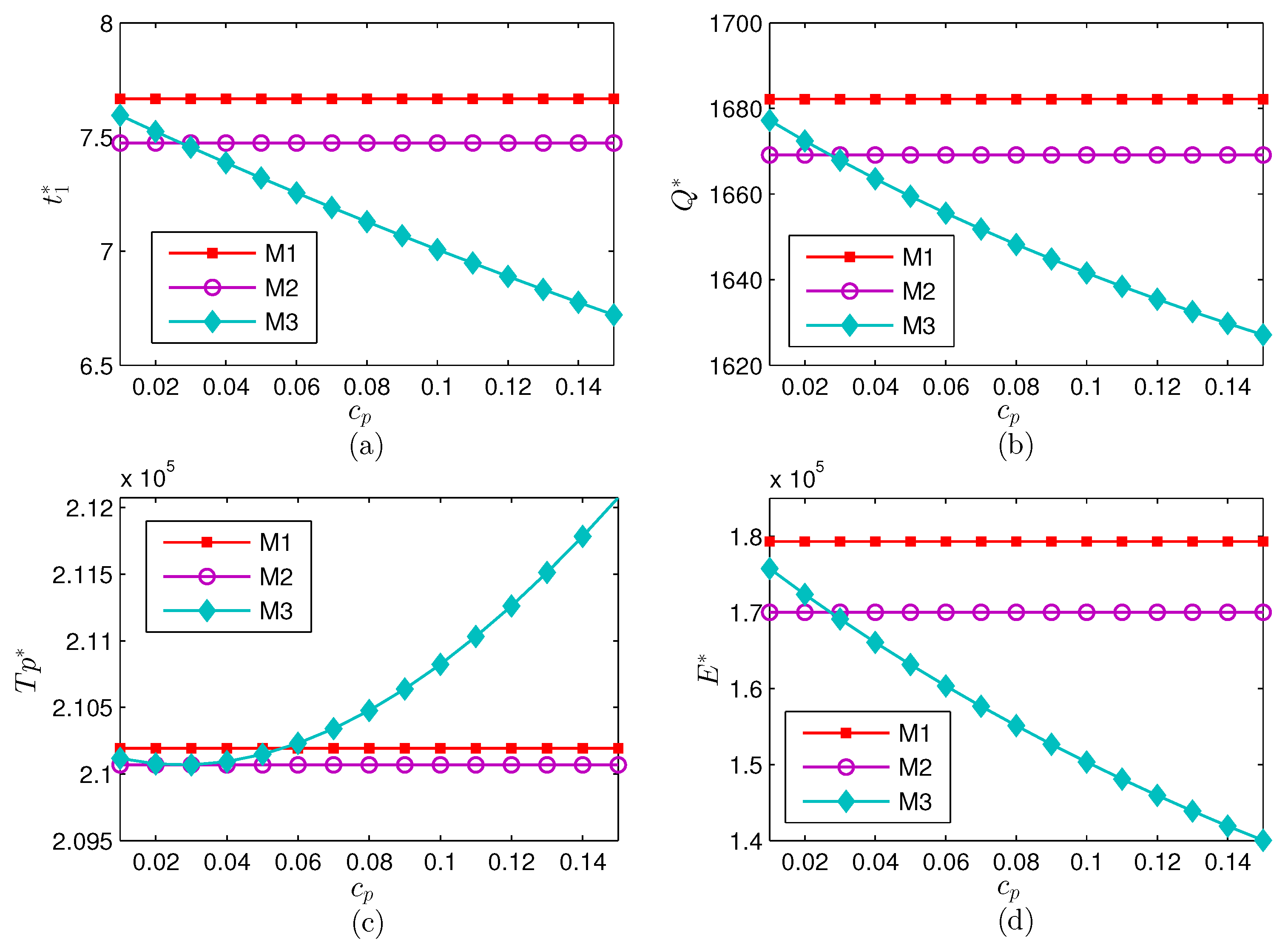
(4) Figure 5 illustrates the impacts of carbon price on the optimal inventory performance. As shown in Figure 5, as carbon price per unit $c_p$ increases, the optimal $t_1^{*}$, $Q^{*}$, and $E^{*}$ for M3 all increase, but the optimal $T{p}^{*}$ decreases first and then increases gradually, which is consistent with Theorem 6(1). That is, when the real carbon emissions of the inventory system exceed the carbon quota set by the government, the optimal total profit decreases with the increase of carbon price. However, once the real carbon emission level is lower than the carbon quota, selling the surplus carbon cap will increase the profit of the system during the period of rising carbon prices in the carbon market.

(5) In addition, from the comprehensive view, Figure 2, Figure 3, Figure 4 and Figure 5 show that the optimal total profit in M3 is always higher than that in M1 or M2, and the optimal carbon emissions in M3 are lower than that in M1 or M2. This implies that, compared with M1 and M2 cases, the M3 case (namely, the cap and trade mechanism) can achieve lower carbon emissions and higher profit performances, which enriches the conclusion of Theorem 6.3 from the perspective of numerical analysis.

8. Sensitivity Analysis and Managerial Insights

To illustrate the application of the model, the robustness of the model and managerial insights will be discussed in this section. As the environment of the inventory system is often dynamic, errors in the model assumptions and parameters usually happen due to the uncertainties in making inventory operation decisions. Thus, it is important for inventory managers to explore the robustness of the model. Here, we examine the impact of errors in estimating model parameters through using the same data in Example 1. The measurements of impacts are $\frac{▵Q_i}{Q_i}$, $\frac{▵E_i}{E_i}$, and $\frac{▵{\Pi }_i}{{\Pi }_i}$, where $▵Q_i=Q_i^{\prime }-Q_i$, $▵E_i=E_i^{\prime }-E_i$, and $▵{\Pi }_i={\Pi }_i^{\prime }-{\Pi }_i$ in the Mi case, $i\in \{1,2,3\}$. $Q_i^{\prime }$, $E_i^{\prime }$, and ${\Pi }_i^{\prime }$ are estimated values of the order quantity, the emissions reduction, and the total profit in the Mi case, and their true values are $Q_i$, $E_i$, and ${\Pi }_i$ respectively.

Table 1. Robustness results of the proposed models.

			M1			M2			M3
Parameters	Chang (%)	$\frac{\mathsf{▵}{\mathit{Q}}_{\mathbf{1}}}{{\mathit{Q}}_{\mathbf{1}}}\mathbf{(}\mathbf{\%}\mathbf{)}$	$\frac{\mathsf{▵}{\mathit{E}}_{\mathbf{1}}}{{\mathit{E}}_{\mathbf{1}}}\mathbf{(}\mathbf{\%}\mathbf{)}$	$\frac{\mathsf{▵}{\mathbf{\Pi }}_{\mathbf{1}}}{{\mathbf{\Pi }}_{\mathbf{1}}}\mathbf{(}\mathbf{\%}\mathbf{)}$	$\frac{\mathsf{▵}{\mathit{Q}}_{\mathbf{2}}}{{\mathit{Q}}_{\mathbf{2}}}\mathbf{(}\mathbf{\%}\mathbf{)}$	$\frac{\mathsf{▵}{\mathit{E}}_{\mathbf{2}}}{{\mathit{E}}_{\mathbf{2}}}\mathbf{(}\mathbf{\%}\mathbf{)}$	$\frac{\mathsf{▵}{\mathbf{\Pi }}_{\mathbf{2}}}{{\mathbf{\Pi }}_{\mathbf{2}}}\mathbf{(}\mathbf{\%}\mathbf{)}$	$\frac{\mathsf{▵}{\mathit{Q}}_{\mathbf{3}}}{{\mathit{Q}}_{\mathbf{3}}}\mathbf{(}\mathbf{\%}\mathbf{)}$	$\frac{\mathsf{▵}{\mathit{E}}_{\mathbf{3}}}{{\mathit{E}}_{\mathbf{3}}}\mathbf{(}\mathbf{\%}\mathbf{)}$	$\frac{\mathsf{▵}{\mathbf{\Pi }}_{\mathbf{3}}}{{\mathbf{\Pi }}_{\mathbf{3}}}\mathbf{(}\mathbf{\%}\mathbf{)}$
$p=60$	$+20$	0.027	0.458	42.489	0	0	42.803	0.034	0.520	42.818
	$+10$	0.014	0.230	21.244	0	0	21.402	0.018	0.262	21.408
	−10	−0.014	−0.235	−21.242	0	0	−21.402	−0.018	−0.265	−21.405
	−20	−0.029	−0.473	−42.483	0	0	−42.803	−0.036	−0.534	−42.807
$c=25$	$+20$	−0.021	−0.352	−17.793	0	0	−17.893	−0.022	−0.319	−17.898
	$+10$	−0.011	−0.177	−8.897	0	0	−8.947	−0.011	−0.160	−8.949
	−10	0.011	0.176	8.898	0	0	8.947	0.011	0.160	8.950
	−20	0.021	0.353	17.797	0	0	17.893	0.021	0.319	17.901
$h=6$	$+20$	−0.193	−3.083	−3.040	0	0	−2.433	−0.163	−2.351	−2.379
	$+10$	−0.098	−1.622	−1.559	0	0	−1.217	−0.083	−1.214	−1.217
	−10	0.102	1.715	1.643	0	0	1.217	0.085	1.296	1.276
	−20	0.209	3.559	3.376	0	0	2.433	0.174	2.683	2.616
$c_1=12$	$+20$	0.006	0.093	−0.034	0	0	−0.063	0.007	0.105	−0.060
	$+10$	0.003	0.046	−0.017	0	0	−0.031	0.003	0.053	−0.029
	−10	−0.003	−0.047	0.017	0	0	0.031	−0.004	−0.053	0.030
	−20	−0.006	−0.093	0.034	0	0	0.063	−0.007	−0.106	0.060
$c_2=8$	$+20$	0.165	2.797	−1.000	0	0	−2.086	0.208	3.232	−1.794
	$+10$	0.088	1.450	−0.534	0	0	−1.054	0.110	1.656	−0.955
	−10	−0.101	−1.639	0.606	0	0	1.043	−0.126	−1.834	1.062
	−20	−0.219	−3.476	1.302	0	0	2.086	−0.271	−3.837	2.263
$K=200$	$+20$	0	0	−0.324	0	0	−0.328	0	0	−0.327
	$+10$	0	0	−0.162	0	0	−0.164	0	0	−0.164
	−10	0	0	0.162	0	0	0.164	0	0	0.164
	−20	0	0	0.324	0	0	0.328	0	0	0.328
${\theta }_0=0.01$	$+20$	0.090	−0.103	−0.117	0.061	0	−0.091	0.057	−0.090	−0.093
	$+10$	0.045	−0.052	−0.059	0.030	0	−0.046	0.028	−0.045	−0.047
	−10	−0.046	0.052	0.059	−0.030	0	0.0457	−0.029	0.046	0.047
	−20	−0.092	0.104	0.118	−0.061	0	0.0916	−0.058	0.091	0.094
$\delta =0.02$	$+20$	−0.058	0.251	−0.116	−0.135	0	−0.180	−0.116	0.188	−0.175
	$+10$	−0.030	0.126	−0.059	−0.068	0	−0.091	−0.059	0.094	−0.088
	−10	0.030	−0.127	0.059	0.069	0	0.091	0.060	−0.095	0.089
	−20	0.062	−0.256	0.120	0.138	0	0.183	0.121	−0.190	0.179
$T=4$	$+20$	5.496	11.275	1.611	4.520	0	−3.638	5.399	10.808	−1.210
	$+10$	2.914	5.535	1.054	2.470	0	−1.133	2.868	5.306	−0.398
	−10	−3.619	−6.348	−1.738	−3.204	0	−0.718	−3.572	−6.053	−0.164
	−20	−7.991	−13.237	−4.343	−7.509	−5.836	−3.311	−7.890	−12.619	−1.069
$\widehat{c}=10$	$+20$	0	13.479	0	−1.241	0	−9.277	−0.004	14.403	−3.580
	$+10$	0	6.314	0	−0.548	0	−3.202	−0.002	6.718	−1.823
	−10	0	−6.740	0	0.455	0	1.0588	0.002	−7.202	1.790
	−20	0	−13.479	0	0.853	−6.099	1.079	0.004	−14.404	3.580
$\widehat{h}=6$	$+20$	0	6.060	0	−0.298	0	−1.479	−0.083	3.592	−1.217
	$+10$	0	2.941	0	−0.158	0	−0.716	−0.042	1.809	−0.620
	−10	0	−3.030	0	0.179	0	0.601	0.042	−1.941	0.631
	−20	0	−6.060	0	0.385	0	0.999	0.085	−3.987	1.276
$\widehat{K}=150$	$+20$	0	0.461	0	−0.034	0	−0.140	0	0.497	−0.123
	$+10$	0	0.230	0	−0.017	0	−0.069	0	0.248	−0.062
	−10	0	−0.230	0	0.017	0	0.066	0	−0.248	0.061
	−20	0	−0.461	0	0.034	0	0.130	0	−0.497	0.123
$c_p=0.5$	$+20$	0	0	0	0	0	0	−0.087	−1.275	0
	$+10$	0	0	0	0	0	0	−0.044	−0.652	−0.008
	−10	0	0	0	0	0	0	0.045	0.670	0.024
	−20	0	0	0	0	0	0	0.089	1.362	0.066
$E=6000$	$+20$	0	0	0	0.524	8.530	1.079	0	0	4.918
	$+10$	0	0	0	0.521	7.860	1.067	0	0	2.400
	−10	0	0	0	−0.790	−10.000	−5.033	0	0	−2.459
	−20	0	0	0	−2.005	−20.000	−18.054	0	0	−4.918

lists the robustness results of the models obtained by varying the value of each inventory parameter while maintaining the same initial values of other parameters. From Table 1, we can reach the following conclusions.

(1) Although deterioration parameter ${\theta }_0$, lost sales coefficient $\delta$, lost sales cost $c_1$, and shortage cost $c_2$ are not easy to be estimated accurately, the effects of these parameters on the order quantity, the emissions reduction, and the total profit are very slight. For instance, in M1, for 20% under or overestimation of ${\theta }_0$, $\frac{▵Q_1}{Q_1}$ changes from −0.092% to 0.09%, $\frac{▵E_1}{E_1}$ changes from 0.104% to −0.103%, and $\frac{▵{\Pi }_1}{{\Pi }_1}$ changes from 0.118% to −0.117%. This shows that estimating errors in ${\theta }_0$, $\delta$, $c_1$, and $c_2$ may not lead to large fluctuations in the optimal solutions. Therefore, the models are robust to the parameters ${\theta }_0$, $\delta$, $c_1$, and $c_2$.

(2) The total profit in the inventory system is more sensitive to the price parameter p and the cost parameter c than other parameters; the order quantity in the inventory system is more sensitive to inventory cycle T than other parameters; and the emission reduction is more sensitive to the parameters T, $\widehat{c}$, and $\widehat{h}$.

(3) It can be observed that K and $\widehat{K}$ have no influence on the optimal solutions of the models, but the total profit in the inventory system is scarcely sensitive to these two parameters. It shows that the impacts of changing K and $\widehat{K}$ on the optimal replenishment policy are very slight.

(4) As discussed above, it can be concluded that the proposed inventory models are basically robust.

From the above discussion on the inventory parameters affecting the inventory performance, the following managerial insights can be obtained.

Considering the high sensitivity of total annual profit to the selling price p and the purchasing cost c, it is recommended that the inventory manager should pay particular attention to the values of those inventory parameters when making inventory decisions. In addition, the emission reduction is more sensitive to the parameters T, $\widehat{c}$, and $\widehat{h}$, but those parameters can be exactly estimated by the actual data from the market. Thus, these parameters will not have much influence on the inventory replenishment policy.

Observing that the order quantity, the emissions reduction, and the total profit are more sensitive to the underestimation of T and E than the overestimation of these two parameters, it is recommended that inventory managers should adopt the optimistic estimation rather than the conservative estimation in evaluating parameters T and E when making decisions in practice.

Noting the utilization of a generalized time-varying factor makes the application scope of the models broader, it is convenient for the decision maker to handle the problems with particular circumstances such as linear demand, time-quadratic demand, exponential demand, and so on.

9. Conclusions and Future Research

In this paper, we develop inventory models with partial backlogging for deteriorating items, and investigate the impacts of carbon emission regulations on the inventory system. In contrast to other related literatures considering environmental regulations, the proposed models impose a general time-varying demand in the system, as the customer demands often change with time in the real deteriorating inventory system. More importantly, under emission regulations, the existence and uniqueness of the optimal solution to each model is discussed and the comparison of optimality among the proposed models is carried out. Numerical examples and robust analysis of the models are presented to illustrate the applicability in practice. Key contributions of this paper include the following.

(1) Under environmental regulations, this article incorporates the deterioration into the inventory system, and the utilization of a generalized time-varying demand makes the application scope of the models broader. For instance, if the demand is set as a specific function (e.g., exponential demand in Example 1 and time-quadratic demand in Example 2), the proposed models can be simplified as the inventory models under certain demand pattern.

(2) Following the above discussion, it can be found that inventory managers can gain more benefits from the cap and trade regulation compared with other cases. Both the theoretical and numerical results show that, under the cap and trade, the quantity of carbon quota does not affect the optimal inventory replenishment policy and the optimal emissions reduction strategy, but the inventory manager can increase the profit performance of the inventory system by selling more carbon emission permits. Furthermore, when the items in the inventory system are higher deteriorating, lower carbon emission reduction can be achieved by lower on-hand inventory level and more shortages, but this will also lead to lower profit. Once lost sales increase in the inventory system, the retailer can adopt a higher on-hand inventory level instead of more shortages. However, this will also lead to higher carbon emissions and higher operation cost of the system.

(3) Following the robust analysis, it can be observed that the impacts of the deterioration, lost sales, and shortages on the optimal solutions are very slight. The total profit in the inventory system is more sensitive to the selling price and cost per unit than other inventory parameters; the order quantity is more sensitive to the inventory cycle than other parameters; and the emission reduction is more sensitive to the inventory cycle, the carbon cap, and the carbon emissions incurred by per unit holding. However, these parameters do not have much influence on the inventory policies, and thus the proposed models are basically robust.

In view of the importance of the inferences for inventory policies and emissions reduction strategies, there are also some limits in this paper. For example, this paper only considers the deterministic inventory issues within a fixed inventory cycle. In the future, more practical situations, such as the stochastic demand and the varying inventory cycle, can be incorporated into the models. In addition, this paper only explore the impacts of the carbon cap policy and the cap-and-trade policy on the inventory system, future study may focus on the low-carbon investment and more carbon regulations like carbon tax, carbon offset policy, and so on.