Thermal Degradation Kinetics and FT-IR Analysis on the Pyrolysis of Pinus pseudostrobus, Pinus leiophylla and Pinus montezumae as Forest Waste in Western Mexico

Abstract

For the first time, a study has been carried out on the pyrolysis of wood residues from Pinus pseudostrobus, Pinus leiophylla and Pinus montezumae, from an area in Western México using TGA analysis to determine the main kinetic parameters (Ea and Z) at different heating rates in a N₂ atmosphere. The samples were heated from 25 °C to 800 °C with six different heating rates 5–30 °C min⁻¹. The Ea, was calculated using different widely known mathematical models such as Friedman, Flynn-Wall-Ozawa and Kissinger-Akahira-Sunose. The Ea value of 126.58, 123.22 and 112.72 kJ/mol (P. pseudostrobus), 146.15, 143.24 and 132.76 kJ/mol (P. leiophylla) and 148.12, 151.8 and 141.25 kJ/mol (P. montezumae) respectively, was found for each method. A variation in Ea with respect to conversion was observed with the three models used, revealing that pyrolysis of pines progresses through more complex, multi-stage kinetics. FT-IR spectroscopy was conducted to determine the functional groups present in the three species of conifers. This research will allow future decisions to be made, and possibly, to carry out this process in a biomass reactor and therefore the production of H₂ for the generation of energy through a fuel cell.

1. Introduction

Around the world, the amount of publications regarding renewable energies and biofuels accounts for a large percentage of the total of approximately 56% [1,2]. In human history, the use of biomass has been required to meet the energy needs. From the 20th century onwards, due to increased energy demand and the excessive use of various fuels, the incorporation of biomass in the fuel mix has been seriously considered, especially in developing countries [3]. Today, biomass is considered one of the main sources of energy, as well as one of the new alternatives that have been implemented to try to reduce the amount of emissions of CO₂, SO_x, NO_x and particulate matter produced during energy production processes [4]. It is worth mentioning that, in the case of CO₂, the use of oil-based fuels, accounts for more than 70% of human related emissions of this gas worldwide, and the rest is attributed to changes in land use. Pollution in some countries is alarming, as is the case in the United States where about 97% of all transport energy is currently derived from oil [5]. Transport energy consumes 63% of all oil used in this country. Because fossil fuels are not renewable and the United States has a need for foreign energy, there is an excellent opportunity to develop renewable energy sources. In this sense, and considering the serious consequences of the greenhouse effect and the future depletion of fossil fuels, there is the possibility of using biomass to produce energy [6]. Given the current scenario in which prosperity is directly related to the capacity to use energy, production resources must be taken into account, especially those that are well distributed in the territory, which are renewable, environmentally appropriate and contribute to reducing CO₂ emissions. Lignocellulosic waste fulfils this purpose [7,8]. It is important to mention that plant biomass is distributed throughout much of the world (except for polar ice caps and extremely dry areas) and grows in different forms (herbaceous plants, shrubs, trees, algae, etc.). In addition, the development of agricultural techniques has considerably increased soil fertility, leading to a greater use of agricultural land for the last 20 to 30 years.

This will allow the generation of energy in certain devices of the latest technology, such as fuel cells, with special emphasis on solid oxides (SOFC), which can generate electricity from the use of gases (H₂, CH₄) from the combustion of biomass or from agricultural waste, industrial and even urban waste (landfills). In this case, the process is produced from obtaining methane gas, pollutant, emitted by organic waste or biomass combustion, which at the time of entering the cell produces electricity. It is important to emphasize that the development of this technology opens in Mexico the access to a wider energy market and includes electricity generation in rural areas, in addition, where the temperature is very low in winter, these systems can work in dual form: heat and power. In winter it would work as a heating and electric power generator, and in summer as an electric generator.

Biomass can be thermally transformed through various thermal processes such as liquefaction, gasification and pyrolysis. Pyrolysis is a well-established route for thermal processing of biomass. The pyrolysis process dates back to the Egyptians, when tar was produced for ship caulking and certain embalming agents [9]. Pyrolysis leads to the conversion of biomass into non-condensable, condensable gases and higher molecular weight compounds such as coal [10]. It is a reality that the lignocellulosic waste pyrolysis process represents a very promising for the near future from the production of various chemical compounds such as bio-oil [11,12]. In thermal processes for the transformation of biomass, pyrolysis is usually the first stage [4]. Currently, there is an extensive bibliography that analyses certain kinetic mechanisms in lignocellulosic biomass. Today, the wood industry is interested in finding a more economical way to dispose of the various waste products from forestry and logging activities. These products, which have been ignored in the past, can now replace oil [13].

Therefore, in order to standardize pyrolytic processes on an industrial scale for the generation of biofuels from these forest residues, the application of modern technologies for obtaining energy carriers and displacing the fuels obtained from fossil materials and consequently the reduction of polluting agents, it is necessary to know in depth what happens in pyrolysis. One of the main aspects to know is the chemical kinetics, because this will be fundamental base for the design of the reaction zone of the process. In the development of pyrolysis, it is necessary to consider the appropriate temperature levels and heating speed. One of the pathways that has gained great diffusion in thermal decomposition analysis of biomass is the study of the decomposition process by thermogravimetric analysis (TGA) [14,15,16]. TGA has been formally defined as a group of techniques in which a property of the sample is controlled against time or temperature, while the temperature of the sample is programmed in a specific atmosphere [17]. The TGA in addition to being applied to plant and animal studies [18], but also for the thermal decomposition of other materials such as medical waste [19], car wrecks [20], PCB waste or sewage sludge [21]. There are also various thermoanalytic techniques classified according to the physical property subject to measurement (see

Table 1. Classification of thermoanalytical techniques [22].

Property	Technique	Parameter Measured	Acronym
Mass.	Thermogravimetric analysis.	Sample mass.	TGA
	Derivative thermogravimetry.	First derivative of mass.	DTG
Temperature.	Differential thermal analysis.	Temperature difference between sample and inert reference material.	DTA
	Derivative differential thermal analysis.	First derivative of DTA curve.
Heat.	Differential scanning calorimetry.	Heat supplied to sample or reference.	DSC
Pressure.	Thermomanometry.	Pressure.
Dimensions.	Thermodilatometry.	Coefficient of linear or volumetric expansion.
Mechanical properties.	Thermomechanical analysis.		TMA
Electrical properties.	Thermoelectrical analysis.	Electrical resistance.	TEA
Magnetic properties.	Thermomagnetic analysis.
Acoustic properties.	Thermoacoustic analysis.	Acoustic waves.	TAA
Optical properties.	Thermoptical analysis.		TOA

).

By using gases such as nitrogen, argon or helium, a TGA analysis can be performed, where the amount of mass lost with respect to a programmed temperature is determined [23]. In this sense and based on various mathematical models, it is possible to obtain very valuable information about the composition of the material, reaction orders, the various stages of thermal transformation, as well as their kinetic behaviour parameters, which is essential in the knowledge of the kinetic behaviour of lignocellulosic materials. This information is basic when designing, building and operating an industrial scale reactor for pyrolysis of the material being studied or for the energetic exploitation of products that can be generated such as hydrogen, for energetic purposes, for example, in fuel cells.

For the determination of the above-mentioned kinetic parameters, non-isothermal methods can be used, which require various heating speeds, although various thermal transformation processes can be affected by changes in the heating rate, thus causing other reactions, which makes analysis by DTG more difficult. [24]. Due to the wide variation in the parameters of the Arrhenius equation [25], today, there are several mathematical models for calculating Arrhenius variables. These so-called “model-free” methods are based on an iso-conversive basis, where an assumption is made that the rate of progression of a reaction is constant and therefore the speed of the reaction depends only on the temperature of the reaction. Considering the activation energy (Ea) as the main variable, iso-conversion methods do not require prior knowledge of the reaction mechanism in thermal conversion of the biomass under study, i.e., it is not necessary to choose a reaction model [26]. Non-isothermal iso-conversional methods can follow a differential approach such as Friedman [27], and non-differential (integral) methods Flynn-Wall-Ozawa (FWO) [28] and Kissinger-Akahira-Sunose (KAS) [29,30]. Considering an attractive alternative to oil, with a zero impact of CO₂, its energy capacity and amount of waste approximately 1300 m³/year (sawdust and shavings) of Pinus pseudostrobus, Pinus leiophylla and Pinus Montezumae as the most commercial and important forest species of the industrial-wood locality of San Juan Nuevo Parangaricutiro (Purépecha zone of the state of Michoacán, Mexico); the aim of this research and for the first time, the mathematical models of Friedman, FWO and KAS are used to determine the most important variables of the kinetic process (Ea and Z)in the inert atmosphere of the thermal degradation of the three selected species of pine. It is important to mention that no articles have been found that refer to the kinetic analysis of the thermogravimetric process for these forests’ species pine.

On the other hand, that despite the fact that in recent years the main components of lignocellulosic materials have been analysed through infrared spectroscopy (IR), it is necessary to study their primary composition in greater depth. Today, the analysis of the main components of plant biomass such as cellulose, hemicellulose, lignin and other polymers is well studied and their chemical changes with infrared spectroscopy through Fourier Transform Infrared (FT-IR). In addition to kinetic analysis, in this paper, the results of FT-IR are presented to the three species of pine.

2. Methods

2.1. Sample Preparation and Chemical Composition Analysis

Random samples, of known origin, were taken from different workshops of San Juan Nuevo Parangaricutiro, Michoacán, Mexico, taking precautions to avoid contamination with other types of wood and other substances such as solvents, ensuring that only P. pseudostrobus, P. leiophylla and P. Montezumae waste represented each sample. Pyrolysis is the term commonly used for a high temperature treatment. The analysis of this type of treatment should include: drying, devolatilization and mainly in the events that occur in the formation of coal, which is one of the main objectives of this article. Each of the samples were placed in containers in a dry place at room temperature (25 °C) for 2 days to eliminate the superficial humidity with which the sample arrives. Afterwards, the fine grain milling was carried out. Once dried, a sieve was made in order to obtain samples with a particle size of approximately 200 µm. Finally, the biomass was taken to an oven to dry at 115°C monitoring until a constant weight was obtained.

In previous investigations, the chemical composition of P. pseudostrobus, P. leiophylla and P. Montezumae, located in the aforementioned area of Michoacán state has already been determined [31]. In this case, the ash analysis was carried out on an X-ray spectrometer, coupled to a SEM (Jeol JSM-6400) [32]. The minerals were calculated (UNE-EN 14775) [33]. It should be noted that due to the high volume (1300 m³/year) of waste produced and the energy potential it represents for the community in question, research of these woods has continued.

2.2. Thermogravimetric Analysis TGA-DTG

A Simultaneous Thermal Analyzer STA 6000 thermogravimetric analyzer (PerkinElmer, city, state abbrev if USA, country) was taken after sample preparation and with a uniform particle size to perform a gradual mass degradation at different heating rates (β = 5–30 °C/min). The non-isothermal model was carried out with each heating rate β (six analyses), from 25 °C to 120 °C, left in isotherm for 12 min and then the system was brought to a temperature of 800 °C at the same heating rate to continue with one more isotherm for 30 min, then cooling to room temperature. In the thermobalance of the TGA equipment, a ceramic crucible was used where between 6.5 and 7.5 mg were placed of sample, in order to reduce the effects of mass transfer and heat transfer, because the presence of temperature gradients in the bed of the material and the particles cause that the biomass does not react homogeneously and there are differences in the sequence of reactions, due to the conditions of transport of the primary products of the reactions to the outside of the particles and through the bed of the material. These transport processes are largely responsible for the secondary reactions, which are generated from the primary products of biomass pyrolysis [4]. All thermal degradations were carried out in an inert atmosphere of high purity (99.99%) nitrogen (N₂) as reaction gas with a flow rate of 50 mL/min. Before each experiment, N₂ was purged for 45 min at a flow rate of 100 mL/min.

2.3. Kinetic Modeling

The kinetics of free models are based on iso-conversion methods and are mainly used for obtaining and evaluating the activation energy, which is a function of the degree of conversion of a chemical reaction. Such methods are widely recommended [34]. Because thermographs, TGA results, contain partially superimposed peaks, mathematical models are generally used for deconvolution [35]. It has been proven that the values obtained depend not only on factors such as atmosphere, gas flow, sample mass and heating rate, but also on the mathematical treatment of the data. To evaluate such data at different heating rates, this paper describes the pyrolysis process from three iso-conversional kinetic models, one differential corresponding to Friedman [26], and two integrals, one from Flynn-Wall-Ozawa (FWO) [36] and the other from Kissinger-Akahira-Sunose (KAS) [28]. With these methods, the kinetic parameters that characterize the thermal degradation process of biomass can be obtained. The data from the TGA curves were used to determine the kinetic parameters.

The general process of pyrolysis of biomass can be represented as [37]:

The overall kinetics of the biomass pyrolysis reaction can be described as follows:

$$\frac{d\alpha }{dt}=k\left(T\right)f\left(\alpha \right)$$

(1)

Practically all the proposed kinetic models employ a law that obeys Arrhenius fundamental velocity expression, so Equation (1) can be expressed as:

$$\frac{d\alpha }{dt}=\frac{A}{\beta }exp\left(-\frac{E_a}{RT}\right)f\left(\alpha \right)$$

(2)

where f(α) is a conversion function which, as can be seen in

Table 2. Functions of the most common reaction mechanisms for gas solid reactions [34].

Symbol	Mechanism	g(α)	f(α)
D1	Diffusion One-way transport	α2	1/2α
D2	Two-way transport	α + (1 − α)ln(1 − α)	[− ln(1 − α)]−1
D3	Three-way transport	[1 − (1 − α)1/3]2	(3/2)(1 − α)2/3[1 − (1 − α)1/3]−1
G-B	Ginstling-Brounshtein equation	1 − (2/3)α − (1 − α)2/3	(3/2)[(1 − α) − 1/3 − 1]−1
Zh	Zhuravlev equation	[(1 − α)−1/3 − 1]2	(3/2)(1 − α)4/3[(1 − α)−1/3 − 1]−1
A2	Random nucleation and nuclei growth Bi-dimensional	[−ln(1 − α)]1/2	2(1 − α)[−ln(1 − α)]1/2
A3	Tree-dimensional	[−ln(1 − α)]1/3	3(1 − α)[−ln(1 − α)]2/3
P-T1	Prout-Tompkins (m = 0.5)	ln[(1 + α1/2)/(1 − α1/2)]	(1 − α) α1/2
P-T2	Prout-Tompkins (m = 1)	ln(α/(1 − α)]	(1 − α) α
F1	Chemical reaction First-order	−ln(1 − α)	1 − α
F2	Second-order	(1 − α)−1 − 1	(1 − α)2
R1	Limiting surface reaction between both phase One dimension.	α	1
R2	Two dimension	1 − (1 − α)1/2	2(1 − α)1/2
R3	Three dimension	1 − (1 − α)1/3	3(1 − α)2/3

, represents the reaction model used and depends on the control mechanism [38,39,40]; dα/dt is the speed of the isothermal process; T is the absolute temperature (K), α is the degree of conversion, A is the pre-exponential factor or frequency factor (min⁻¹), which is the frequency of molecular collisions, regardless of their energy level [41]. Ea, (activation energy) is the maximum energy required in a reaction to form a certain amount of products [42], R is the universal gas constant equal to 8.314 J/(mol K) and β is the linear heating velocity (β = dT/dt) and it’s a constant. The exponential term of Equation (2) can be considered as the fraction of collisions that has sufficient kinetic energy to induce a reaction, thus the product Aexp^−Ea/RT produces the frequency of collisions that are successful [43]. It is important to mention that derived from the exponential term of the Arrhenius equation, there is a dependence on temperature, it should also be noted that the variable A (pre-exponential factor) also depends on temperature behavior [44]. The degree of conversion (α) or also called process coefficient, can be defined as the mass fraction that has been decomposed or the mass fraction of volatile compounds and is expressed as α = (m₀ − m)/(m₀ − m_∞) where m is the mass of substrate present at any time t, m₀ is the initial mass of the substrate and m_∞ is the final mass of solids (unreacted residue) that remains after the reaction.

The analysis of the thermal degradation of biomass is carried out with the application of a series of diverse kinetic models, which can be applied to its degradation process in addition to the dynamic analyses of thermal degradation. In this sense, iso-conversion methods assume a fixed value of α, thus only the temperature is a decisive factor for the speed of reaction. Thus, it is possible to calculate the Ea, considering α, independently of the reaction model f(α). Iso-conversion methods can be differential or integral for the treatment of differential thermal analysis data.

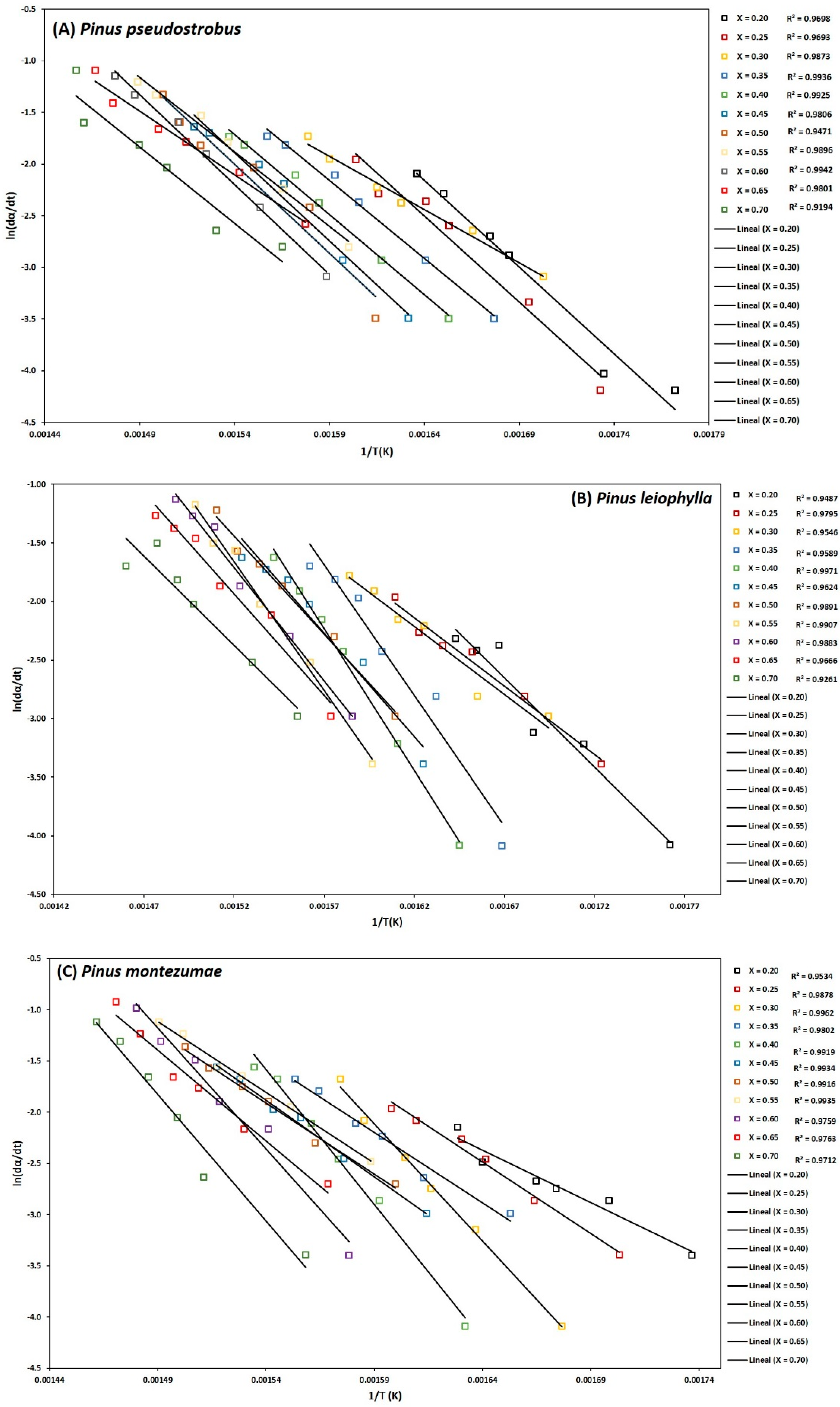
2.3.1. Friedman Method

In the case of iso-conversional differential models, Friedman’s method is probably the most general of the derived techniques. It is based on the comparison of the conversion velocity dα/dT for a conversion grade α determined, using different heating rates [45]. It is necessary to work with a degree of advance range α in which the linear fit is adequate. Considering the natural logarithm on both sides of Equation (2) and simplifying, the general equation of this method is as follows:

$$ln\left(\frac{d\alpha }{dt}\right)=ln\left[\beta \left(\frac{d\alpha }{dT}\right)\right]=ln\left[Af\left(\alpha \right)\right]-\frac{Ea}{RT}$$

(3)

By analogy of the general equation of the straight line (y = mx + b), through the Friedman method, it is possible to obtain the value of the activation energy by graphing ln(dα/dt) vs. 1/T, for each conversion value, α, at different heating rates. The resulting graph will show several lines that, according to Equation (3), will have a slope (m) equal to −Ea/R [46].

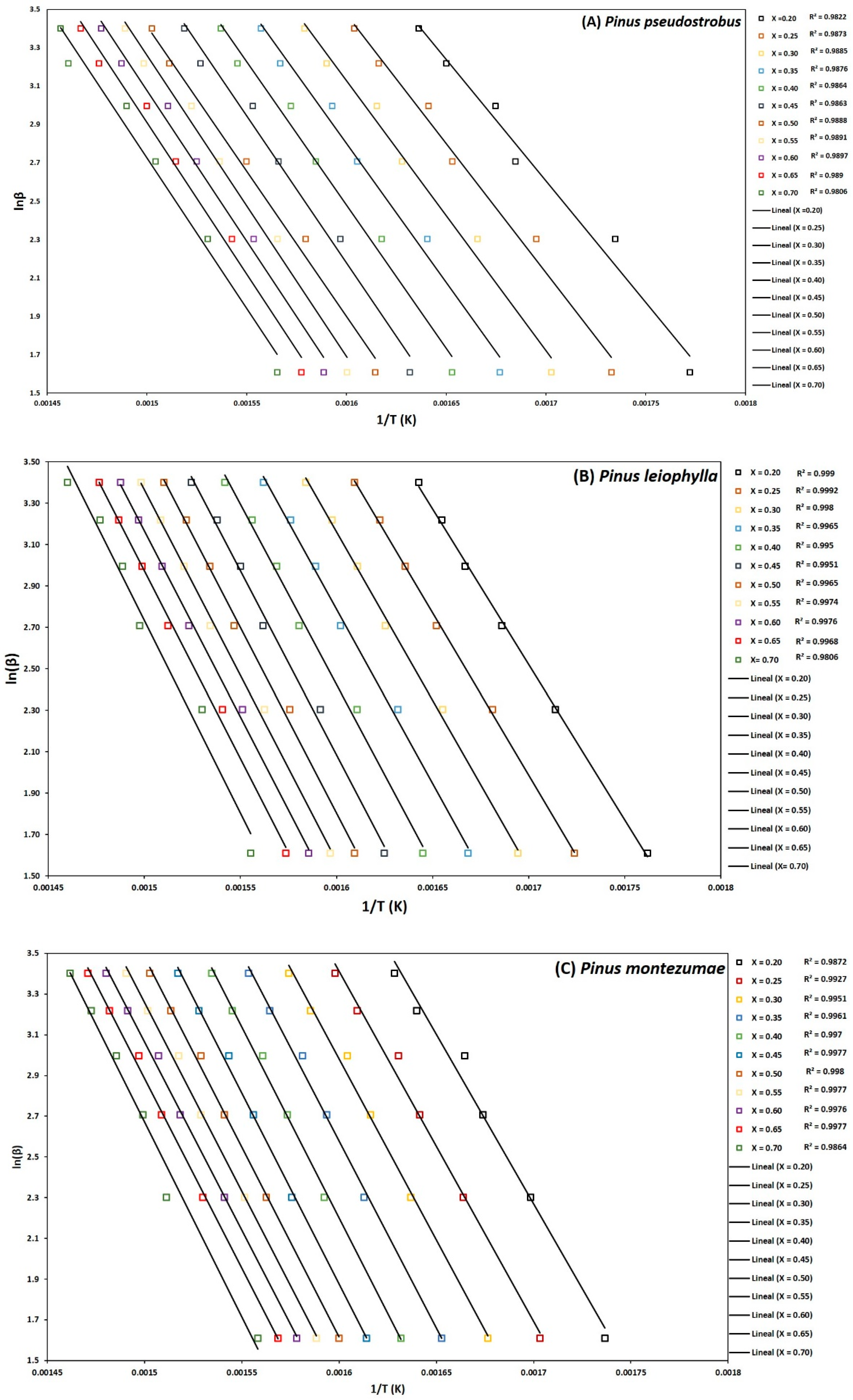
2.3.2. Flynn-Wall-Ozawa Method (FWO)

The FWO method is one of the most common and widely accepted methods in the scientific community for calculating thermokinetic parameters from experimental data. This method uses a correlation between the heating rate of the sample, the activation energy and the temperature inverse [47]. It is an integral and iso-conversional technique that assumes that Ea is constant in every reaction process considering time from t = 0 until t_∞, where t_∞ is the conversion time of α [48].

Integrating Equation (3) with respect to the variables α and T results:

$$g\left(\alpha \right)={\int }_0^{\alpha }\frac{d\alpha }{f\left(\alpha \right)}=\frac{A}{\beta }{\int }_0^{T_{\alpha }}exp\left(\frac{-Ea}{RT}\right)dT$$

(4)

where T_∞ is equal to the conversion temperature α. Considering the value of Ea/RT equal to x, Equation (4) is transformed into:

$$g\left(\alpha \right)=\frac{A{E}_a}{\beta R}{\int }_{\alpha }^{\infty }\frac{ex{p}^{-x}}{x^2}=\frac{A{E}_a}{\beta R}p\left(x\right)$$

(5)

where p(x) represents the integrand on the right side of Equation (4) and is known as the temperature integral. This integral does not have an exact analytical solution [49], however, as noted below, it can be approximated through an empirical interpolation formula proposed by Doyle [50]:

log p(x) ≅ −2.315 − 0.4567x, for a range x: 20 ≤ x ≥ 60

(6)

Considering this approximation to the right member of Equation (4) and applying the natural logarithm on both sides of the equation the final form of the OFW model is obtained:

$$log\beta =log\left(A\frac{E_a}{Rg\left(\alpha \right)}\right)-2.315-0.4567\frac{Ea}{RT}$$

(7)

According to Equation (7) and when graphing the logβ versus 1/T at different heating rates, parallel straight lines are obtained for each degree of conversion α. The value of the apparent activation energy is calculated across the slope of those lines. Such slope is proportional to the expression −0.4567E_a/R. The value of logA is given by the intercept (logβ) of each line with the vertical axis of the graph.

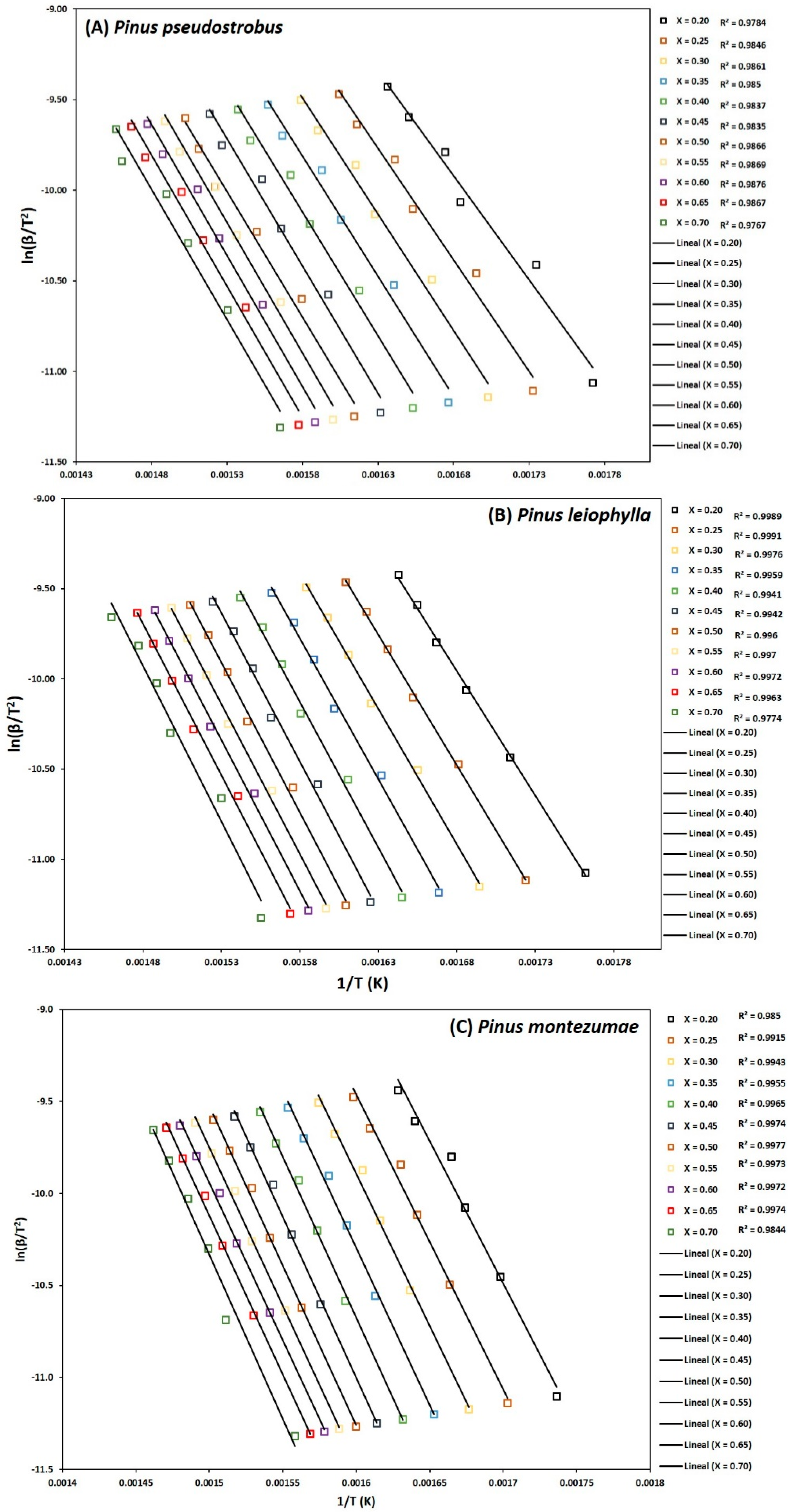
2.3.3. Kissinger-Akahira-Sunose Method (KAS)

The KAS method is a non-isothermal iso-conversional technique which, like the previous method, is widely used. The KAS method uses the Arrhenius equation using a differential method. This method does not require knowledge of the exact thermal degradation mechanism [51]. The KAS method is derived from Equation (2), which is integrated from specific conditions (x = 0, T = T₀), to get the following expression:

$$g\left(x\right){\int }_0^x\frac{dx}{f\left(x\right)}=\frac{A}{B}{\int }_{T_o}^{T}exp\left(-\frac{E}{RT}\right)dT\equiv \frac{AE}{\beta R}p\left(\frac{E}{RT}\right)$$

(8)

As can be seen from Equation (8), the frequency factor A, the function f(x) and the activation energy Ea, are temperature-dependent T, however Ea and A are independent of x. By re-integrating Equation (8), an expression is obtained as a function of natural logarithms:

$$ln \left(g\left(\alpha \right)\right)=ln\left(\frac{AE}{R}\right)-ln\beta +ln \left(p\frac{E}{RT}\right)$$

(9)

Considering the approximation of Coats-Redfern [52] where:

$$p\left(\frac{E_a}{RT}\right)\cong \left[\frac{exp\left(-\frac{E_a}{RT}\right)}{{\left(\frac{E_a}{RT}\right)}^2}\right]$$

(10)

Combining Equations (9) and (10) and simplifying gives the main expression of the KAS method:

$$ln\frac{\beta }{T^2}=ln\left[\frac{AR}{E_{a}g\left(\alpha \right)}\right]-\frac{E_a}{RT}$$

(11)

From Equation (11) the apparent activation energy can be obtained by graphing ln(β/T²) versus 1/T where the value of the slope of the line obtained is equal to −Ea/R for a constant value of the degree of conversion, α.

2.3.4. Frequency Factor (Z)

Because the vast majority of thermal analyses are carried out at a constant heating rate, a more useful approach for the Arrhenius integral has been implemented under experimental conditions of a linear temperature program and to extend these results of the unequivocal determination of the Arrhenius kinetic parameters by establishing the iso-conversional method whose final expression is [53]:

$$Z=\frac{\beta \ast \left(E_a+2\ast R\ast T_{\alpha }\right)\ast e^{\frac{E_a}{R{T}_{\alpha }}}}{R\ast T_{\alpha }^2}$$

(12)

where: Z, is the frequency factor (min⁻¹), β, is the heating speed (°C/min), Ea, is the activation energy (kJ/mol), Tα is the temperature (K), where the maximum conversion is reached (α).

2.4. Fourier Transform Infrared Analysis (FT-IR)

The infrared spectroscopy technique will identify the main gaseous products produced during the pyrolysis of the three forest species. The The FT-IR values of the lignocellulosic materials were obtained using the PerkinElmer ATR 400 model resolution 4 cm⁻¹. The biomass was prepared with methods well established in the literature for IR analysis. All the spectra were acquired (16 scans/sample) in the range of 650–4000 cm⁻¹ with 4 cm⁻¹ resolution.

3. Results and Discussion

3.1. Chemical Analysis

Table 3. Chemical analysis of P. pseudostrobus, P. leiophylla and P. montezumae wood sawdust [27].

Parameter	P. pseudostrobus	P. leiophylla	P. montezumae
Ash (%)	0.19 (±0.1)	0.23 (±0.06)	0.13 (±0.01)
Elemental ash composition of forest residues the three conifers (%)
Ca	25.48 (±0.5)	42.46 (±0.98)	42.44 (±0.54)
K	12.23 (±0.77)	13.16 (±0.78)	21.1 (±0.66)
Mg	10.82 (±0.44)	21.64 (±0.31)	13.08 (±0.47)
P	9.35 (±0.54)	5.37 (±0.20)	4.06 (±0.16)
S	1.70 (±0.21)	3.8 (±0.18)	2.59 (±0.09)
Na	2.17 (±0.37)	5.74 (±0.61)	2.33 (±0.29)
Si	17.46 (±0.70)	4.57 (±0.43)	4.89 (±0.61)
Al	12.70 (±0.69)	3.22 (±0.51)	6.26 (±0.28)
Fe	7.01 (±0.33)	no detected	3.21 (±0.24)
Ti	0.5 (±0.1)	no detected	no detected

shows the results of the elementary analysis of P. pseudostrobus, P. leiophylla and P. montezumae previously obtained by some of the authors who collaborated in this research [30]. A low ash content (0.13–0.23%) can be observed in all three species of pine, which is very significant and attractive in the thermal degradation processes of lignocellulosic biomass [22]. A high degree of ash in the fuel can damage combustion equipment and users when they have to do cleaning work [54]. With regard to the mineral composition of the ash, the elements, calcium, potassium, magnesium, silicon and aluminium, were the elements that were presented in greater quantity. It should be noted that the content of potassium (12.23–21.1%) and sodium (2.17–5.74%), help reduce the melting point of the ash [55,56]. A high content of magnesium (Mg), allows an increase in the melting point of the ash. It should also be mentioned that the high amount of calcium (25.48–42.46%) reduces the amount of ash, although it can increase its melting point [22]. Silicon, is fixed in silicates. In this case the amount of silicon (4.57–17.46%) helps to significantly reduce the melting point of the ash [57].

3.2. Thermogravimetric Analysis

Figure 1A–C, illustrate the P. Pseudostrobus, P. leiophylla and P. montezumae curves with respect to mass loss and temperature (TGA) for heating rates of 5, 10, 15, 20, 25 and 30 °C/min in nitrogen inert atmosphere. The curves show the typical appearance of pyrolysis of lignocellulosic materials and from them the thermal phases for each of the β can be located. The main reactions consist of broken glycosidic bonds with the consequent partial depolymerization of the cellulosic component of the wood.

According to several researchers, hemicellulose decomposes in a range between 180–340 °C, which is less than cellulose when decomposing between 230–450 °C and the latter less than lignin, which is thermally transformed at a temperature greater than 500 °C [53,58]. Cellulose decomposition occurs in two ways. First, the bonds are divided into monomers at a lower temperature and form CO, CO₂ and carbonaceous gases. Then, at a higher temperature, liquid formation occurs. In stage three, lignin decomposes at a temperature above 500 °C and at a slower rate due to an association with a hydroxyl phenolic group. At this stage there is the presence of high molecular weight carbonaceous products.

The thermograms of Figure 1A–C, can be divided into four distinct zones, zone 1 (T < 50 °C), which corresponds to an increase in mass which is attributable to condensation of water and the formation of intermediate compounds which are subsequently decomposed. Zone 2 (T ≈ 135 °C), where moisture evaporation takes place and the release of CO, CO₂, and extractable materials. According to the literature, between 180 and 400 °C the highest devolatilization occurs, which has been designated as the zone of active pyrolysis [59]. At a temperature higher than 200 °C and up to approximately 400 °C, zone 3 is present, where the maximum degradation of hemicellulose, cellulose and lignin is reached about 80% of the total mass. During this stage most of the volatiles were released and the evolution of the secondary gases was practically completed at 400 °C, which led to the formation of carbon [60]. In the passive zone, there is no decomposition but the carbon and ashes are part of the final solid waste. It is worth mentioning that from 400 to 700 °C the condensed system grows gradually, but all peripheral atoms are bonded by chemical bonds to hydrogen atoms or hydrocarbon groups, substances that have high electrical resistivity. It is important to mention that high heat flows in the highest heating zone decrease the viscosity level in the material, while increasing the reactions that form the volatiles. This behavior has been previously described for several biofuels [61,62]. The highest mass loss is identified at the maximum peak in the thermo-differential analysis (DTG) curves. DTG is shown in Figure 2A–C. As predicted, the graphs show three main areas. First peak is observed due to the elimination of moisture and light volatile matter when heated from 50 to approximately 135 °C. The main stage of thermal decomposition is carried out in a temperature range between 200–400 °C at heating rates between 5–30 °C/min. Two peaks are observed that are evidence of hemicellulose and cellulose decomposition, while there is no indication of any peak derived from lignin decomposition [63]. The second (280–340 °C) and third peak (350–400 °C) appear when hemicellulose and cellulose compounds are transformed. In the final part, the lignin has been transformed at a lower speed, so that a maximum carbonization has been carried out. A comparison between the peaks of hemicellulose, cellulose and lignin shows that they have different height and position, which indicates the influence of the distribution of organic and inorganic compounds in the thermal degradation process of P. pseudostrobus, P. leiophylla and P. montezumae.

It is observed that as the heating rate increases, so does the temperature at the beginning and end of pyrolysis. The region where the moisture is volatilized does not show a greater variation with the change of the heating rate. Another important aspect is that the maximum points of the TGA curves and the minimum points of the DTG curves move towards higher temperatures. This is related to the heat transfer concept, where at a lower heating rate, there is locally greater thermal energy, which promotes that the balance with the inert atmosphere takes longer. In parallel, and in the same heating range, there is an increase in the heating rate which promotes a decomposition of the sample at a higher temperature, causing the curve in this heating zone to move in a rightward direction [64]. This phenomenon has also been observed by other researchers [65,66].

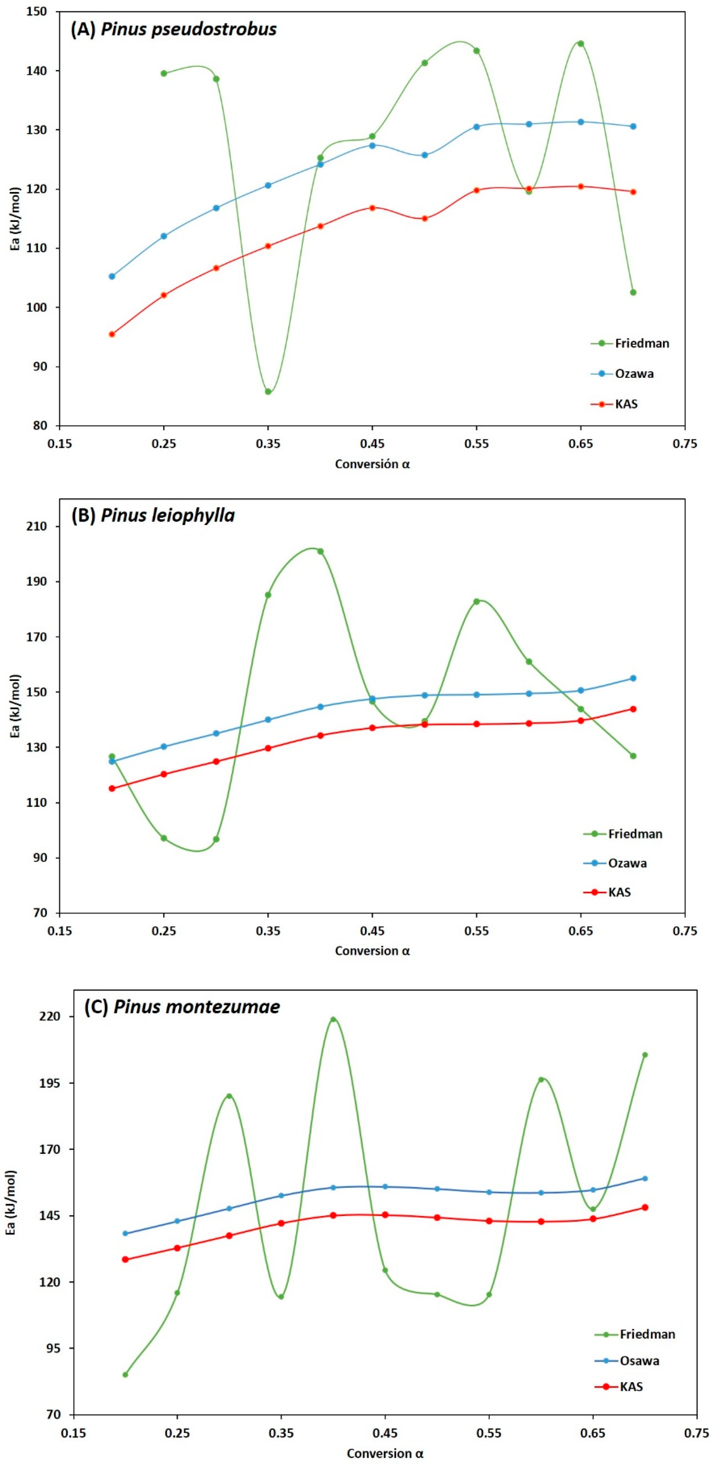
3.3. Kinetic Analysis

The kinetic parameters have been studied in a distributed manner according to the possible values by careful sampling. The distribution of the kinetic parameters is reported for each model used. From the data obtained from the thermogravimetric analysis and for a given fractional conversion value (α), the three iso-conversional kinetic methods mentioned above from Friedman, FWO and KAS were used to determine the values of the main kinetic parameters such as activation energy (Ea) and frequency factor (Z) for each value from α, during pyrolysis of the P. pseudostrobus, P. leiophylla and P. montezumae. Equations (3), (7) and (11) were used for each method. Figure 3A–C, shows the conversion change, α, with respect to temperature at different heating rates for each pine species and it can be seen that activation energy is a function of fractional conversion, this is because most lignocellulosic biomass pyrolysis reactions do not represent a single-step global mechanism, on the contrary, it follows a multi-stage reaction, which means that pyrolysis of P. pseudostrobus, P. leiophylla and P. montezumae, is a complex process consisting of several reactions.

To determine the kinetic parameters, values have been selected from α where the calculated squares of the correlation coefficient, R², were greater than 0.90 for all curves at different heating rates and locating the corresponding temperature. The graphs of the Friedman methods, ln[dα/dt] versus 1/T; Flynn-Wall-Ozawa (FWO), lnβ versus 1/T; and Kissinger-Akahira-Sunose (KAS), ln(β/T²) versus 1/T, for different conversion values, α, are shown in Figure 4A–C, Figure 5A–C, and Figure 6A–C, for P. pseudostrobus, P. leiophylla and P. montezumae, respectively. The apparent activation energies, Ea, were obtained from the slopes in each model (see

Table 4. Ea (kJ/mol) and R² for P. pseudostrobus, P. leiophylla and P. montezumae by Friedman, FWO and KAS methods, R² corresponding to linear fittings in Figure 4A–C, Figure 5A–C and Figure 6A–C.

	Conversion (α)	Ea, Friedman	R2	Ea, FWO	R2	Ea, KAS	R2
	0.20	139.60	0.9698	105.24	0.9822	95.48	0.9784
	0.25	138.62	0.9693	112.02	0.9873	102.04	0.9846
	0.30	85.72	0.9873	116.79	0.9885	106.65	0.9861
	0.35	125.29	0.9936	120.66	0.9876	110.36	0.985
PP	0.40	128.95	0.9925	124.18	0.9864	113.75	0.9837
	0.45	141.33	0.9806	127.37	0.9863	116.80	0.9835
	0.50	143.34	0.9471	125.76	0.9888	115.082	0.9866
	0.55	119.56	0.9896	130.52	0.9891	119.75	0.9869
	0.60	144.58	0.9942	130.97	0.9897	120.11	0.9876
	0.65	102.50	0.9801	131.34	0.989	120.41	0.9867
	0.70	122.88	0.9194	130.58	0.9806	119.55	0.9767
	Average	126.58	0.9748	123.22	0.9868	112.72	0.9841
	0.20	126.63	0.9487	124.86	0.9990	115.09	0.9989
	0.25	97.06	0.9795	130.28	0.9992	120.31	0.9991
	0.30	96.81	0.9546	135.02	0.9980	124.88	0.9976
	0.35	185.14	0.9589	139.99	0.9965	129.70	0.9959
PL	0.40	201.07	0.9971	144.75	0.9950	134.32	0.9941
	0.45	146.74	0.9624	147.59	0.9951	137.03	0.9942
	0.50	139.45	0.9891	148.89	0.9965	138.23	0.9960
	0.55	182.75	0.9907	149.14	0.9974	138.40	0.9970
	0.60	161.10	0.9883	149.53	0.9976	138.71	0.9972
	0.65	143.94	0.9666	150.64	0.9968	139.73	0.9963
	0.70	126.93	0.9261	154.96	0.9806	143.94	0.9774
	Average	146.15	0.9692	143.24	0.9956	132.76	0.9948
	0.20	85.16	0.9534	138.33	0.9872	128.45	0.9850
	0.25	115.97	0.9878	142.98	0.9927	132.89	0.9915
	0.30	190.20	0.9962	147.80	0.9951	137.57	0.9943
	0.35	114.47	0.9802	152.57	0.9961	142.19	0.9955
PM	0.40	218.99	0.9919	155.63	0.9970	145.12	0.9965
	0.45	124.45	0.9934	155.93	0.9977	145.31	0.9974
	0.50	115.32	0.9916	155.09	0.9980	144.38	0.9977
	0.55	115.27	0.9935	153.93	0.9977	143.12	0.9973
	0.60	196.31	0.9759	153.69	0.9976	142.81	0.9972
	0.65	147.50	0.9763	154.74	0.9977	143.79	0.9974
	0.70	205.71	0.9712	159.129	0.9864	148.12	0.9844
	Average	148.12	0.9828	151.80	0.9948	141.25	0.9940

PP: Pinus pseudostrobus; PL: Pinus leiophylla; PM: Pinus montezumae.

) and the average frequency factors from Equation (12), which can be seen in

Table 5. Average frequency factor Z (s⁻¹) calculation results as a function of α (0.70 ≤ α ≥ 0.20) and β (°C/min) for Pinus pseudostrobus, Pinus leiophylla and Pinus montezumae obtained by Friedman, FWO and KAS kinetic models.

		β	5	10	15	20	25	30
PP	FRIEDMAN	Z	6.28 × 109	6.48 × 109	4.46 × 109	4.73 × 109	3.87 × 109	3.72 × 109
	OFW		1.69 × 108	1.89 × 108	1.71 × 108	1.79 × 108	1.50 × 108	1.55 × 108
	KAS		1.95 × 107	2.29 × 107	2.15 × 107	2.30 × 107	1.98 × 107	2.08 × 107
PL	FRIEDMAN	Z	1.06 × 1014	8.90 × 1013	6.24 × 1013	6.16 × 1013	5.62 × 1013	4.71 × 1013
	OFW		9.04 × 109	9.66 × 109	8.24 × 109	8.69 × 109	8.62 × 109	8.10 × 109
	KAS		1.07 × 109	1.19 × 109	1.06 × 109	1.13 × 109	1.14 × 109	1.09 × 109
PM	FRIEDMAN	Z	2.65 × 1015	1.78 × 1015	1.59 × 1015	1.50 × 1015	1.22 × 1015	1.09 × 1015
	OFW		3.88 × 1010	3.58 × 1010	3.64 × 1010	3.82 × 1010	3.45 × 1010	3.34 × 1010
	KAS		4.61 × 109	4.47 × 109	4.66 × 109	4.97 × 109	4.59 × 109	4.50 × 109

PP: Pinus pseudostrobus; PL: Pinus leiophylla; PM: Pinus montezumae. OFW: Flynn-Wall-Ozawa; KAS: Kissinger-Akahira-Sunose.

.

The Friedman, OFW and KAS models adjust to the degradation of P. pseudostrobus, P. leiophylla and P. montezumae since the correlation coefficient, R², is close to 1 in the conversion range (α) of 0.20, 0.25, 0.30, 0.35, 0.40, 0.45, 0.50, 0.55, 0.60, 0.65 and 0.70. It is important to mention that, using the available experimental data and during the adjustment of the data in each model, low correlation was observed for conversion values lower than 0.20 and higher than 0.70, which means that the R² values showed a low correlation value [34,67]. Iso-conversional methods (model-free) allow to estimate the activation energy as a conversion function without a previous assumption in the reaction model and allow to detect almost unequivocally the kinetics of multiple steps as a dependence of the activation energy (Ea) with respect to the conversion (α), in contrast to methods like Kissinger’s, which produces a single Ea value for the whole process and the complexity of the system may not be accurately revealed [68].

The average of the activation energies (Table 4) calculated from the Friedman, OFW and KAS methods was 126.58, 123.22 and 112.72 kJ/mol respectively with regard to P. pseudostrobus; 146.15, 143.24 and 132.76 kJ/mol respectively for P. leiophylla and 148.12, 151.80 and 141.25 kJ/mol respectively for P. montezumae, checking the compatibility of the data obtained in the thermal transformation of biomass by TGA, being compatible with the proposed mathematical models when conversion values between 0.20 and 0.70 are used.

Similar results have been reported in other kinetic studies of thermal processes in forest residues for several pine species. For example, Pinus insignis, a change in Ea energy in the range of 62–206 kJ/mol was found [69]. Da silva et al., reported the kinetic mechanism of Pinus elliottii and calculated an average Ea of 145.24 kJ/mol [10]. Domínguez et al. reported Ea values for pyrolysis of Pinus radiata residues in the range of 117.7–135.5 kJ/mol [70]. As can be seen there are some differences in the Ea values obtained in this investigation, however, it should be noted that the results for the apparent activation energy reflect contributions from various stages where reactions occur that contribute to changing the speed of the overall reaction process. The previous behaviour, in processes of thermal transformation of lignocellulosic materials, presents variations both in temperature and in the reaction level or degree of reaction, frequently observing an overlapping of such parameters [71,72]. On the other hand, the activation energy depends on the pyrolysis reaction mechanism. As mentioned above, the Ea is the minimum required to carry out an alteration in the bonds of each atom involved in the reaction, therefore as the activation energy is higher, the speed of the reaction will be lower. Generally, variables such as the degree of speed of the entire reaction, as well as the system’s reaction level, will be governed by this parameter.

Several authors state that the reactivity of fuels derived from the pyrolysis of biomass can be calculated from the calculated activation energy of a thermal process [73]. Fuel reactivity is of great importance when planning the design and development of a pyrolytic reactor for lignocellulosic biomass. It is worth mentioning that the current research is directed at the three main constituents of vegetal biomass, such as cellulose, hemicellulose and lignin.

The Ea value of such biochemical components can vary in amounts from hundreds (cellulose and hemicellulose) to tens (lignin) of kJ/mol. This means that depending on the type of lignocellulosic material being studied, variations in the activation energy will result in the whole thermal process of biomass transformation [74]. The values of the apparent activation energies for the KAS and OFW methods vary approximately from 95 to 131 kJ/mol (P. pseudostrobus); from 115 to 143 KJ/mol (P. leiophylla) and from 128 to 148 kJ/mol (P. montezumae), respectively, and for the Friedman method from 85 to 144 kJ/mol (P. pseudostrobus); from 96 to 200 kJ/mol (P. leiophylla) and from 85 to 200 kJ/mol (P. montezumae).

In this way, it can be considered that the pyrolysis process of the three selected pine species maintains different reaction mechanisms in its transformation, besides, Ea is positively a function of α. Most variations occur in the early stages of decomposition in the range of 0.20–0.30. In the later stages (α = 0.40–0.70), degradation is controlled by an almost stable activation energy due to the superposition of secondary decomposition reactions. Secondary reactions derived from various constituents of the lignocellulosic material, as well as their relationship with other compounds produced, have a reaction rate that is directly related to Ea, which will generally describe the thermal transformation. It is important to note that some activation energy values (P. montezumae) reappears ending the thermal decomposition process which can be influenced by the possible formation of slag that can occur at elevated temperatures. Comparing the results of the Ea through the OFW and KAS models, it can be clearly seen that the values per OFW are higher, which can be explained due to the considerations that were taken into account in the calculations for the temperature integral and the corrections during the process. With respect to the activation energies, it is worth mentioning the excellent concordance between the results obtained with deviations of less than 10% between the OFW and KAS methods. These results demonstrate that the OFW and KAS methods are highly reliable for predicting activation energy in pyrolysis processes.

As can be seen in Table 4, the average values of the correlation coefficient (R²) for the three methods and for each of the pine species were found to be greater than 0.96. In this case the results obtained from the three models presented an excellent correlation for a value of α = 0.20–0.70. For Friedman, OFW and KAS methods such values of R² very close to the unit were 0.9748, 0.9868 and 0.9841 with regard to P. pseudostrobus. A variation of R² from 0.9692, 0.9956 and 0.9948 for P. leiophylla respectively and finally to P. montezumae the range of R² presented a variation of 0.9828, 0.9948 and 0.9940 in every method employed.

According to Table 5, the average frequency factor (Z) for each heating speed (β) in the Friedman, KAS and OFW methods varies from 6.28 × 10⁹–3.72 × 10⁹; and 1.69 × 10⁸–1.55 × 10⁸; and 1.95 × 10⁷–2.08 × 10⁷ for P. pseudostrobus, respectively. On average, a variation of Z was found for P. leiophylla from 1.06 × 10¹⁴–4.71 × 10¹³; and 9.04 × 10⁹–8.10 × 10⁹; and 1.07 × 10⁹–1.09 × 10⁹ respectively. finally, to P. montezumae the results of Z, were 2.65 × 10¹⁵–1.09 × 10¹⁵; and 3.88 × 10¹⁰–3.34 × 10¹⁰; and 4.61 × 10⁹–4.50 × 10⁹ respectively. A low Z value represents the surface reactions, however, if the surface is not involved, a low Z value means the presence of a more compressed material, and conversely, if a high Z value is present, it means that the material is more relaxed. If surface corrections can be made, high values of the frequency factor can be achieved, as long as the complexes present can be moved on the surface. It is important to consider the Z factor as an indicator of molecularity, because it is not easy to control high concentrations in solids. For low values of Z around 109 s⁻¹ or lower, it is possible to have such behavior. However, the reactions present will be bimolecular if they are elementary [75]. It is important to mention that the frequency factor calculated from the iso-conversational methods has no physical importance; it is only considered as an adjustment parameter [34]. It should be noted that, according to the literature review, this research is the first attempt to describe a detailed thermokinetic process considering each stage of pyrolysis of P. pseudostrobus, P. leiophylla and P. montezumae forest residues.

Figure 7A–C show the behaviour of the degree of advance with respect to the activation energy of the P. pseudostrobus, P. leiophylla and P. montezumae, where the high dependence of the activation energy with respect to the degree of conversion is first observed. Due to different reaction mechanisms, it is observed that the activation energy increases proportionally to the degree of conversion in the three Friedman, FWO and KAS models, reaching a maximum value when α is in the range of 0.55 to 0.70.

It is also observed that in the FWO and KAS methods, the higher activation energy values in the pyrolysis process occur at higher heating rates, which can be explained by the shorter residence time, with the higher activation energy needed to overcome the activated complex of various chemical reactions such as depolymerization and repolymerization.

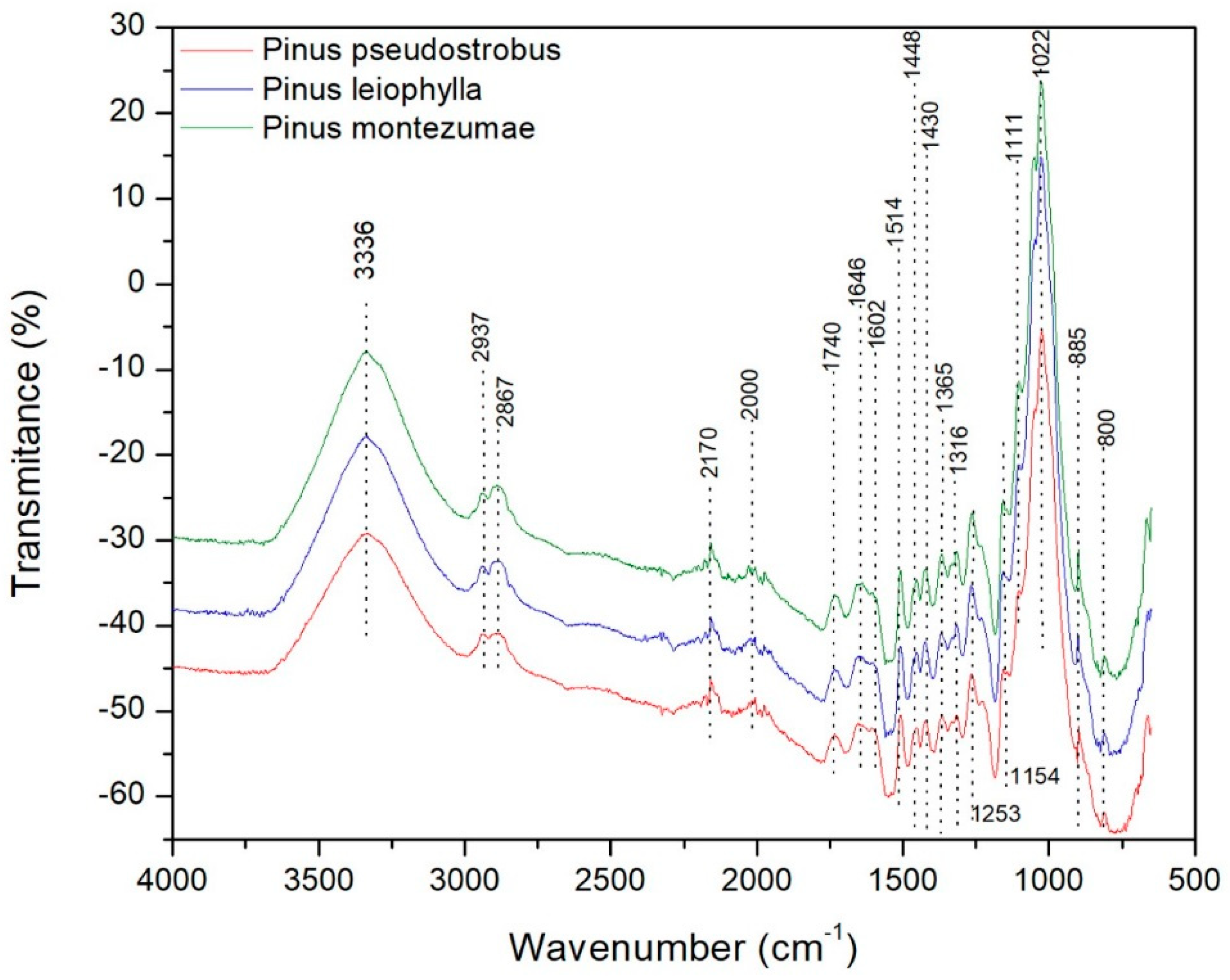
3.4. Fourier Transform Infrared Analysis (FT-IR)

The species of the wood samples, which were analyzed in this study, are P. pseudostrobus, P. leiophylla and P. montezumae. The FT-IR spectrum of the three pine species is shown in Figure 8.

The following main absorption regions may be highlighted. Firstly, bands in the range 3000 to 3500 cm⁻¹ are observed due to the O-H stress of the intermolecular hydrogen bonded. Such a region is defined for hydroxyl groups according to a certain frequency value, for example the indicated maximum of 3336 cm⁻¹. According to literature when an inter-intra-molecular combination of H₂ bonds is present, it is possible to cause an increase in the OH band of the IR [76]. In the band range between 3000 and 2700 cm⁻¹ symmetrical and non-symmetrical vibrations are associated according to the presence of methylene, methoxyl C-H and methyl groups, which are constituents of hemicellulose [77]. In the band range from 2170 to 2000 cm⁻¹ there is the presence of gases such as CO₂ and CO. When observing all the spectra, it can be observed that there is a concentration of peaks that stands out in the determined region between 800 and 1800 cm⁻¹. Such peaks represent some bands that stretch and deform to various groups and vibrational values that correspond to the constituents of the lignocellulosic material. This range represents very valuable information in lignocellulosic materials regarding changes (stretching and deformation vibrations) in the components of cellulose, hemicellulose and lignin [78]. Then, there are some absorption peaks between 1646 and 1740 cm⁻¹ corresponding to the vibrations of the carbonyl groups C=O, acetyl and carboxyl groups present in hemicellulose and cellulose [77]. The band of absorption between 1514 and 1646 cm⁻¹ is attributed to the vibrations of the groups C-O-C of the ring of the β-glucopyranosa that constitutes the cellulose. There are bands in the range of 1430–1602 cm⁻¹ corresponding to the vibration of the structure of the aromatic rings (C = C) characteristic of cellulose and lignin. When identifying the loss of acetyl-type groups, usually there is a reduction in the band with a value of 1253 cm⁻¹, as can be seen in Figure 8, which represents the vibration in C-O bonds of Ph-C, that is an important part of both the lignin aromatic ring and the xyloglucan [79]. The band present in 1154 cm⁻¹ represent the vibrational behavior of C-O-C bonds of the esters characteristic of hemicellulose and cellulose. The 1022 cm⁻¹ signal to the C-O vibration of alcohols is attributed to hemicellulose, cellulose and lignin. Finally, the bands in the range 800–895 cm⁻¹ are those corresponding to the vibration of the structure of the aromatic rings (C-C) characteristic of lignin degradation. It is important to mention that, the wavelength value equal to 1514 cm⁻¹ corresponds to the structure of the aromatic ring of the lignin, i.e., the C-C bonds [80,81]. According to those reported by other authors, glucose ring stretching vibration is found at wave number 1111 cm⁻¹ [82], which is also shown in Figure 8.

4. Conclusions

For the first time, the kinetics of the pyrolytic process of P. pseudostrobus, P. leiophylla and P. montezumae in an inert atmosphere has been studied by thermogravimetric analysis to determine its most representative kinetic parameters, such as activation energy and frequency factor. According to the TGA analysis, the most important quantitative phase of pyrolysis of the three pine species studied takes place in the 150 to 400 °C range. Approximately up to 250 °C a loss of 10 to 15% of mass occurs, corresponding to the first stage, i.e., loss of water and extractives. From 250 °C to 400 °C most of the volatile substances are released, mainly hemicellulose and cellulose being decomposed, with a loss of mass of about 80%. A rapid reduction of volatile compounds was observed at high temperatures (T > 400 °C) as well as coke formation.

The average activation energy determined by the Friedman, OFW and KAS methods was 126.58, 123.22 and 112.72 kJ/mol respectively with regard to P. pseudostrobus; 146.15, 143.24 and 132.76 kJ/mol respectively for P. leiophylla and 148.12, 151.80 and 141.25 kJ/mol, respectively, for P. montezumae, respectively, resulting in similar values in magnitude for the three methods and maintaining a tendency to increase with increasing heating velocity. For the range α = 0.20–0.70 and according to the results, it was possible to observe an optimal correlation (average R² > 0.97) in practically all the experimental data used in the mathematical models applied in this investigation to determine the Ea, in this sense, the non-consideration of some data for the calculation and analysis of Ea, it does not affect the veracity and quality of the results.

The average frequency factor (Z) for each heating rate (β) in the Friedman, KAS and OFW methods varies from 6.28 × 10⁹–3.72 × 10⁹; and 1.69 × 10⁸–1.55 × 10⁸; and 1.95 × 10⁷–2.08 × 10⁷ for P. pseudostrobus, respectively. On average, a variation of Z was found for P. leiophylla from 1.06 × 10¹⁴–4.71 × 10¹³; and 9.04 × 10⁹–8.10 × 10⁹; and 1.07 × 10⁹–1.09 × 10⁹, respectively. Finally, to P. montezumae the results of Z, were 2.65 × 10¹⁵–1.09 × 10¹⁵; and 3.88 × 10¹⁰–3.34 × 10¹⁰; and 4.61 × 10⁹–4.50 × 10⁹, respectively. When performing the kinetic analysis and taking into account the error values and the determination coefficient, it is established that the FWO and KAS models are best suited to the thermal degradation of P. pseudostrobus, P. leiophylla and P. montezumae. The variability of the Ea values when applying these methods confirm the complexity of the degradation process. Finally, it should be mentioned that the low ash content of P. pseudostrobus, P. leiophylla and P. montezumae make them good candidates for the production of biochemical products such as methane and its subsequent processing for the production of hydrogen. According to FT-IR analysis, it was observed that all relative intensities in all bands were higher for P. montezumae, followed by Pinus leiophylla and finally P. pseudostrobus. The band is mainly distinguished in the maximum peak of 1022 cm⁻¹. The differences between the IR values in the softwoods used in this research may be related to the amount of the main biochemical components of the lignocellulosic material, i.e., cellulose, hemicellulose and lignin.

References

1. Manzano, F.; Alcayde, A.; Montoya, F.; Zapata, A.; Gil, C. Scientific production of renewable energies worldwide: An overview. Renew. Sustain. Energy Rev. 2013, 18, 134–143. [Google Scholar] [CrossRef]
2. Varma, A.; Thakur, L.; Shankar, R.; Mondal, P. Pyrolysis of wood sawdust: Effects of process parameters on products yield and characterization of products. Waste Manag. 2019, 89, 224–235. [Google Scholar] [CrossRef]
3. Saldarriaga, J.; Aguado, R.; Pablos, A.; Amutio, M.; Olazar, M.; Bilbao, J. Fast characterization of biomass fuels by thermogravimetric analysis (TGA). Fuel 2015, 140, 744–751. [Google Scholar] [CrossRef]
4. Soto, N.; Machado, W.; López, D. Determinación de los parámetros cinéticos en la pirólisis del pino ciprés. Quim. Nova 2010, 33, 1500–1505. [Google Scholar] [CrossRef] [Green Version]
5. Davis, S.; Diegel, S.; Boundy, R. Transportation Energy Data Book; Oak Ridge National Laboratory: Oak Ridge, TN, USA, 2009; No. ORNL-6984.
6. Bridgwater, A. The production of biofuels and renewable chemicals by fast pyrolysis of biomass. Int. J. Glob. Energy 2007, 27, 160–203. [Google Scholar] [CrossRef]
7. Ragauskas, A.; Williams, C.; Davison, B.; Britovsek, G.; Cairney, J.; Eckert, C.; Frederick, W.; Hallett, J.; Leak, D.; Liotta, C.; et al. The path forward for biofuels and biomaterials. Science 2006, 311, 484–489. [Google Scholar] [CrossRef] [PubMed] [Green Version]
8. Frombo, F.; Minciardi, R.; Robba, M.; Rosso, F.; Sacile, R. Planning woody biomass logistics for energy production: A strategic decision model. Biomass Bioenergy 2009, 33, 372–383. [Google Scholar] [CrossRef]
9. Mullaney, H.; Farag, I.; La Claire, C.; Barrett, C. Technical, Environmental and Economic Feasibility of Bio-Oil in New Hampshire’s North Country; New Hampshire Industrial Research Center: Durham, NH, USA, 2002. [Google Scholar]
10. Da Silva, J.; Alves, J.; de Araujo, W.; Andersen, S.; de Sena, R. Pyrolysis kinetic evaluation by single-step for waste wood from reforestation. Waste Manag. 2018, 72, 265–273. [Google Scholar] [CrossRef]
11. Janković, B. The pyrolysis process of wood biomass samples under isothermal experimental conditions-energy density considerations: Application of the distributed apparent activation energy model with a mixture of distribution functions. Cellulose 2014, 21, 2285–2314. [Google Scholar] [CrossRef]
12. Mohan, D.; Pittman, C.; Steele, P. Pyrolysis of wood/biomass for bio-oil: A critical review. Energy Fuels 2006, 20, 848–889. [Google Scholar] [CrossRef]
13. Soltes, E.; Elder, T. Pyrolysis in Organic Chemicals from Biomass. IS Goldstein; CRC Press: Florida, FL, USA, 1981. [Google Scholar]
14. Branca, C.; Lannace, A.; Di Blasi, C. Devolatilization and Combustion Kinetics of Quercus cerris Bark. Energy Fuels 2007, 21, 1078–1084. [Google Scholar] [CrossRef]
15. D’ Almeida, A.; Barreto, D.; Calado, V.; d’ Almeida, J. Thermal analysis of less common lignocellulose fibers. J. Therm. Anal. Calorim. 2008, 91, 405–408. [Google Scholar] [CrossRef]
16. Guerrero, M.; da Silva, M.; Zaragoza, M.; Gutiérrez, J.; Velderrain, V.; Ortiz, A.; Collins, V. Thermogravimetric study on the pyrolysis kinetics of apple pomace as waste biomass. Int. J. Hydrogen. Energy 2014, 39, 16619–16627. [Google Scholar] [CrossRef]
17. Hill, J. For Better Thermal Analysis and Calorimetry; International Confederation for Thermal Analysis, 1991. [Google Scholar]
18. Giuntoli, J.; De Jong, W.; Arvelakis, S.; Spliethoff, H.; Verkooijen, A. Quantitative and kinetic TG-FTIR study of biomass residue pyrolysis: Dry distiller’s grains with solubles (DDGS) and chicken manure. J. Anal. Appl. Pyrol. 2009, 85, 301–312. [Google Scholar] [CrossRef]
19. Zhu, H.; Yan, J.; Jiang, X.; Lai, Y.; Cen, K. Study on pyrolysis of typical medical waste materials by using TG-FTIR analysis. J. Hazard. Mater. 2008, 153, 670–676. [Google Scholar] [CrossRef] [PubMed]
20. Koreňová, Z.; Juma, M.; Annus, J.; Markoš, J. Kinetics of pyrolysis and properties of carbon black from a scrap tire. Chem. Pap. 2006, 60, 422–426. [Google Scholar] [CrossRef]
21. Sun, J.; Wang, W.; Liu, Z.; Ma, Q.; Zhao, C.; Ma, C. Kinetic study of the pyrolysis of waste printed circuit boards subject to conventional and microwave heating. Energies 2012, 5, 3295–3306. [Google Scholar] [CrossRef] [Green Version]
22. White, J.; Catallo, W.; Legendre, B. Biomass pyrolysis kinetics: A comparative critical review with relevant agricultural residue case studies. J. Anal. Appl. Pyrol. 2011, 91, 1–33. [Google Scholar] [CrossRef]
23. Singh, S.; Wu, C.; Williams, P. Pyrolysis of waste materials using TGA-MS and TGA-FTIR as complementary characterisation techniques. J. Anal. App. Pyrol. 2012, 94, 99–107. [Google Scholar] [CrossRef]
24. Cao, R.; Naya, S.; Artiaga, R.; García, A.; Varela, A. Logistic approach to polymer degradation in dynamic TGA. Polym. Degrad. Stab. 2004, 85, 667–674. [Google Scholar] [CrossRef]
25. Brown, M. Steps in a minefield: Some kinetic aspects of thermal analysis. J. Therm. Anal. Calorim. 1997, 49, 17–32. [Google Scholar] [CrossRef]
26. Brown, M.; Maciejewski, M.; Vyazovkin, S.; Nomen, R.; Sempere, J.; Burnham, A.; Opfermann, J.; Strey, R.; Anderson, H.; Kemmler, A.; et al. Computational aspects of kinetic analysis: Part A: The ICTAC kinetics project-data, methods and results. Thermochim. Acta 2000, 355, 125–143. [Google Scholar] [CrossRef]
27. Friedman, H. Kinetics of thermal degradation of char-forming plastics from thermogravimetry. Application to a phenolic plastic. J. Polym. Sci. Pol. Sym. 1964, 6, 183–195. [Google Scholar] [CrossRef]
28. Ozawa, T. A new method of analyzing thermogravimetric data. B. Chem. Soc. Jpn. 1965, 38, 1881–1886. [Google Scholar] [CrossRef] [Green Version]
29. Kissinger, H. Reaction kinetics in differential thermal analysis. Anal. Chem. 1957, 29, 1702–1706. [Google Scholar] [CrossRef]
30. Akahira, T. Trans. Joint convention of four electrical institutes. Res. Rep. Chiba Inst. Technol. 1971, 16, 22–31. [Google Scholar]
31. Pintor, L.; Carrillo, A.; Herrera, R.; López, P.; Rutiaga, J. Physical and chemical properties of timber byproducts from Pinus leiophylla, P. montezumae and P. pseudostrobus for a bioenergetic use. Wood Res. 2017, 62, 849–862. [Google Scholar]
32. Téllez, C.; Ochoa, H.; Sanjuan, R.; Rutiaga, J. Componentes químicos del duramen de Andira inermis (W. Wright) DC. (Leguminosae). Rev. Chapingo Ser. Cienc. For. Ambient. 2010, 16, 87–93. [Google Scholar]
33. UNE-EN 14775. Solid Biofuels. Method for the Ash Content Determination; CONFEMADERA, AENOR, Grupo 9: Madrid, España, 2010; 10p. (In Spanish) [Google Scholar]
34. Vyazovkin, S.; Burnham, A.; Criado, J.; Pérez, L.; Popescu, C.; Sbirrazzuoli, N. ICTAC Kinetics Committee recommendations for performing kinetic computations on thermal analysis data. Thermochim. Acta 2011, 520, 1–19. [Google Scholar] [CrossRef]
35. Damartzis, T.; Vamvuka, D.; Sfakiotakis, S.; Zabaniotou, A. Thermal degradation studies and kinetic modeling of cardoon (Cynara cardunculus) pyrolysis using thermogravimetric analysis (TGA). Bioresour. Technol. 2011, 102, 6230–6238. [Google Scholar] [CrossRef]
36. Flynn, J. The isoconversional method for determination of energy of activation at constant heating rates: Corrections for the Doyle approximation. J. Therm. Anal. Calorim. 1983, 27, 95–102. [Google Scholar] [CrossRef]
37. Sadhukhan, A.; Gupta, P.; Saha, R. Modelling of pyrolysis of large wood particles. Bioresour. Technol. 2009, 100, 3134–3139. [Google Scholar] [CrossRef] [PubMed]
38. Min, F.; Zhang, M.; Chen, Q. Non-isothermal kinetics of pyrolysis of three kinds of fresh biomass. J. China Univ. Min. Technol. 2007, 17, 105–111. [Google Scholar] [CrossRef]
39. Capart, R.; Khezami, L.; Burnham, A. Assessment of various kinetic models for the pyrolysis of a microgranular cellulose. Thermochim. Acta 2004, 417, 79–89. [Google Scholar] [CrossRef] [Green Version]
40. Vlaev, L.; Markovska, I.; Lyubchev, L. Non-isothermal kinetics of pyrolysis of rice husk. Thermochim. Acta 2003, 406, 1–7. [Google Scholar] [CrossRef]
41. Galwey, A.; Brown, M. Application of the Arrhenius equation to solid state kinetics: Can this be justified? Thermochim. Acta 2002, 386, 91–98. [Google Scholar] [CrossRef]
42. Steinfeld, J.; Francisco, J.; Hase, W. Chemical Kinetics and Dynamics, 2nd ed.; Prentice-Hall: Upper Saddle River, NJ, USA, 1999. [Google Scholar]
43. Atkins, P.W. Physical Chemistry, 5th ed.; W.H. Freeman: New York, NY, USA, 1994. [Google Scholar]
44. Flynn, J. The ‘temperature integral’—Its use and abuse. Thermochim. Acta 1997, 300, 83–92. [Google Scholar] [CrossRef]
45. Liu, M.; Gao, L.; Zhao, Q.; Wang, Y.; Yang, X.; Cao, S. Thermal degradation process and kinetics of poly (dodecamethyleneisophthalamide). Chem. J. Internet. 2003, 5, 43. [Google Scholar]
46. Biagini, E.; Guerrini, L.; Nicolella, C. Development of a variable activation energy model for biomass devolatilization. Energy Fuels 2009, 23, 3300–3306. [Google Scholar] [CrossRef]
47. Kantarelis, E.; Yang, W.; Blasiak, W.; Forsgren, C.; Zabaniotou, A. Thermochemical treatment of E-waste from small household appliances using highly pre-heated nitrogen-thermogravimetric investigation and pyrolysis kinetics. Appl. Energy 2011, 88, 922–929. [Google Scholar] [CrossRef]
48. Flynn, J.; Wall, L. General treatment of the thermogravimetry of polymers. J. Res. Nat. Bur. Stand. 1966, 70, 487–523. [Google Scholar] [CrossRef] [PubMed]
49. Tang, T.; Chaudhri, M. Analysis of dynamic kinetic data from solid-state reactions. J. Therm. Anal. Calorim. 1980, 18, 247–261. [Google Scholar] [CrossRef]
50. Doyle, C. Kinetic analysis of thermogravimetric data. J. Appl. Polym. Sci. 1961, 5, 285–292. [Google Scholar] [CrossRef]
51. Chao, M.; Li, W.; Wang, X. Influence of antioxidant on the thermal–oxidative degradation behavior and oxidation stability of synthetic ester. Thermochim. Acta 2014, 591, 16–21. [Google Scholar] [CrossRef]
52. Coats, A.; Redfern, J. Kinetic parameters from thermogravimetric data. Nature 1964, 201, 68–69. [Google Scholar] [CrossRef]
53. Lyon, R. An integral method of nonisothermal kinetic analysis. Thermochim. Acta 1997, 297, 117–124. [Google Scholar] [CrossRef]
54. Obernberger, I.; Thek, G. The Pellet Handbook, 1st ed.; Earthscan: London, UK; Washington, DC, USA, 2010. [Google Scholar]
55. Van Lith, S.; Alonso, V.; Jensen, P.; Frandsen, F.; Glarborg, P. Release to the gas phase of inorganic elements during wood combustion. Part 1: Development and evaluation of quantification methods. Energy Fuels 2006, 20, 964–978. [Google Scholar] [CrossRef]
56. Werkelin, J.; Lindberg, D.; Boström, D.; Skrifvars, B.; Hupa, M. Ash-forming elements in four Scandinavian wood species part 3: Combustion of five spruce samples. Biomass Bioenergy 2011, 35, 725–733. [Google Scholar] [CrossRef]
57. Miles, T. Alkali Deposits Found in Biomass Power Plants; NREL Report 443-8142; Vol 1. Sand 96-8225; National Techrucd Momation Service (NTIS): Springfield, VA, USA, 1995. [Google Scholar]
58. Du, Z.; Sarofim, A.; Longwell, J. Activation energy distribution in temperature-programmed desorption: Modeling and application to the soot oxygen system. Energy Fuels 1990, 4, 296–302. [Google Scholar] [CrossRef]
59. Yahiaoui, M.; Hadoun, H.; Toumert, I.; Hassani, A. Determination of kinetic parameters of Phlomis bovei de Noé using thermogravimetric analysis. Bioresour. Technol. 2015, 196, 441–447. [Google Scholar] [CrossRef]
60. Vamvuka, D.; Kakaras, E.; Kastanaki, E.; Grammelis, P. Pyrolysis characteristics and kinetics of biomass residuals mixtures with lignite. Fuel 2003, 82, 1949–1960. [Google Scholar] [CrossRef]
61. Meesri, C.; Moghtaderi, B. Lack of synergetic effects in the pyrolytic characteristics of woody biomass/coal blends under low and high heating rate regimes. Biomass Bioenergy 2002, 23, 55–66. [Google Scholar] [CrossRef]
62. Jeguirim, M.; Trouvé, G. Pyrolysis characteristics and kinetics of Arundo donax using thermogravimetric analysis. Bioresour. Technol. 2009, 100, 4026–4031. [Google Scholar] [CrossRef] [PubMed]
63. Gašparovič, L.; Koreňová, Z.; Jelemenský, Ľ. Kinetic study of wood chips decomposition by TGA. Chem. Pap. 2010, 64, 174–181. [Google Scholar] [CrossRef]
64. Quan, C.; Li, A.; Gao, N. Thermogravimetric analysis and kinetic study on large particles of printed circuit board wastes. Waste Manag. 2009, 29, 2353–2360. [Google Scholar] [CrossRef]
65. Kumar, A.; Wang, L.; Dzenis, Y.; Jones, D.; Hanna, M. Thermogravimetric characterization of corn stover as gasification and pyrolysis feedstock. Biomass Bioenergy 2008, 32, 460–467. [Google Scholar] [CrossRef]
66. Wang, G.; Li, W.; Li, B.; Chen, H. TG study on pyrolysis of biomass and its three components under syngas. Fuel 2008, 87, 552–558. [Google Scholar] [CrossRef]
67. Mishra, R.; Mohanty, K. Pyrolysis kinetics and thermal behavior of waste sawdust biomass using thermogravimetric analysis. Bioresour. Technol. 2018, 251, 63–74. [Google Scholar] [CrossRef]
68. Vyazovkin, S.; Wight, C. Model-free and model-fitting approaches to kinetic analysis of isothermal and nonisothermal data. Thermochim. Acta 1999, 340, 53–68. [Google Scholar] [CrossRef]
69. Amutio, M.; Lopez, G.; Aguado, R.; Artetxe, M.; Bilbao, J.; Olazar, M. Kinetic study of lignocellulosic biomass oxidative pyrolysis. Fuel 2012, 95, 305–311. [Google Scholar] [CrossRef]
70. Domínguez, J.; Santos, T.; Rigual, V.; Oliet, M.; Alonso, M.; Rodriguez, F. Thermal stability, degradation kinetics, and molecular weight of organosolv lignins from Pinus radiata. Ind. Crop. Prod. 2018, 111, 889–898. [Google Scholar] [CrossRef]
71. Vyazovkin, S. Computational aspects of kinetic analysis.: Part C. The ICTAC Kinetics Project-the light at the end of the tunnel? Thermochim. Acta 2000, 355, 155–163. [Google Scholar] [CrossRef]
72. Aboyade, A.; Hugo, J.; Carrier, M.; Meyer, E.; Stahl, R.; Knoetze, J.; Görgens, J. Non-isothermal kinetic analysis of the devolatilization of corn cobs and sugar cane bagasse in an inert atmosphere. Thermochim. Acta 2011, 517, 81–89. [Google Scholar] [CrossRef]
73. Gai, C.; Dong, Y.; Zhang, T. The kinetic analysis of the pyrolysis of agricultural residue under non-isothermal conditions. Bioresour. Technol. 2013, 127, 298–305. [Google Scholar] [CrossRef] [PubMed]
74. Huang, Y.; Kuan, W.; Chiueh, P.; Lo, S. A sequential method to analyze the kinetics of biomass pyrolysis. Bioresour. Technol. 2011, 102, 9241–9246. [Google Scholar] [CrossRef]
75. Turmanova, S.; Genieva, S.; Dimitrova, A.; Vlaev, L. Non-isothermal degradation kinetics of filled with rise husk ash polypropene composites. Express Polym. Lett. 2008, 2, 133–146. [Google Scholar] [CrossRef]
76. Kondo, T. Hydrogen Bonds in Cellulose and Cellulose. Derivatives, Polysaccharides II—Structural Diversity and Functional Versatility; Dumitriu, S., Ed.; Marcel Dekker: New York, NY, USA, 2005; Chapter 3. [Google Scholar]
77. Popescu, C.; Popescu, M.; Vasile, C. Structural analysis of photodegraded lime wood by means of FT-IR and 2D IR correlation spectroscopy. Int. J. Biol. Macromol. 2011, 48, 667–675. [Google Scholar] [CrossRef]
78. Baeza, J.; Freer, J. Chemical characterization of wood and its components. In Wood and Cellulosic Chemistry; Hon, D.-S., Shiraishi, N., Eds.; Marcel Dekker Inc.: New York, NY, USA, 2001; Chapter 8; pp. 275–384. [Google Scholar]
79. Popescu, C.; Popescu, M.; Vasile, C. Characterization of fungal degraded lime wood by FT-IR and 2D IR correlation spectroscopy. Microchem. J. 2010, 95, 377–387. [Google Scholar] [CrossRef]
80. Xu, C.; Etcheverry, T. Hydro-liquefaction of woody biomass in sub-and super-critical ethanol with iron-based catalysts. Fuel 2008, 87, 335–345. [Google Scholar] [CrossRef]
81. Kim, J.; Hwang, H.; Oh, S.; Kim, Y.; Kim, U.; Choi, J. Investigation of structural modification and thermal characteristics of lignin after heat treatment. Int. J. Biol. Macromol. 2014, 66, 57–65. [Google Scholar] [CrossRef]
82. Popescu, M.; Froidevaux, J.; Navi, P.; Popescu, C. Structural modifications of Tilia cordata wood during heat treatment investigated by FT-IR and 2D IR correlation spectroscopy. J. Mol. Struct. 2013, 1033, 176–186. [Google Scholar] [CrossRef]
Figure 1. TGA curves and percent mass loss of P. pseudostrobus (A), P. leiophylla (B) and P. montezumae (C) under N2 at different heating rates.
Energies 13 00969 g001
Figure 2. DTG of P. pseudostrobus (A), P. leiophylla (B) and P. montezumae (C) under N2 at different heating rates.
Energies 13 00969 g002
Figure 3. Isothermal residence time effect for the P. pseudostrobus (A), P. leiophylla (B) and P. montezumae (C) under N2 at different heating rates.
Energies 13 00969 g003
Figure 4. Determination of activation energy by the Friedman method of Pinus pseudostrobus (A), Pinus leiophylla (B) and Pinus montezumae (C).
Energies 13 00969 g004
Figure 5. Determination of activation energy by the FWO method of Pinus pseudostrobus (A), Pinus leiophylla (B) and Pinus montezumae (C).
Energies 13 00969 g005
Figure 6. Determination of activation energy by the KAS method of Pinus pseudostrobus (A), Pinus leiophylla (B) and Pinus montezumae (C).
Energies 13 00969 g006
Figure 7. Behavior of Ea as a function of α for the three kinetic models applied of Pinus pseudostrobus (A), Pinus leiophylla (B) and Pinus montezumae (C).
Energies 13 00969 g007
Figure 8. FT-IR of Pinus pseudostrobus, Pinus leiophylla and Pinus montezumae.
Energies 13 00969 g008