1. Introduction
The growing global population leads to an increasing need for resources—food, energy, and materials. This expanding demand forces the shift from a fossil-based linear economy to a sustainable biobased economy. Bioeconomy demands biological feedstock that has the potential to generate a spectrum of bio-based products by involving multidisciplinary areas of science, management, and engineering [
1]. Agriculture is the primary supply of nutrition and bioenergy and a substantial contributor to the bioeconomy. Yet, agriculture is also linked with environmental, economic, and social aspects of climate change. For example, climate change affects the productivity of the agriculture sector, and thus change in the agricultural practices feedback to the greenhouse gas (GHG) balance. Therefore, climate change and agriculture are linked by complex relations, which can be difficult to define or measure [
2].
The vast majority of the studies that are looking into the quantification of the climate impacts use the Global Warming Potential (GWP) for a 100-year time horizon as the default metrics. Since the development of GWP metric in the early nineties, there have been updates only on the numerical value of this metric, rather than the development of the assessment methodology itself [
3].
The use of GWP is an accepted measure within the Kyoto Protocol to the United Nations Framework Convention on Climate Change as a measure to weigh the impact of climate due to the emissions of GHGs. Although the use of GWP has received various criticism due to underlying assumptions, it became widely accepted measure because of transparency and ease of use [
4]. There were numerous alternative methods developed to substitute use of GWP, such as Global Temperature Change Potential (GTP) by Shine et al. [
4], Global Warming Potential using cumulative CO2 forcing-equivalent (GWP*) by Allen et al. [
5] and other normalized point and integration metrics (see the review by Levasseur et al. [
6]). Current studies on climate science show that processes occurring in the natural environment sometimes cannot be reasonably well quantified using a single value for measuring the impact created in the 100-year perspective. This quantification using a single value cannot be done due to the non-linear nature of the emission dissipation in various environments that leads to spatial and temporal heterogeneities. Misinterpretation of these effects can lead to policy decisions that underestimate the impacts of the emissions with a short lifetime and with a dominating local pollution effect. An example of this phenomenon is given in the thesis work by Shimako [
7] and published in the paper by Shimako et al. [
8]. This work shows that the same amount of emissions might have different influence if the timing of emissions is considered. Another limitation of GWP is that it estimates the forcing of the climate but does not characterize the impact of climate dynamics. Although climate dynamics are included in the global temperature change potentials (GTPs), they are not intended to illustrate the influence of radiative forcing and enable a qualitative interpretation of causes [
9].
The GWP, including the Bern Carbon Cycle Model (BCCM), was proposed as an alternative method to take into consideration both amount and time of emission, as well as the fraction of emissions remaining in the atmosphere from previous emission periods. Furthermore, BCCM considers the effect of GHG emissions estimated as a continuous pattern that handles removals (via sinks) and addition of new emissions to the “stock” of the atmosphere hence also considering the climate system response to emissions.
Thus, this study aims to compare two methods for GHG emission accounting from the agriculture sector. Firstly, the constant GWP values for a 100-year time horizon (GWP100) and, secondly, the time dynamic GWP values for a 100-year time horizon obtained by using the BCCM to find whether the obtained results will lead to similar or contradicting conclusions. Also, the effect of global temperature potential (GTP) of the studied system is summarized.
The agriculture sector is the world’s leading source of non-CO
2 GHG emissions and the second-largest GHGs emission source overall. On the global scale, in 2010, the non-CO
2 GHG emissions from agriculture accounted for 10–12% of the total annual anthropogenic emissions or 5.2–5.8 Gt CO
2 eq. [
10]. The same share of the GHGs emissions from agriculture is also evident in the European Union (EU), where 0.442 Gt CO
2 eq. originated from agriculture that corresponds to around 10% of the total annual GHG emissions in the EU. Based on the EU strategy for a low-carbon economy by 2050 [
11], non-CO
2 GHG emissions or GHG emissions not covered by the EU Emissions Trading Scheme (non-ETS) should be cut down by 30% in the comparison to the emission in 2005 [
12]. Thus, these emission reductions should also substantially relay on the emission cutbacks in the agriculture sector. Therefore, a lot of research is put into the evaluation of emission mitigation potential in the EU Member states, including a detailed analysis of the agriculture sector [
13,
14].
3. Results and Discussion
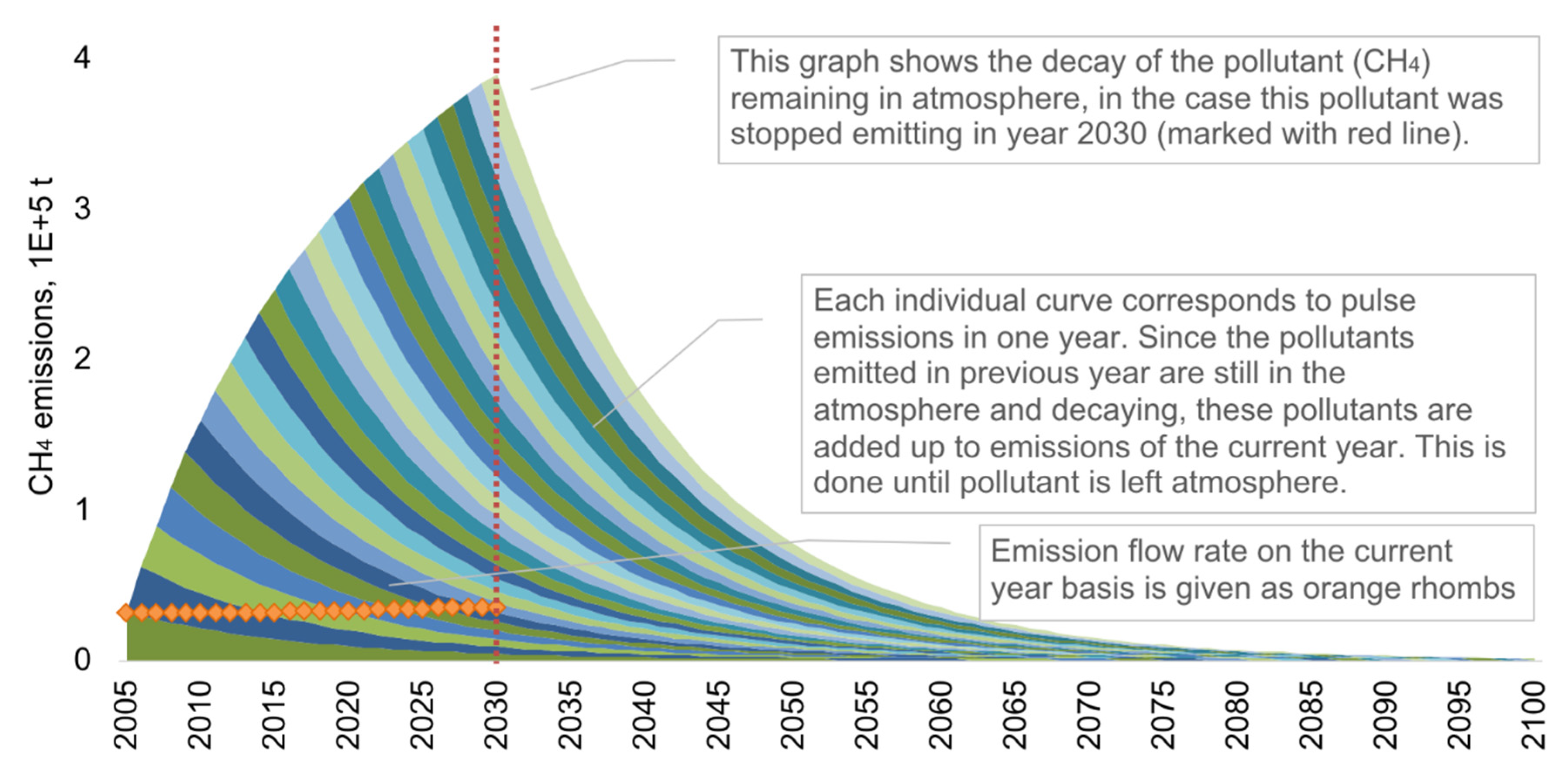
The temporal effects of the annual emissions on the current year basis and the cumulative effect of this flow in the atmosphere for both continued emission flow and the eliminated emission flow are given in
Figure 9.
In
Figure 9, each curve represents the annual pulse emissions. Since the pollutants emitted in previous years are still in the atmosphere and decaying (see
Figure 4 for individual emission decay trendlines), these pollutants are added up to emissions of the current year. The accumulation of these pulse emissions is continued until the pollutant has converged to zero concentration.
As can be seen in
Figure 9, the flow rate of emission on the current year basis is relatively lower than the amount of the total cumulative emission in the air from the previous years. From this observation, two essential conclusions can be given. First, the importance to account and reduce also “small” amounts of emissions since these “small” amounts add up to a more significant cumulative effect. And second, the interference in the flow of the emissions will have a “visible” affect only a couple of decades later, since it takes time to decay emissions already accumulated in the atmosphere.
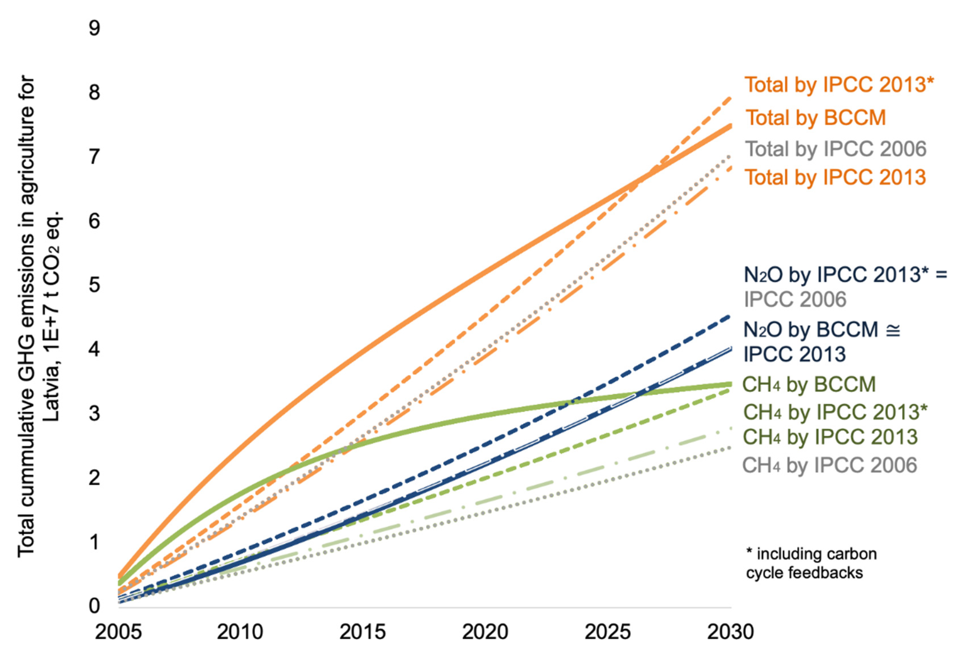
The cumulative GHG emissions calculated using the GWP100 values from the IPCC fourth [
16] and fifth [
15] assessment report and the emissions calculated using the decay function from BCCM show more substantial disparities in a shorter time horizon. At the same time, these disparities reduce in a longer time horizon (see
Figure 10).
The use of the latest GWP100 values from IPCC 2013, which include carbon cycle feedback [
15], results in emission curves located closer to the curves obtained with BCCM than the use of GWP100 values taken from IPCC 2006 [
16]. Especially significant convergence towards numbers obtained by BCCM is evident for CH
4 emissions using IPCC 2013 values instead of IPCC 2006 values. As one of the thought-provoking differences between results in IPCC and BCCM methods, the different nature of the line shapes should be stressed out. Since CH
4 decay has an evident non-linear nature, the most significant difference in the results is created in the near-term estimates of the CH
4 impacts. Similar findings are given in the work by Allen et al. [
5], where the most significant misrepresentation of the impacts using GWP is evident in the case of methane and aerosol emissions. In
Figure 10, this difference is given between the straight lines of IPCC 2006 and IPCC 2018 results and the non-linear line of BCCM results. Where an almost twofold difference is created in the short-term analysis, this difference cannot also be compensated with overestimated N
2O impacts, because N
2O results by BCCM follow a linear nature until 2030 relatively tightly.
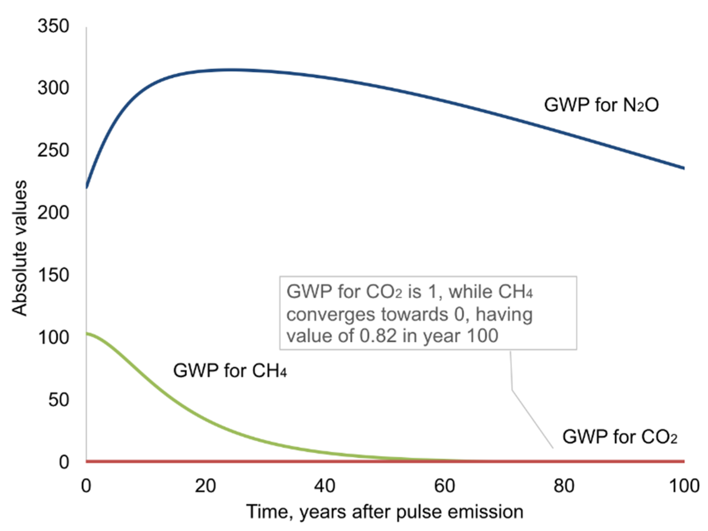
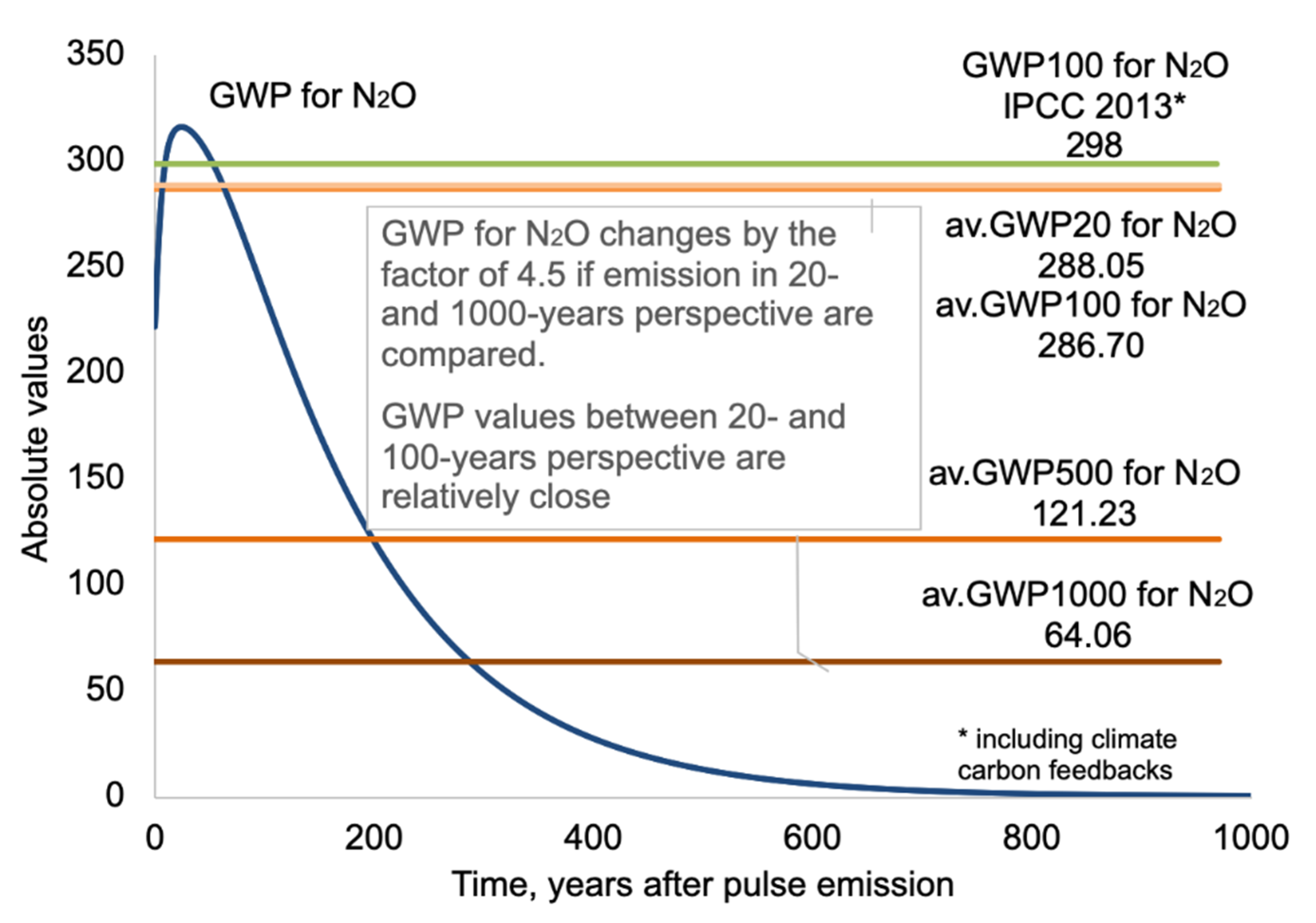
These differences in the total cumulative amounts of GHG emissions are due to the use of constant GWP values in the IPCC methodology, while in decay function, the GWP value changes with time; see
Figure 11 for GWP values for N
2O emissions and
Figure 12 for CH
4 emissions.
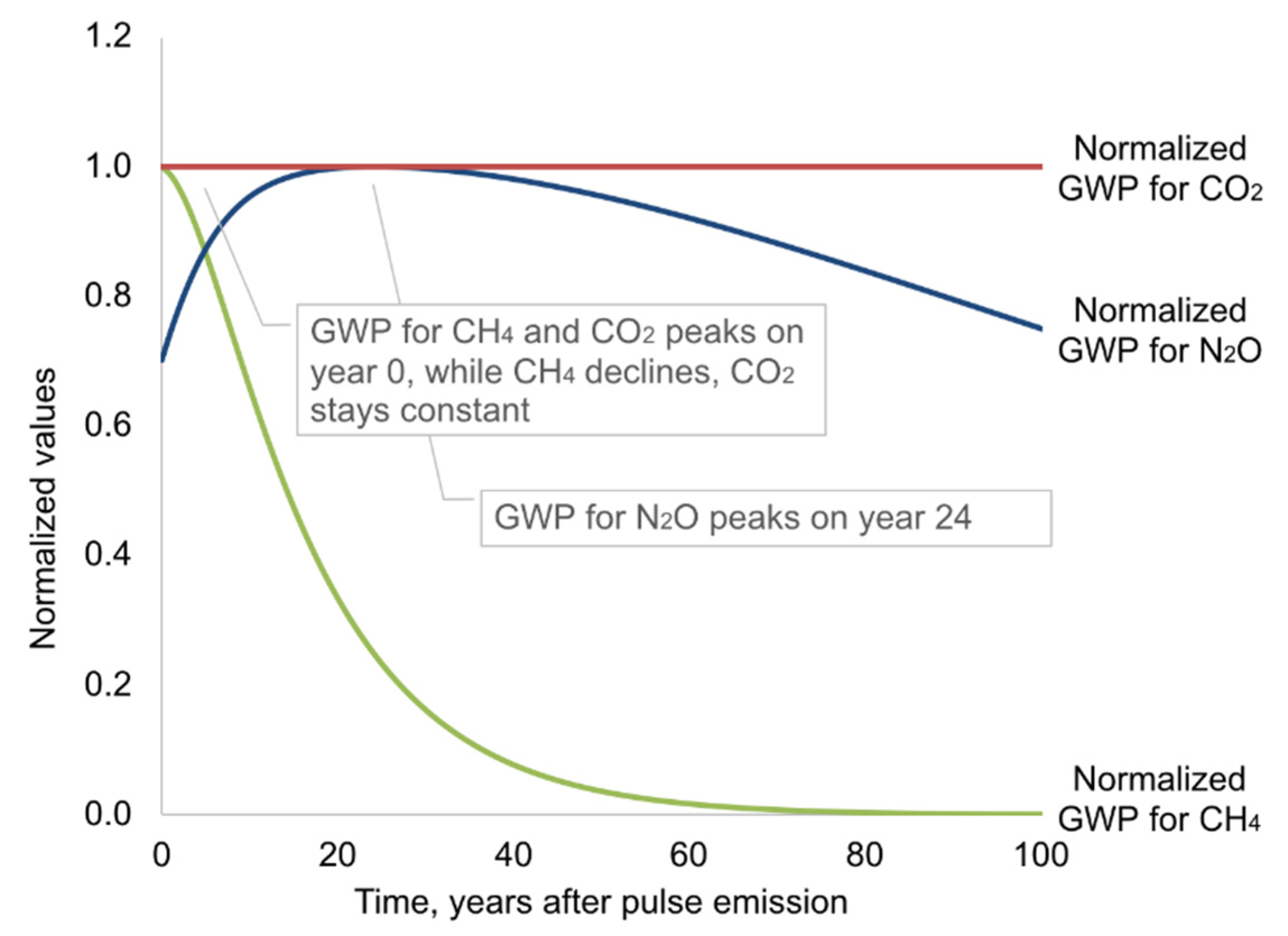
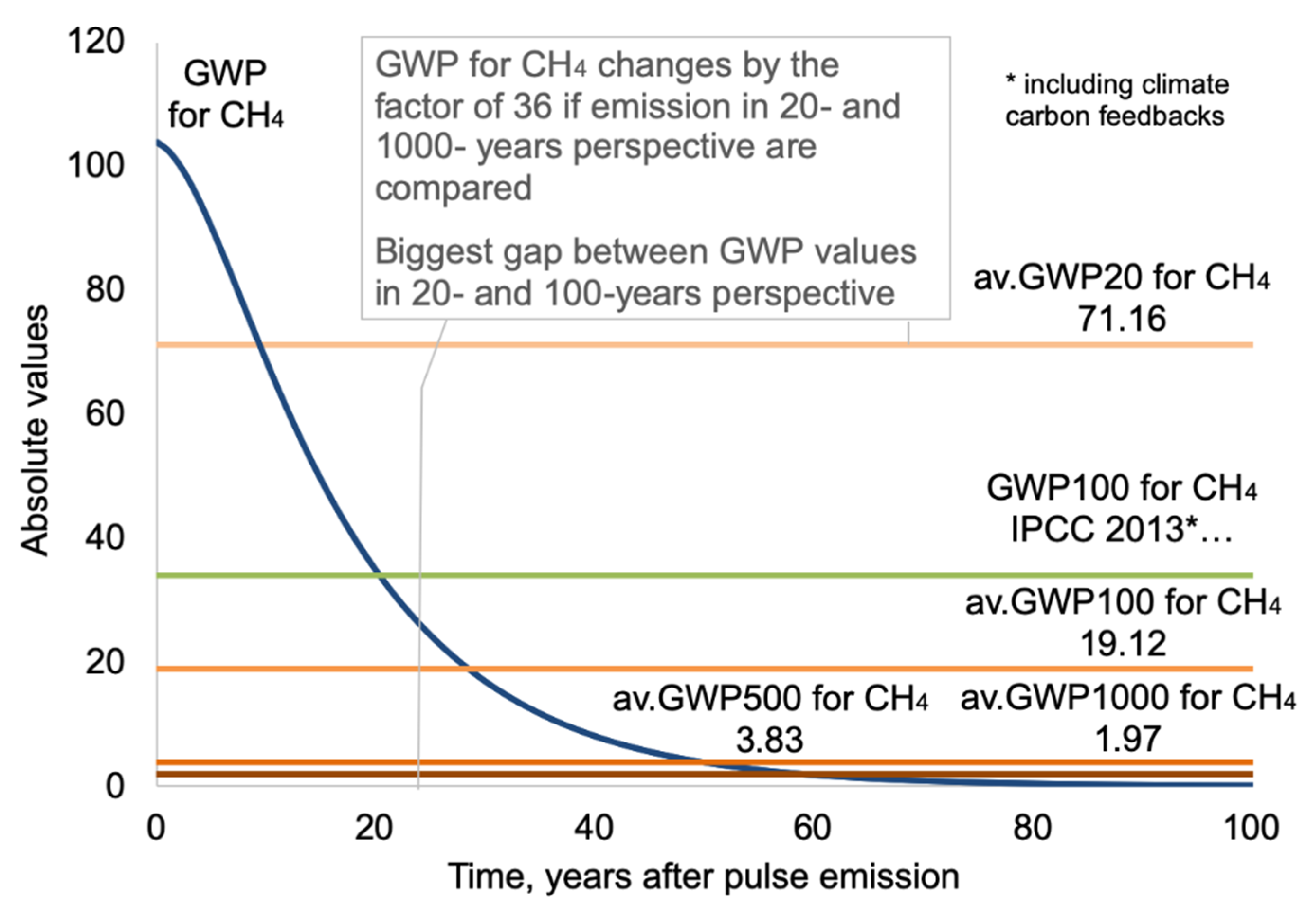
The high sensitivity of the GWP values for the chosen time frame for CH
4 and N
2O is due to the non-linear nature and different mathematical functions used for approximation of these decay functions. The difference in the average values of GWP for different time horizons can be substantial, and the obtained conclusions can be misleading. When using these averages, a situation is also possible when a longer time horizon diminishes the importance of local and relatively short lifetime emissions, such as CH
4. For example, the described situation is evident that in the case of N
2O emissions, the time frame of 20 or 100 years does not change the applied GWP values so significantly as they change in the case when CH
4 is assessed either in 20 or 100 years (see
Figure 12).
Also, the perturbation time of CH
4 emissions is approximately ten times less than the perturbation time of N
2O emissions. Thus, the use of single metrics for such different behaviour is rather challenging. The difference in the emissions’ trendlines, given in
Figure 10, between the GWP values from IPCC and the values from BCCM is visually explained in
Figure 11 and
Figure 12, where GWP100 values used in IPCC2013 for N
2O and CH
4 emissions graphically are located between different segments. In
Figure 11, for N
2O emissions, the value of GWP100 from IPCC2013 is 298, including carbon cycle feedbacks. This value of 298 is higher than the mathematical average of GWP20 and GWP100 values for N
2O. While for CH
4 emissions given in
Figure 12, the value of GWP100 from IPCC2013 is 34, including carbon cycle feedbacks. This value of 34 is in between the mathematical average of GWP20 and GWP100 values for CH
4. Thus, these selected GWP100 values from IPCC describe different segments of the emission decay period for N
2O and CH
4 and, therefore, create differences in the obtained results.
Also, longer time horizons, in general, give lower GWP values. Thus, it is always better to select a longer time horizon to have a smaller impact, but does it provide a reasonable picture of these impacts? It can be further discussed, how can the assessment of the impact at the government or enterprise-level reasonably give an interpretation for the values of the possible impacts in 100 or 500 years? And how realistic is it that the cost of these created impacts in 100 or even in the next 20 years will be adequately attributed to the producer or consumer of today? In
Figure 10, the total cumulative GHG emissions calculated using GWP values suggested by the IPCC and decay functions are compared until 2030. Usually, the comparison is used to show the created impact. In fact, the effect of the emissions occurring in the last year (2030) and a couple of years before 2030 are not included in the calculations when using the decay function. For the more realistic impacts, see
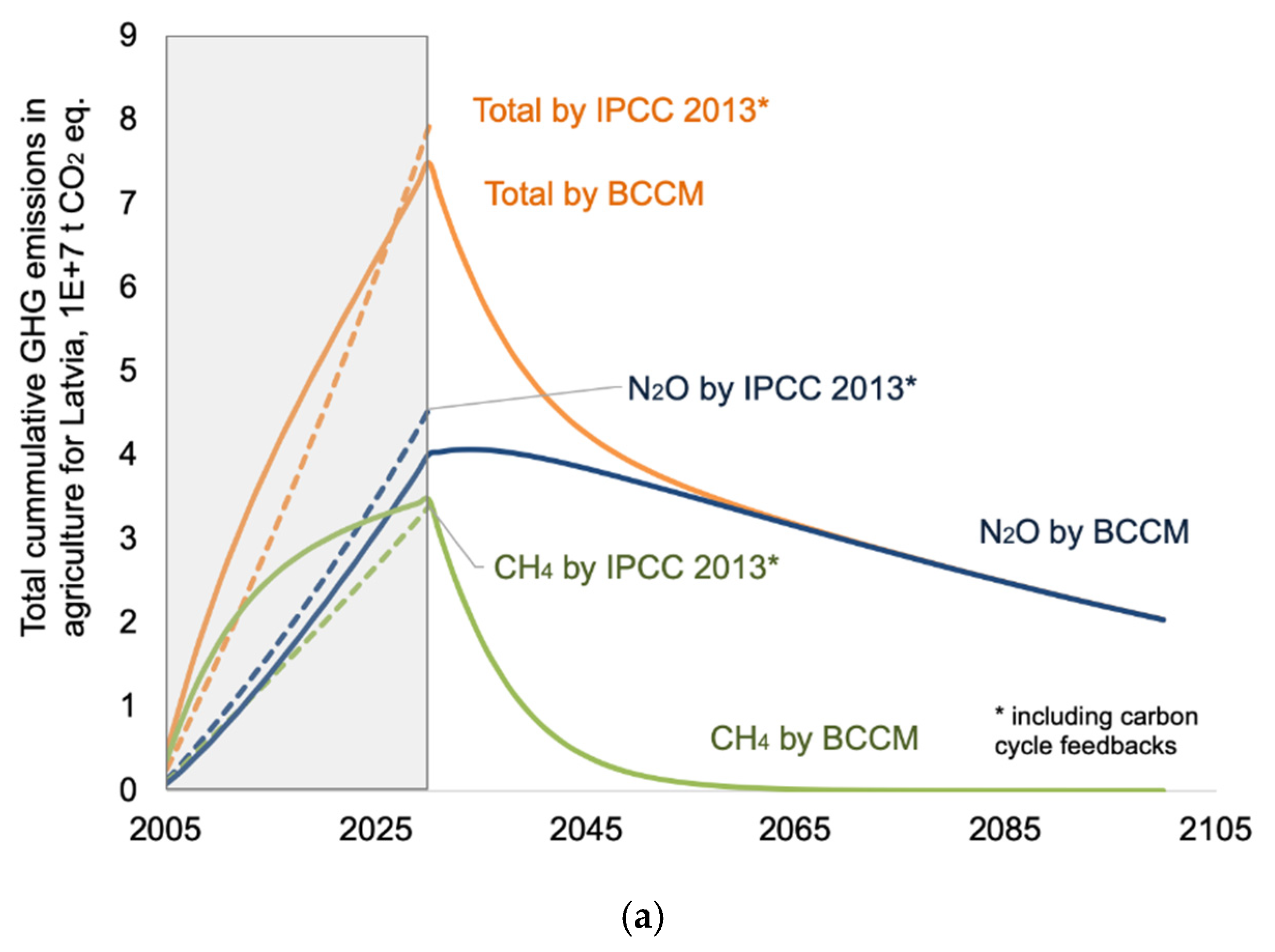
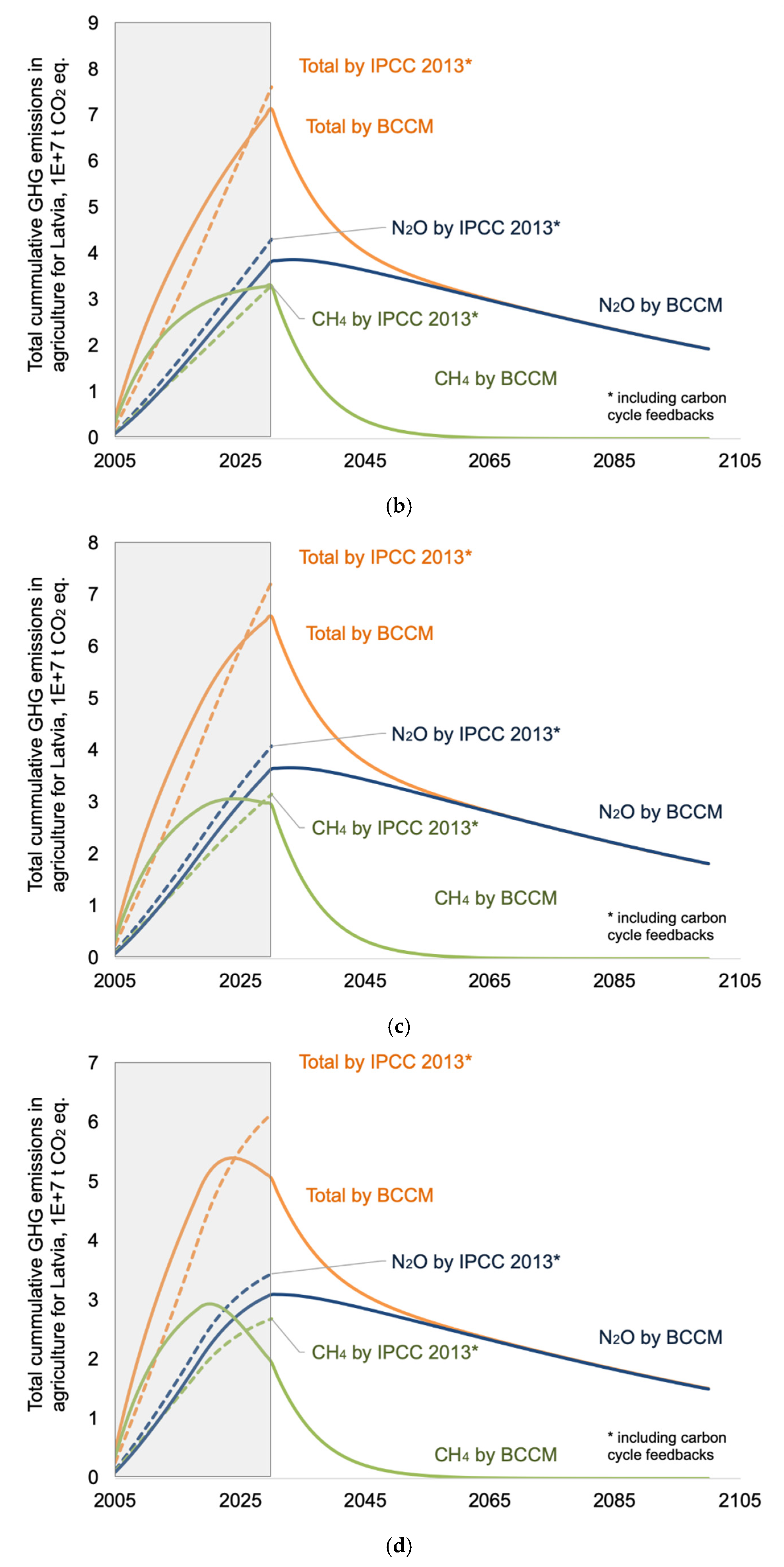
Figure 13a.
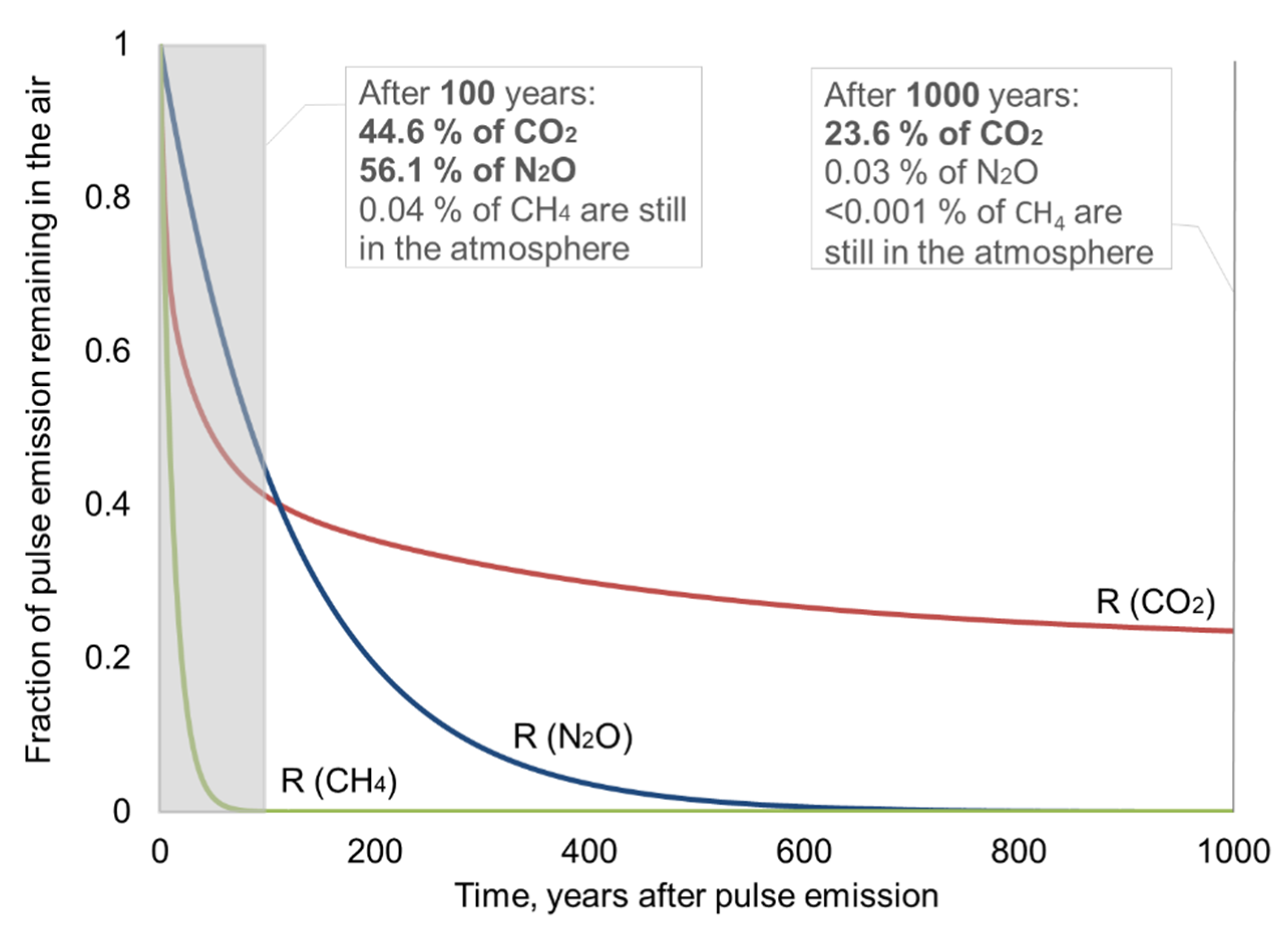
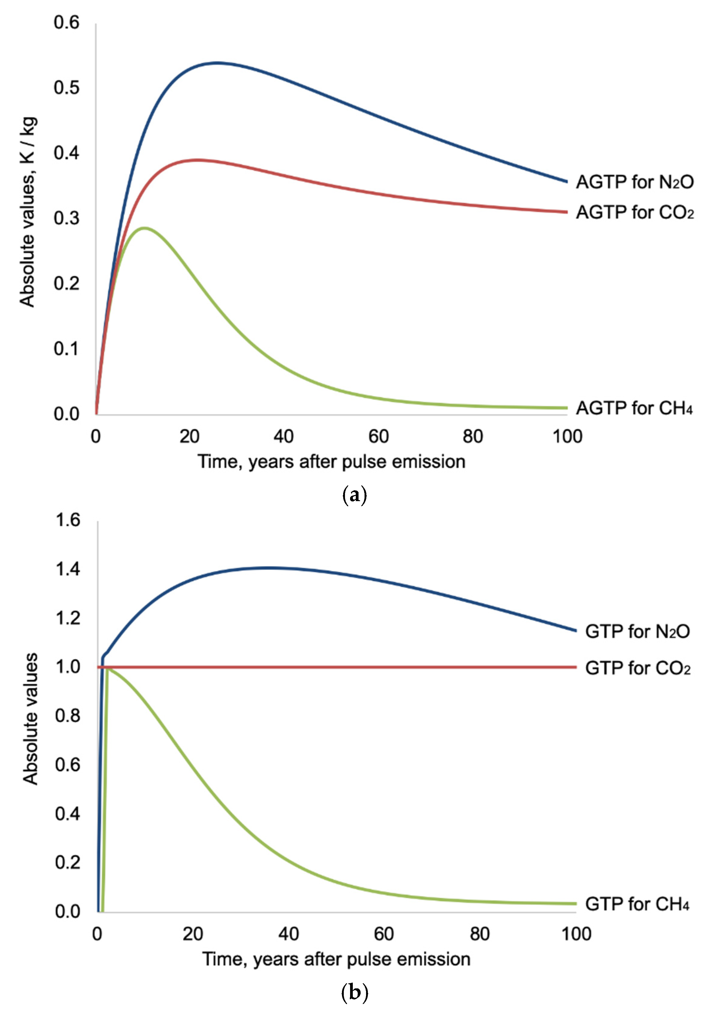
Assuming that after the year 2030, no more emissions are occurring,
Figure 13a shows how the amounts of the emissions released to the atmosphere until 2030 slowly decay. The figure shows that the fraction remaining in the air of various GHG emissions varies by nature. For CH
4, the decay is much faster, while N
2O has not even halved since its release. Similar findings of the lack of appropriate comparison between short-lived GHGs (in this case, CH
4) and long-lived GHGs (N
2O) are discussed in work by Boucher et al. [
30]. The authors explain that difficulty in using GWP for short-lived GHGs is because the GWP value does not consider that the radiative forcing of these short-lived GHGs has time to relax and reach equilibrium in the analyzed time horizon. Thus, Boucher et al. [
30] have introduced the GTP concept that generalizes climate impacts and considers different climate responses for both short and long-lived GHG emissions.
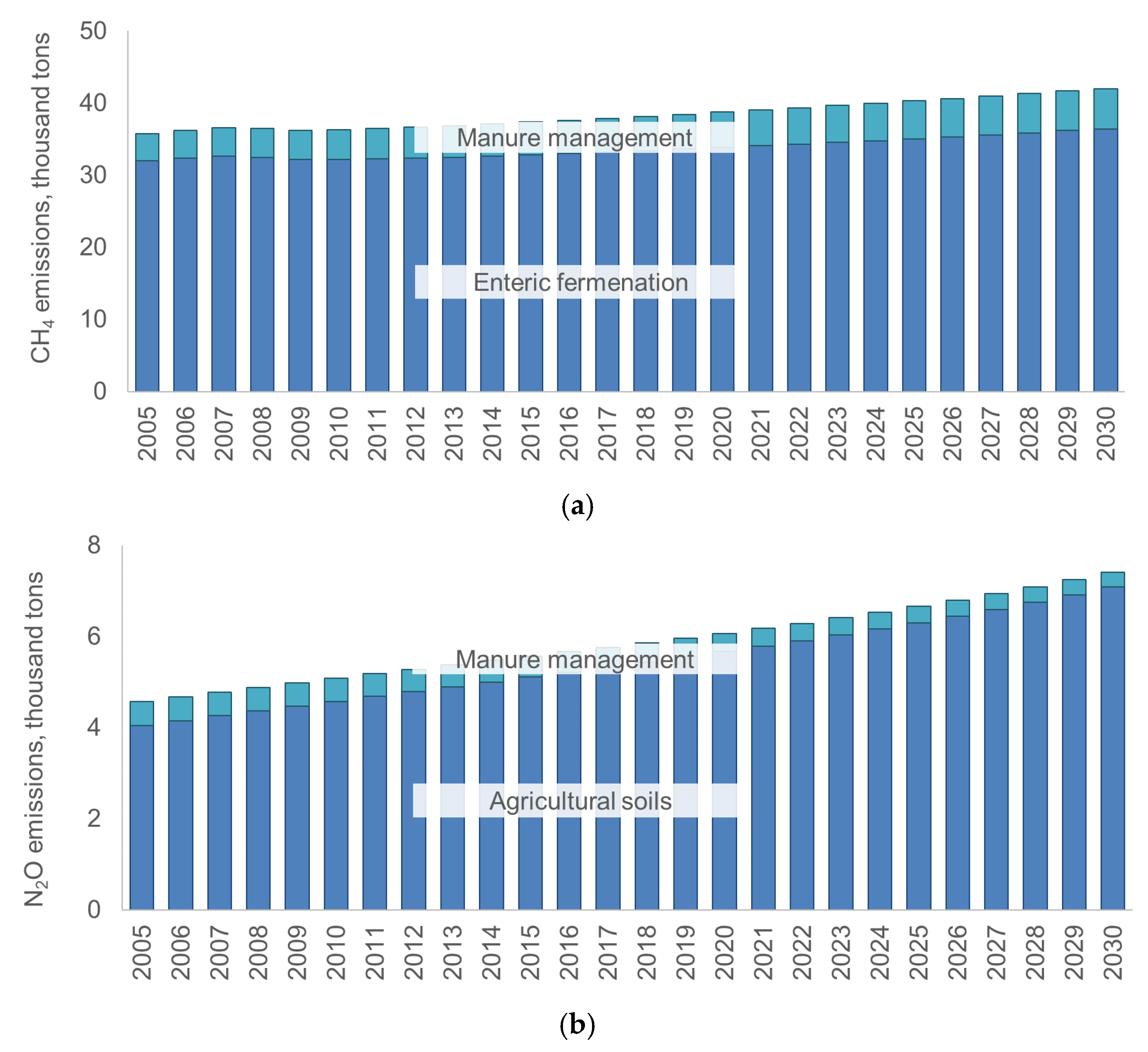
The faster decay of CH
4 is usually used as the argument to reduce the importance of this emission, especially in the agriculture sector, where CH
4 emissions have a significant share in the total impact categories; see
Figure 14a,b.
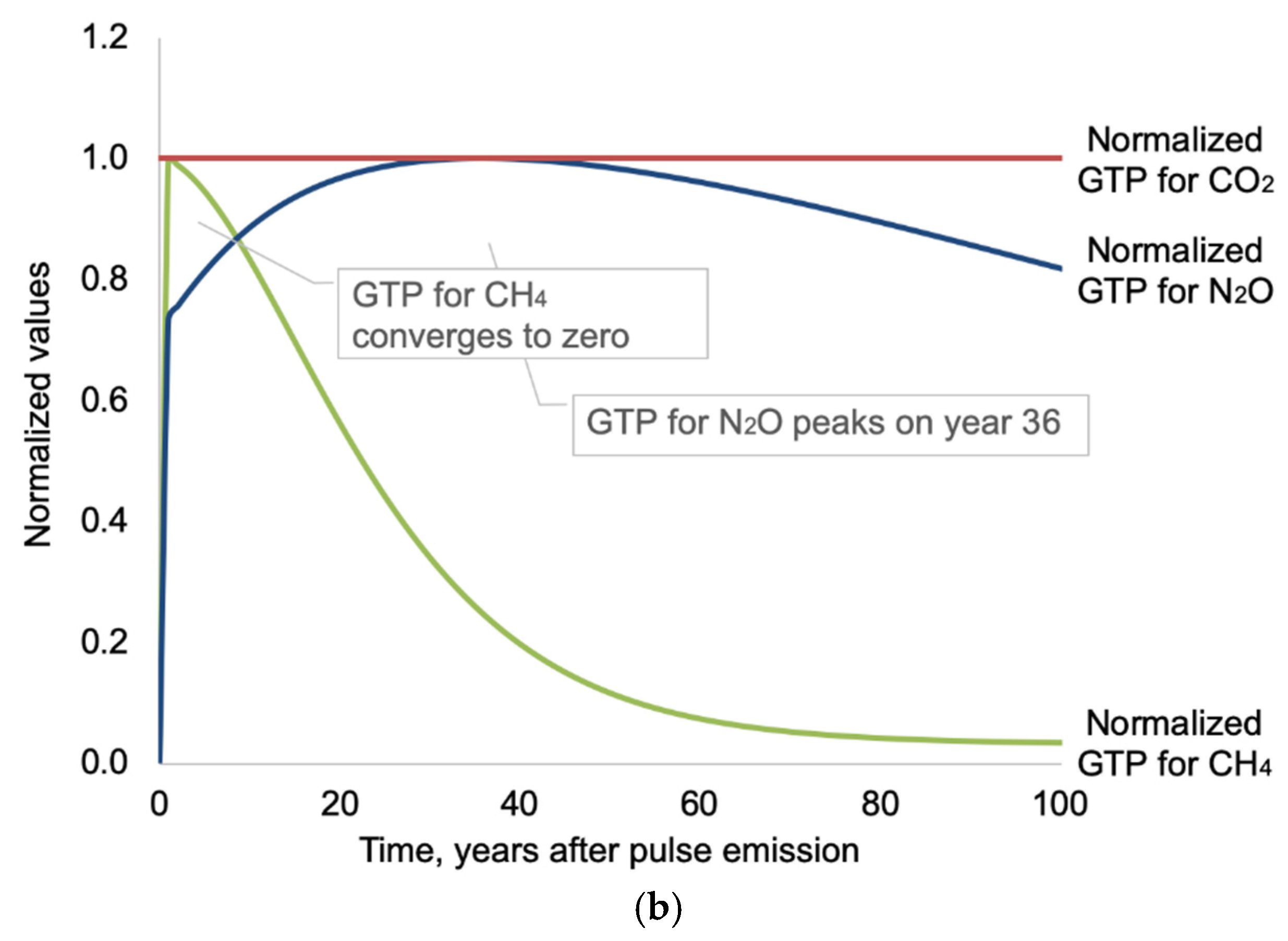
If the impact on the GTP from CH
4 is assessed, it can be seen that CH
4 shows a more obvious temperature change effect in a shorter run and, in total, contributes to more than half of the temperature change effect created by the agriculture in Latvia, as given in
Figure 14.
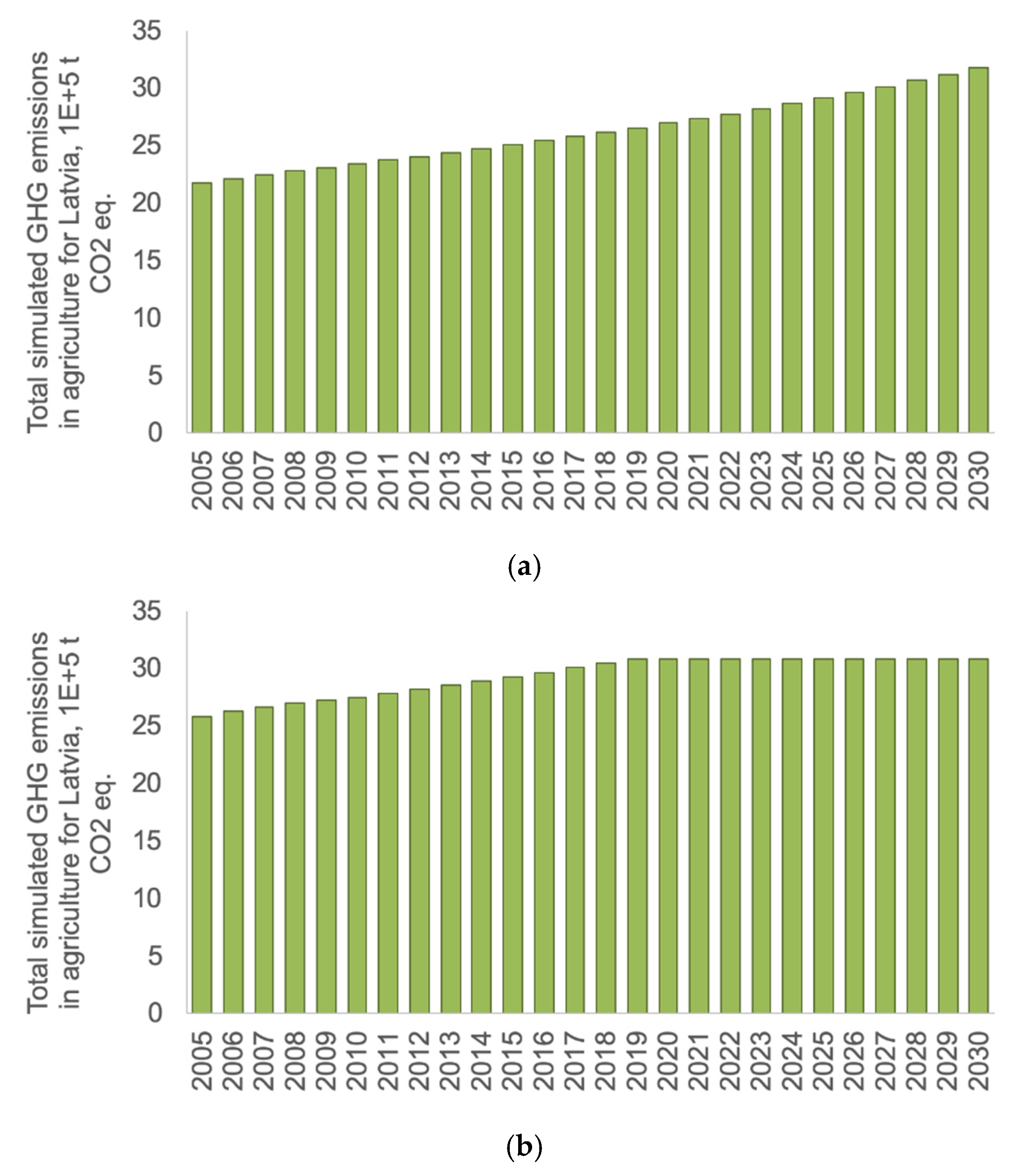
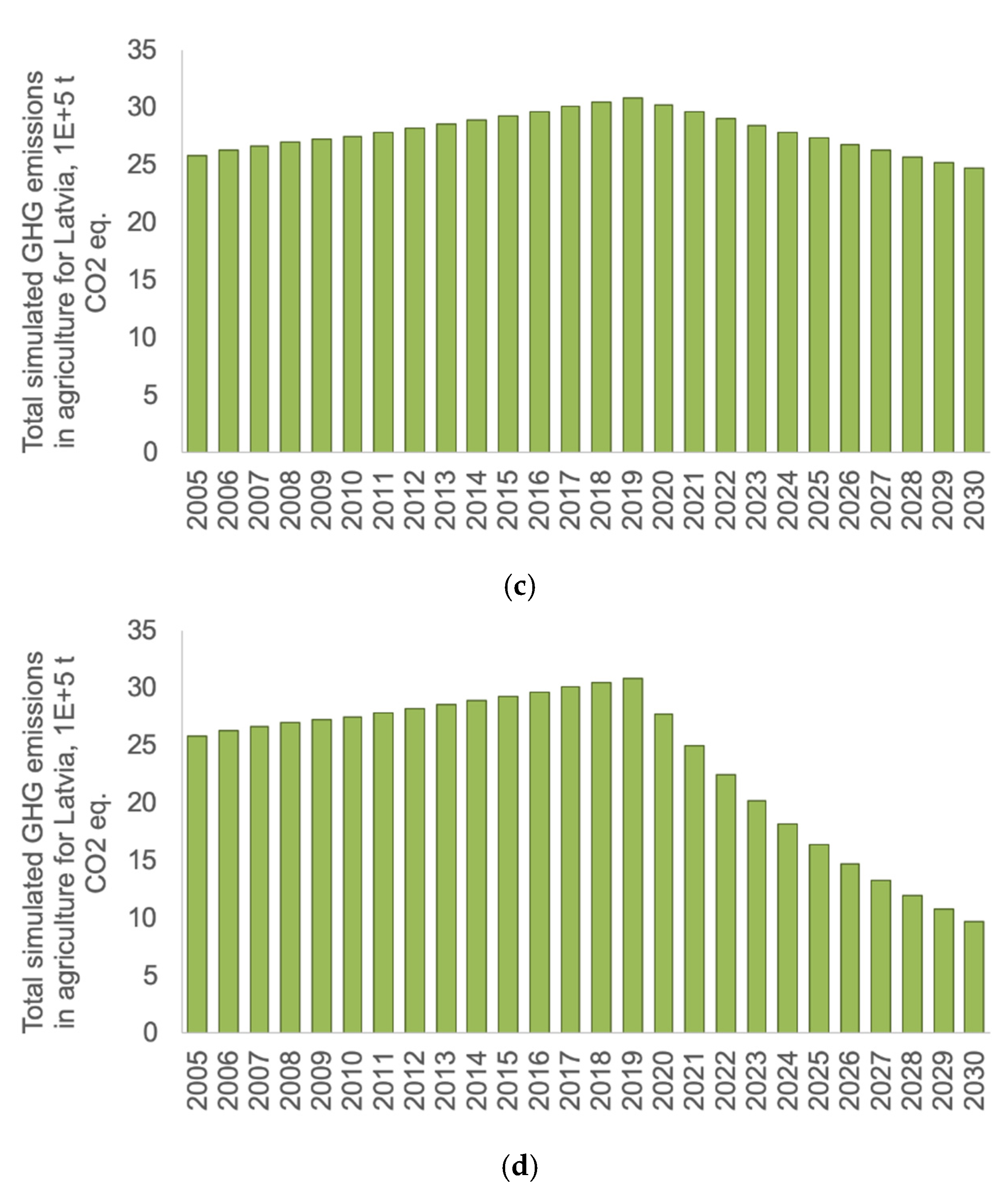
In this case, various different scenarios of the agriculture emission are modelled, such as constant emissions or decreasing emissions; see
Figure 15. As can be seen,
Figure 13a–c depict related trends very precisely. For example, the total emissions from agriculture in Latvia in the year 2030 between scenarios given in
Figure 15a, business as usual or 2% growth of emissions and
Figure 15b, constant emissions after the year 2020 calculated based on BCCM will differ by 4% only. This example shows how hard it is to reach the emission reductions due to accumulation and long perturbation time of these emissions in the atmosphere. In work by Olivié and Peters [
27], the common characteristics and differences between GWP and GTP are discussed. Both methods are designed to be simple tools for comparing impacts to climate from several types of GHG emissions. Both methods refer to the pulse emission of some specific GHG in comparison to the pulse emission of the same quantity of reference CO
2 emissions, while the difference is in the used mathematical model—where GWP is based on comparing the changes in radiative forcing overtime, and GTP on global mean temperature changes over time [
4].
The most significant difference between GWP and GTP is that GTP is an end-point metrics, while GWP is a cumulative measure of climate change. Thus, the value of radiative forcing is of great importance in the analysis of GTP, and more weight is given to climate effects of radiative forcing that come later in the perturbation time of the analyzed pollutants. Thus, for the emissions with a shorter perturbation time, there will be a more significant difference between the results of GWP and GTP results. This theory implies that the GWP assessment gives an overestimation of the short-lived pollutants for the mitigation of climate change. In work by Boucher and Reddy [
30], the difference between black carbon emissions for 100 years perspective in the case of using GTP gave seven times smaller impact than the corresponding GWP assessment. These findings are also in agreement with the work of Shine et al. [
4]. Also, the choice of the time horizon to evaluate the impacts of the emissions is of significant importance. By far, the most common practice is to use a 100-year time horizon, since it is used in the Kyoto Protocol [
27], but there is no scientific justification in using this particular time horizon. The larger the time horizon is chosen, the fewer effects can be attributed to short-lived pollutants [
30]. On the other hand, sustainability cannot be achieved if only long-lived pollutants are accounted and restricted, while short-lived continue to degrade local ecosystems. Therefore, here, both short-term and long-term impacts on sustainability should be assessed and balanced.
Moreover, the choice of the time horizon of 20 years or 100 years or some other time horizon is still not scientifically justified by any concrete evidence [
30]. Thus, the obtained results are also sensitive to the assumed time horizon and can lead to contradicting conclusions.
Our findings are also in agreement with work published by Shimako [
7] and Shimako et al. [
8]. The authors of the research studied the same total amount of emissions but taken with two different emission timing profiles. One emission profile was constant through the simulation, another emission profile peaked in the beginning and then was zero for 4/5 of the simulation. Due to this difference in the emission profiles, the temporal effects of these two emission profiles also differ. In contrast, the total amount of emissions at the end of the simulation was the same for both profiles. In case GWP would be multiplied by the total amount of emissions, the obtained results would be the same for both profiles. This phenomenon is also evident in our findings—the cumulative emissions have different impact profiles when the same amount of total emissions is considered using temporal impacts.
Since the short-lived GHG emissions affect local environments in more apparent patterns, such as effects on air quality, human health, and local ecosystems, in work by Rypdal et al. [
33], it was proposed to regulate short-lived emission in regional policy contexts. The influence of the emissions on local metrics is reviewed in detail in work by Rypdal et al. [
34] and by Levasseur et al. [
6].
Work by Olivié and Peters [
27] also explains that in coupled systems, the temperature changes will also affect the ocean in two ways. Firstly, the absorption of CO
2 directly by the ocean will increase if the temperature will rise. Secondly, ocean circulation patterns will be changing, due to direct effects from increased respiration and photosynthesis or indirectly by changes in precipitation. Also, the authors discuss how various changes in these coupled systems might influence the numerical values used in IRF. Nevertheless, we would like to stress that, in this work, the precise numerical values were not of such high importance as the depiction of overall dynamics and different results that can be obtained using two different methodological approaches.
Also, work by Jardine et al. [
35] shows that various feedbacks exist when CH
4 emissions are analyzed. For example, the global atmospheric lifetime of CH
4 is defined by the amount of atmospheric concentration of CH
4 (CH
4 burden) divided by the amount of annual removal of CH
4 from the atmosphere (CH
4 sink). Thus, increasing the concentration of CH
4 in the atmosphere will lead to longer global atmospheric lifetimes. In work by Holmes [
36], the strength of chemical feedback for CH
4 was analyzed using meteorological, chemical, and emissions factors. The research shows that this feedback depends weakly (likely in the 10% range) on temperature, insolation, water vapour, and emissions of NO. While perturbation time of CH
4 might rise as high as 40% and more, this means that close accounting of the balance in CH
4 is needed in order to have valid assumptions about the time when “constant” values cannot be treated as constants anymore.
To sum up, we believe that both types of emission accounting (the constant GWP values for a 100-year time horizon (GWP100) and the time dynamic GWP values for a 100-year time horizon obtained by using the BCCM) are valuable to use; each has its strength and weaknesses. Thus, we propose to also look on the temporal impacts of emissions, since it might help in designing more precisely targeted policy measures appropriate for the chosen mitigation priorities.
As given in the report by Jardine et al. [
35], CH
4 emissions decay about ten times faster than N
2O, but from the other point of view, policy measures targeting CH
4 reduction will also show the effect on the reduction of climate change ten times faster than measures targeting N
2O. Also, the report by the United Nations Environment Programme and the World Meteorological Organization [
37] shows that the adoption of policies targeting short-lived GHGs would allow reaching climate change mitigation targets with higher confidence. The report also shows that CO
2 reduction measures alone would exceed the set temperature thresholds anyway already in the near term. In contrast, only CH
4 reduction measures would keep the temperature below the threshold in the near term while exceeding the limit later because of the effect of other GHGs. As the opposing argument for stricter control of long-term pollutants is the fact that any technological solution and policy measure will be implemented only for the finite time. Usually, the selected time horizon is much shorter than the consequences of the pollution associated with these technologies.
4. Conclusions
In this paper, two methods for GHG emission accounting were compared. First, using the constant GWP values for a 100-year time horizon (GWP100) and second, the time dynamic GWP values for a 100-year time horizon obtained by using the BCCM that takes into consideration the climate system response to the amount, time and decay rate of the emitted pollutant. The GWP100 values are the default emission metric suggested by the IPCC for the annual emission accounting, and it is considered a relatively simple and easy to use the method. Although no scientific evidence backs the use of GWP100 and, more importantly, GWP100 has “no direct estimation of any climate system responses or direct link to policy goals” (Myhre et al. [
15]; Cherubini et al. [
38]), policymakers widely use the GWP100 values in designing GHG emission mitigation strategies and international agreements, like the Kyoto protocol and Paris agreement.
The results of our study show that the cumulative emissions have different impact profiles when the same amount of total emissions is considered using temporal impacts. The obtained results are also sensitive to the assumed time horizon and can lead to contradicting conclusions. The high sensitivity of the GWP values for the chosen time frame for CH4 and N2O is due to the non-linear nature and different mathematical functions used for approximation of these decay functions. The difference in the average values of GWP for different time horizons can be substantial, and obtained conclusions can be misleading. When using these averages, a situation is also possible when a longer time horizon diminishes the importance of local and relatively short lifetime emissions, such as CH4. For example, the described situation is evident that in the case of N2O emissions, the time frame of 20 or 100 years does not change the applied GWP values so significantly as they change in the case when CH4 is assessed either in 20 or 100 years.
If the impact on the GTP from CH4 is assessed, it can be seen that CH4 shows a more obvious temperature change effect in a shorter run and, in total, contributes to more than half of the temperature change effect created by the agriculture in Latvia.
The BCCM facilitates the selection of the time horizon needed for the specific purpose and expresses the results of policy decisions as to the effect of emissions on the global temperature change potential. The use of GWP100 is still useful and needed as (at least) two purposes of the emission accounting should be separated—one is for the emission inventory, the other is for the policy planning. The inventory is needed to keep track of the annual emission rates and assess the trends and success achieved in the emissions mitigation in the past, and GWP100 is useful for the purpose.
Meanwhile, policy strategies and instruments aim to achieve some desirable behaviour that may effectively govern a system in the future. And the GWP values obtained by using the BCCM would be much more useful for the purpose. Although “countries and the international community have made significant investments in inventory systems’’ [
16] reconsideration and use of other methodology by the policymakers might eventually be less costly than dealing with consequences of climate change and wrong decisions (sub-optimal policies). Application of the BCCM would facilitate finding more efficient mitigation options for various pollutants, analyze multiple parts of the climate response system at a specific time in the future (amount of particular pollutants, temperature change potential), or analyze different solutions for reaching the emission mitigation targets at regional, national, or global levels.


