1. Introduction
A multi-disciplinary optimization (MDO) design, which is among the latest and most active fields in the current research on complex system optimization design, is mainly used in specializations such as aerospace and torpedo missile design. The research on MDO in fluid machinery is mainly focused on the optimization design of turbine and wind turbine blades. However, pumps are classified as general machinery with varied applications [
1,
2,
3,
4,
5]. The axial-flow pump impeller is the core and most important flow component of a pump device. The result of the design directly determines the comprehensive effects of the pump device and the entire pumping station. In recent years, approximately half of the axial-flow pump impellers produced annually have been used to replace scrapped products caused by blade problems [
6]. To improve the comprehensive performance of axial-flow pump impellers, a multi-disciplinary optimization design of an axial-flow pump impeller should be implemented.
MDO is mainly used in some large-scale systems engineering. Sun et al. [
7] used the MDO platform to focus on integral solid propellant ramjet supersonic cruise vehicles and constructed two MDO frameworks through discipline codes. Thus, the optimization of the detailed parameters and high fidelity were achieved. Chen X et al. [
8] adopted MDO by introducing the multi-disciplinary feasible architecture and gradient-based optimization algorithm, which further improved the efficiency of gradient calculation. The optimized design was more energy-saving than the initial design. Xu HW et al. [
9] dealt with time-varying uncertainty by proposing a multi-disciplinary robust design optimization method based on time-varying sensitivity analysis through a multi-disciplinary optimization design. MDO provides a good solution in the fields of launch vehicle design optimization, hard rock tunnel boring machine performance design optimization, and all-electric GEO satellite design optimization [
10,
11,
12,
13,
14]. The MOD technology has incomparable advantages in solving the optimization design problem of large-scale complex systems engineering.
The optimal design of a pump is based on the design theory and method of pumps, which uses optimal design theory to achieve superior comprehensive performance [
15]. At present, optimization methods for pumps mainly include those based on simplified model prediction and accurate model analysis. To improve the efficiency of a centrifugal pump, Wang WJ et al. [
16] and Pei J et al. [
17] optimized the impeller and guide vane, thereby obtaining a highly efficient hydraulic model. Miao F et al. [
18] proposed a multi-objective optimization of the impeller shape of an axial-flow pump based on the modified particle swarm optimization (MPSO) algorithm. This novel algorithm was successfully applied for the optimization of axial-flow pump impeller shape designs by comparing the results of the MPSO and Computational Fluid Dynamics (CFD) simulation results. Yun JE [
19] studied the impact loss at the inlet of rotor blades and obtained the optimal design of a blade shape by numerical analysis and optimization. Some studies [
20,
21] have adopted optimization design methods to achieve improved cavitation and good hydraulic performance of axial-flow pumps. Numerous studies have shown that the numerical simulation method has become the most important research method in the field of pumps. However, the majority of these studies have used a single subject optimization method to obtain the design result of pumps, in which the hydraulic performance and structural strength were optimized separately.
Only a few studies have been conducted on the fluid–structure coupling of pumps. These studies used the fluid–structure coupling analysis method based on the MDO platform to optimize the blades of pumps [
22,
23]. Tong YF et al. [
24] implemented a multi-disciplinary energy-saving optimization design of bridge cranes and adopted the finite element analysis and multi-disciplinary optimization technology to reduce the total quality and energy-saving design of cranes. However, these studies have yet to achieve the degree of coordinated design optimization of hydraulic performance and structural strength.
The current study draws on the relevant research methods in the aforementioned fields to adopt an MDO design method for large axial-flow pump blades. At present, the rapid development of computational fluid and structural mechanics has resulted in numerous and successful research in the field of hydraulic performance and structural performance of axial-flow pump impellers. However, the traditional single-discipline optimization analysis method disregards the interaction and mutually affects between the hydraulic and structural designs. The method also fails to achieve a real coordinated design, which does not consider the reliability and accuracy of the optimized design results. To further improve the overall performance of pumps in axial-flow pump impeller optimization designs, the theory and method of multi-disciplinary design optimization of axial-flow pumps were applied in this research. This study focuses on the two disciplines of hydraulics and structure. Therefore, the MDO problem in this research can be presented as follows: considering the blade quality and efficiency of the design condition as objective functions; using the head of small flow (i.e., flow under the highest operating head), efficiency of small flow, maximum stress value, and maximum deformation value of small flow as constraints; and ensuring that the blade head of the design conditions remains unchanged or varies in a small range.
2. Numerical Calculation
2.1. Governing Equations
The solution of the fluid–structure interaction problem should consider the flow and structure fields and the data transfer between them. To considerably study this interaction, the current research used the calculation method of unidirectional fluid–solid coupling based on the system coupling module of the Ansys Workbench platform. First, the calculation of the fluid domain is performed. Second, information on the fluid domain is transmitted to the structural field by the fluid–solid coupling interface. Lastly, finite element structure analysis is performed.
In the flow field calculation, three-dimensional (3D) Reynolds-averaged N–S equations are used to solve the turbulent flow in the impeller of the axial-flow pump. By solving the equation, the fluid information of the discretized time and space flow field is obtained. The performance shows that the parameters can obtain the flow field flow characteristics. The basic control equations are as follows:
where
v is the inflow velocity,
p is the flow field pressure,
ρ is the fluid density,
μ is the fluid dynamic viscosity, and the subscripts
i and
j are the x- and y-coordinates, respectively.
The numerical simulation adopted the renormalization group(RNG)
k-ε turbulence model. When water flows through the blade passage of the axial-flow pump impeller, it will produce a higher strain rate and larger bending streamline. The RNG
k-ε model adopts a statistical technique called renormalization grouping to correct the turbulence viscosity by considering the condition of rotation and swirl. The RNG
k-ε turbulence model has better analysis ability than other turbulence models in the internal flow field calculation process of axial-flow pumps. The governing equations are as follows:
where
Gk represents the generation of turbulence kinetic energy caused by the mean velocity gradients. The quantities
αk and
αε are the inverse effective Prandtl numbers for
k and
ε.
C1ε = 1.42,
C2ε = 1.68.
μeff is the effective viscosity accounting for turbulence.
k is turbulence energy.
ε is dissipation rate of turbulent kinetic energy.
The structural calculation used the finite element method to analyze the structural field of the axial-flow pump blade. The dynamic equation of the axial-flow pump blade under hydrodynamic action is defined as follows:
where [
M] is the structural mass matrix, [
C] is the structural damping matrix, [
K] is the structural stiffness matrix, (
x) is the structural displacement,
is the structural velocity,
is the structural acceleration, and {
F} represents the flow field force of the structure under a fluid–solid coupling.
When the static calculation of axial-flow pumps blade is performed through fluid–solid coupling, the fluid and solid systems are included in such a calculation. On the coupling surface, the velocity and stress continuous equations should be satisfied. The water pressure on the blade surface under a certain operating condition of pumps can be approximated and is constant with time. That is, the time-related quantity is disregarded. Thus, the relationship can be simplified as follows:
where
and [
B] is the strain matrix.
The stress requirement for the MDO design of axial-flow pumps is the most important. The stress distribution of blades under the design conditions is unnecessary because the general pumping station project focuses on the highest head. The most important aspect in terms of hydraulic performance is the efficiency of the design conditions. The highest operating head conditions focus on safe operations. The practical application requirements of pump stations and the corresponding flow given under the highest operation head of these stations indicate the calculation of stress distribution by using the head as a constraint under this flow. In energy saving and emission-reduction environments, blade quality is regarded as the goal of structural optimization design. Therefore, the MDO problem in this research can be presented as follows: considering the blade quality and efficiency of the design condition as objective functions; using the head of small flow (i.e., flow under the highest operating head), efficiency of small flow, and maximum stress and maximum deformation values of small flow as constraints; and ensuring that the blade head of the design conditions remains unchanged or varies in a small range. Under these conditions, the impeller of the axial-flow pump undergoes multi-constraint, multi-objective, multi-modality, and multi-disciplinary optimization.
2.2. Parameterized Model
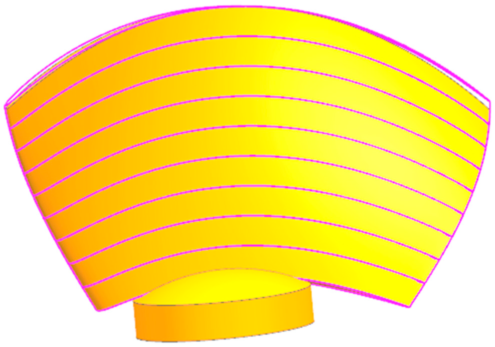
A blade modeling program written in MATLAB based on the Zhukovsky airfoil can generate blade curve files for Turbo-Grid and UG. In this manner, the 3D model of the fluid and 3D model of the blade structure can be established conveniently. The flow–solid coupling calculation analysis of axial-flow pumps is only for the impeller. Thus, the analysis only involves the calculation of the single channel flow field to save calculation time and improve calculation efficiency in the flow field analysis. Structural calculations consider the single blade in the corresponding coordinate quadrant. The majority of the axial-flow pumps in actual pumping stations are fully regulated vane pumps. To fit the actual situation, a 3D modeling of the model impeller round shank is performed instead of a 3D hub shape, with the inner surface of the round shank being a fixed end. The 3D model of the blade structure is shown in
Figure 1.
2.3. Grid and Load
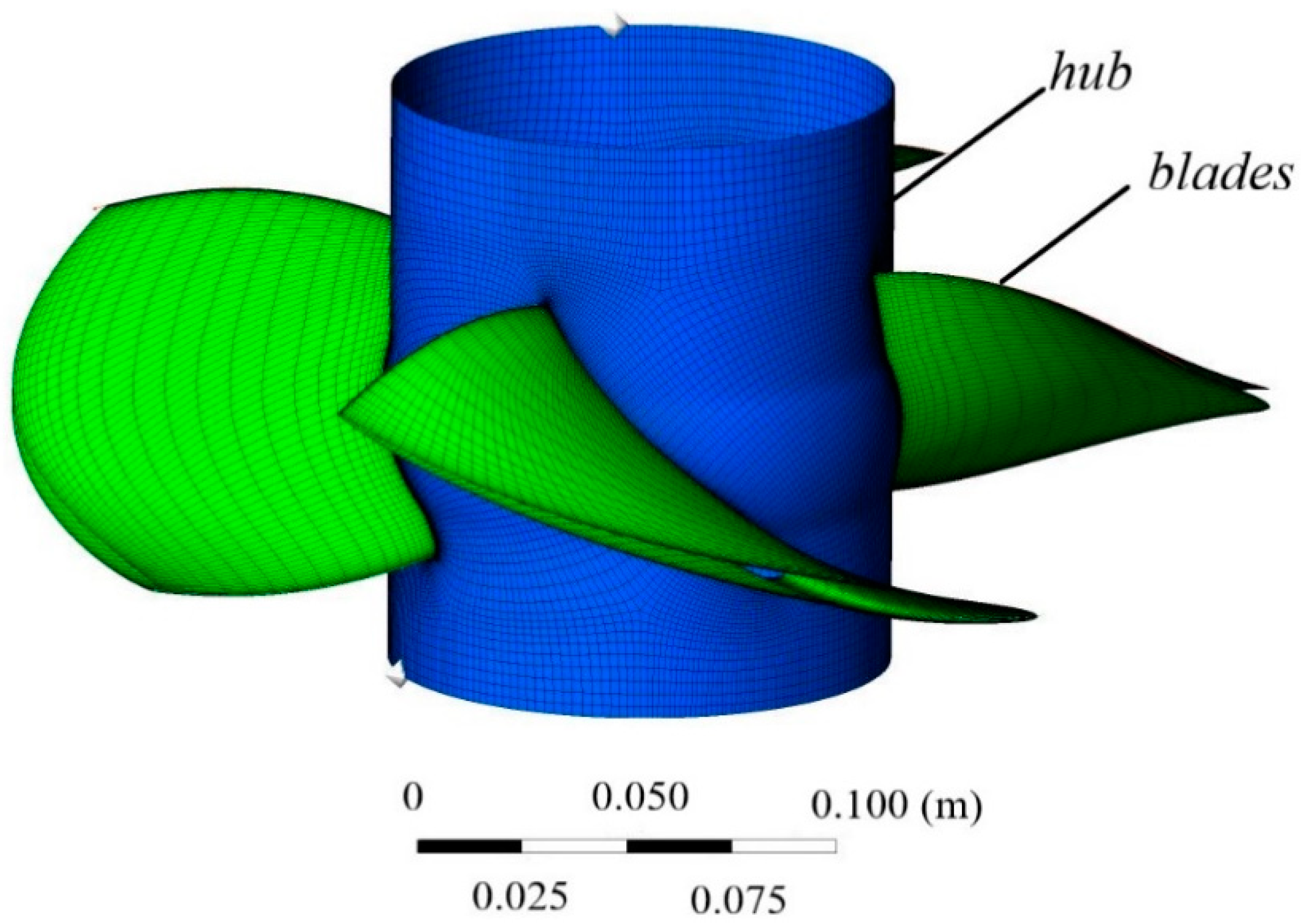
The fluid domain calculation model is mainly for the impeller of axial-flow pumps. In this study, the nominal specific speed of the axial-flow impeller ns is 750, design flow Q is 360 L/s, design head H is 7.0 m, rotating speed n is 1450 r/min, and the blade tip unilateral gap is 0.15 mm. The diameter of the impeller is 300 mm. The number of impeller blades is four. The impeller is modeled by using Turbo-Grid according to the 3D coordinate data points. The axial-flow pump impeller is the computational domain. The inlet and outlet of the computational domain are respectively set as the total pressure inlet and the flow outlet. No-slip conditions are used for all the walls.
The structural grid of the axial-flow impeller is meshed by the software of Turbo-Grid. The quality of the grid is good and can meet orthogonal requirement. The grid of the impeller is shown in
Figure 2.
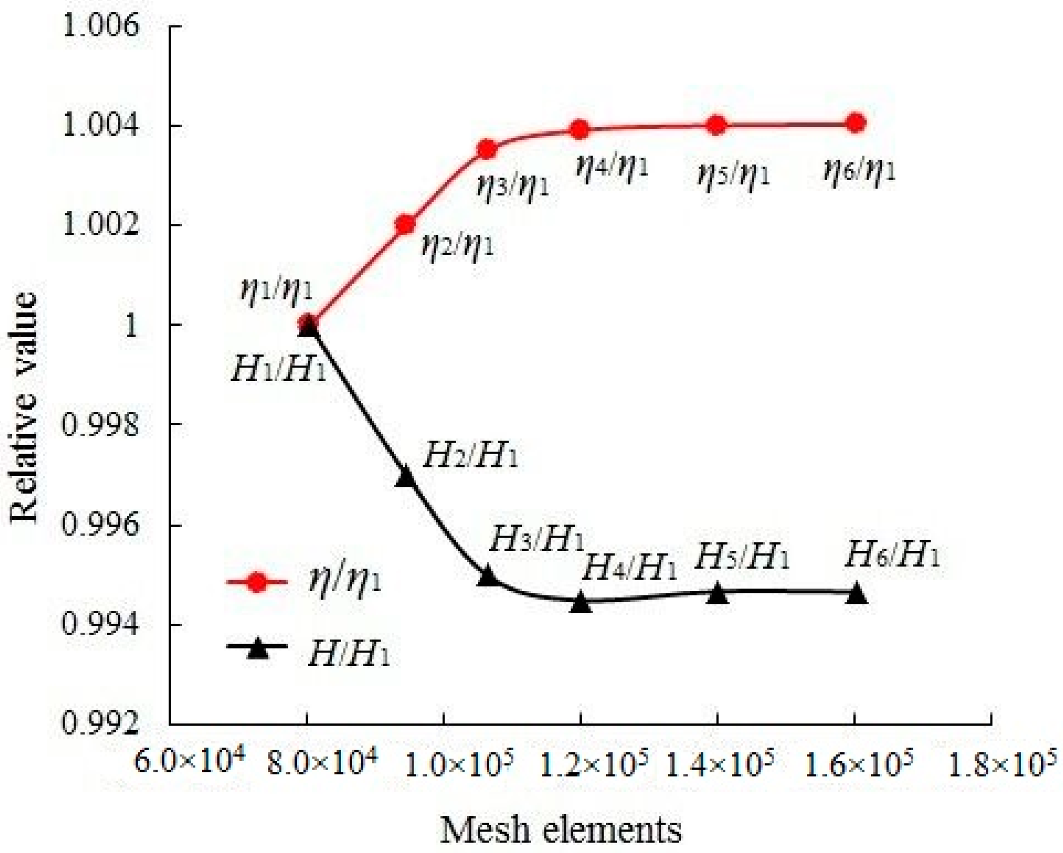
In the mesh elements ranging from 8.0 × 10
4 to 1.6 × 10
5, six sets of single channel grids of the impeller are used to do the grid independence analysis. Numerical calculation results of the head and efficiency of the impeller reveal a small difference when the grid elements are up to 1.21 × 10
5 (
Figure 3). Therefore, 121,527 is selected as the number of single channel computational mesh elements for numerical simulation in this study.
Bernoulli energy equations were adopted to calculate the head of axial-flow pump. The head of the pump is shown as follows:
where
H1 is the inlet water level,
H2 is the outlet water level (m),
s1 is the inlet section area,
s2 is the outlet section area (m
2),
u1 is flow velocity of inlet section,
u2 is flow velocity of outlet section (m/s),
ut1 is the normal component velocity of inlet section,
ut2 is the normal component velocity of outlet section (m/s),
P1 is static pressure of inlet section, and
P2 is static pressure of outlet section (Pa).
The efficiency of the axial-flow pump is shown as follows:
where
Tp is torque of the blade (N·m), and
ω is the angular velocity of the impeller (rad/s).
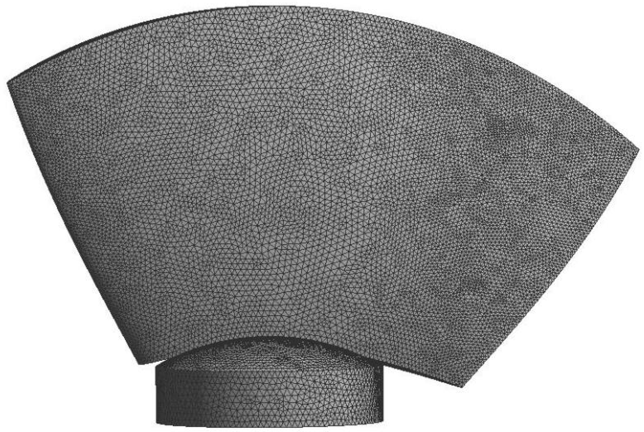
According to the actual situation of the blade structure, the 3D solid model is imported into the Design Modeler module of the Workbench platform to set the properties of the model material to structural steel.
The material property parameters of the axial-flow pump blade are as follows: modulus of elasticity E = 2.0 × l0
11 Pa, Poisson’s ratio
μ = 0.3, and density
ρ = 7850 kg/m
3. The diameter and thickness of the round shank are 60 mm and 12.5 mm, respectively. The solid grid model is divided in the mesh module of a model that uses unstructured grids. The number of grids of a single blade is around approximately 120,000. The grid model is shown in
Figure 4.
This study calculated the stress distribution of a pump blade under inertial and pressure loads. Inertial load is the centrifugal force received by the pump. The pump’s rate of speed is n = 1450 r/min. The pressure load is the water pressure. In the structural analysis, the influence of bearing load and bolt load on the stress distribution is disregarded for convenience of calculation.
2.4. Model Test Verification
A field performance test of the initial scheme was carried out on an axial-flow pump model test bench in China. The impeller of the axial-flow pump was machined with copper material according to design results of the initial scheme. The rotating speed of the impeller was 1450 r/min, and the diameter of the impeller was 300 mm. The number of the blades was four. The impeller of the axial-flow pump is shown in
Figure 5a. According to the hydraulic industry standard of the pump model test of China, the model test of the axial-flow pump section includes impeller, guide vane, inlet pipe and outlet pipe, etc. The guide vane adopts the matching design guide vane. The pump installation is shown in
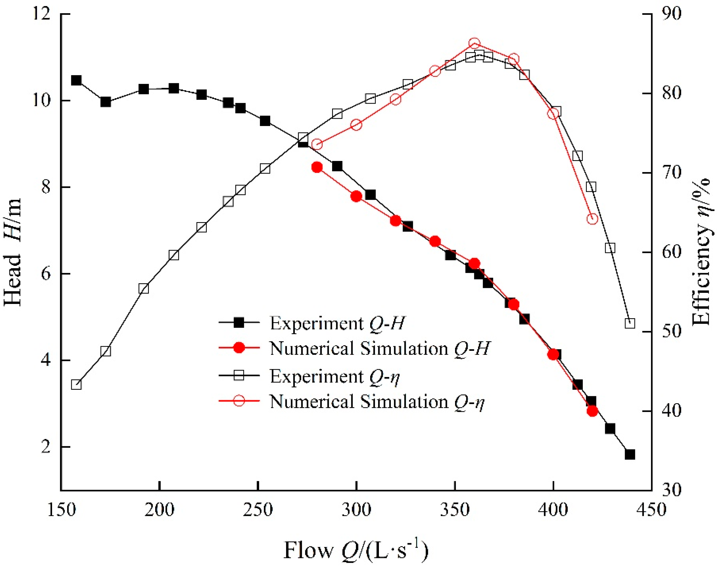
Figure 5b. The comparison of numerical simulation and model test is shown in
Figure 6. The predicted performance curve of numerical simulation is consistent with the experimental curve. The curves have a good agreement, and the error of each point is less than 3%. The results show that the numerical simulation of the axial-flow pump is accurate and reliable.
3. Analysis of Design of Experiment
The optimal Latin hypercube method was selected for the calculation of the sample points in the flow–solid coupling calculation of the axial-flow pump. This method allows many more points and more combinations to be studied for each factor. Experiment points are spread evenly, allowing higher order effects to be captured. The engineer has total freedom in selecting the number of designs to run as long as it is greater than the number of factors. The optimal Latin hypercube method is based on the random Latin hypercube method to improve the uniformity. The level selection of the factors is regulated by the corresponding algorithm, so that the selected sample points have better space filling and more uniform distribution in the whole design space.
The design variables included four design parameters: cascade density, airfoil placement angle, airfoil arch ratio, and airfoil thickness ratio. Airfoil selects the Zhukovsky airfoil structure used in the flushing angle research. All parametric modeling works were implemented in MATLAB. The 3D coordinate data of the blade section were generated using MATLAB, while the 3D solid models were built in Turbo-Grid and UG. To save calculation time and improve efficiency, the 3D shape of the entire blade was controlled using the minimum design variables. By using the equal strength design method, the cascade density of 10 sections can be controlled by two design variables: cascade density multiple of the blade tip and cascade density multiple of the blade root. The third-order B-spline curve control can reduce the airfoil angle data of 10 sections to only three variables: airfoil angle of the hub, rim, and middle section. The maximum camber and maximum thickness of the 10 sections are linear from hub to rim. Therefore, each parameter is only controlled by two variables of the hub and the rim, which successfully reduces 40 design variables to nine design variables. The initial value and range of the nine design variables are as follows:
where
x1 is the cascade density of the blade tips,
x2 is the cascade density multiple of the blade root,
x3 is the airfoil angle of the hub (°),
x4 is the airfoil angle of the rim (°),
x5 is the airfoil angle of the middle section (°),
x6 is the maximum camber of the hub (mm),
x7 is the maximum camber of the rim (mm),
x8 is the maximum thickness of the hub (mm), and
x9 is the maximum thickness of the rim (mm).
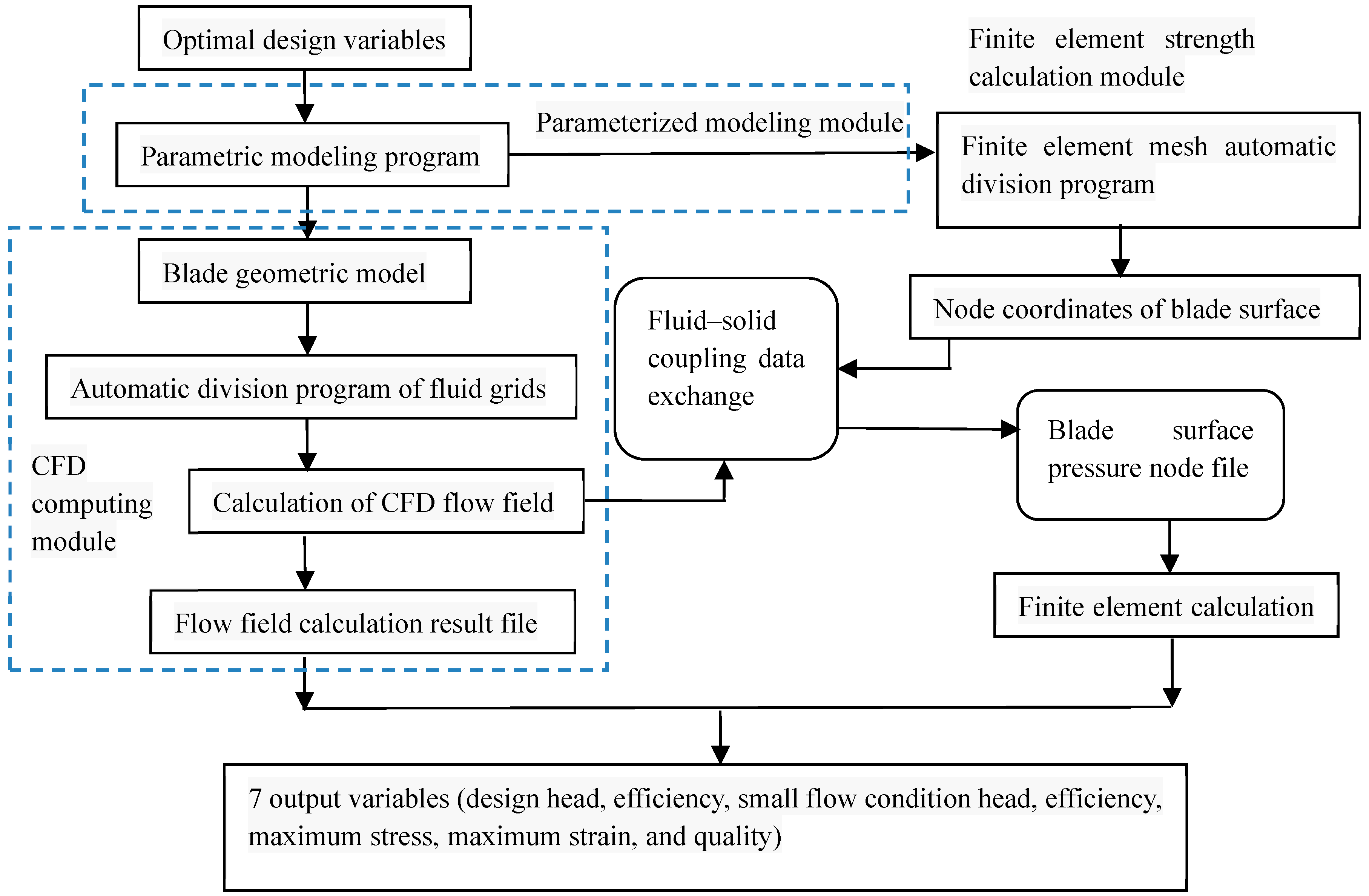
Within the range of the design variables, 80 sample points were generated using an optimized Latin hypercube method. A complete fluid–solid coupling calculation is required for each set of sample points. Each fluid–solid coupling calculation requires a complete set of processes including 3D modeling of fluid and structure, mesh division, and flow field and finite element calculation. Each flow–solid coupling calculation process is shown in
Figure 7.
According to the optimization requirements, the structural parameters, including mass, maximum stress, and maximum strain, should be calculated. Hydraulic parameters include the head and the efficiency under design conditions and small flow conditions. The design and small flow conditions are 360 L/s and 240 L/s, respectively.
Table 1 shows the calculation results of the 80 sample points.
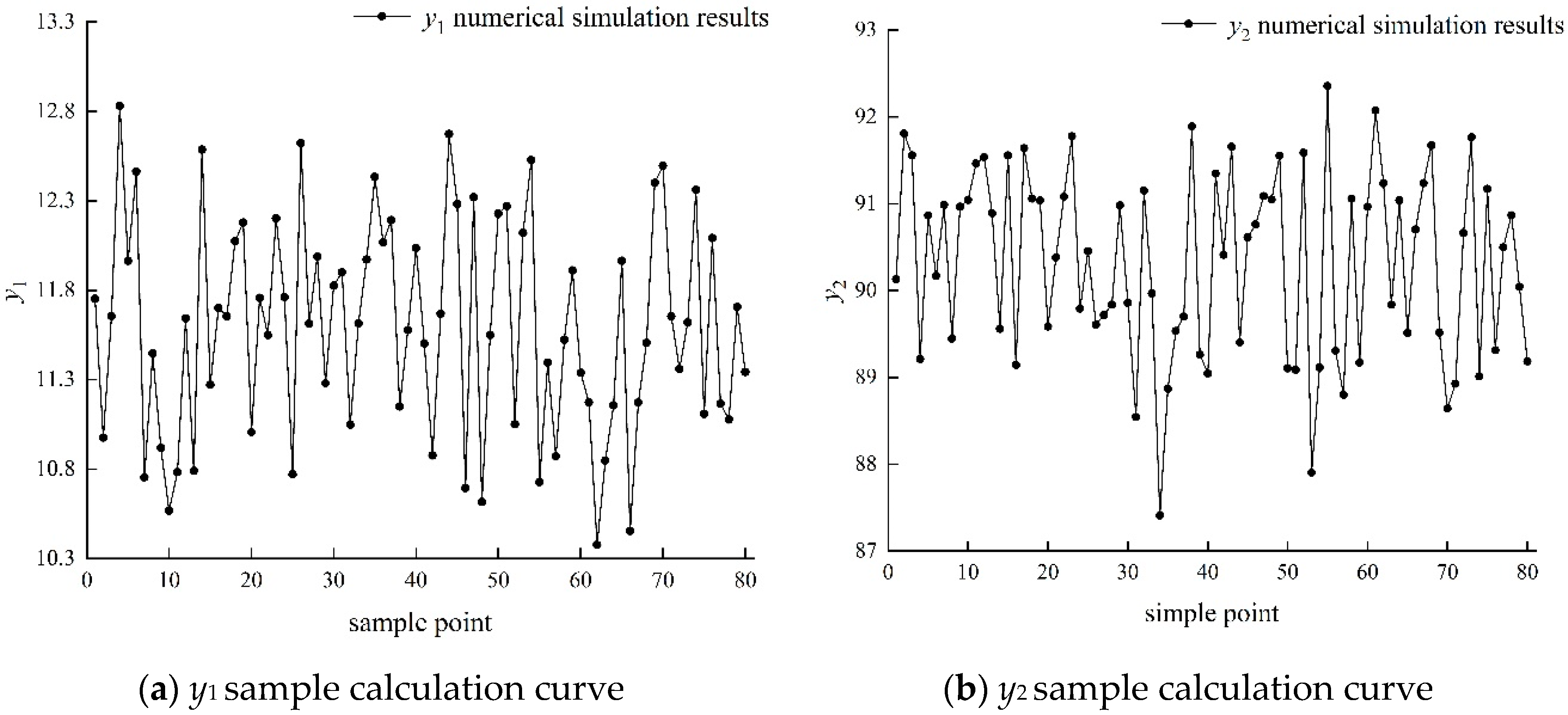
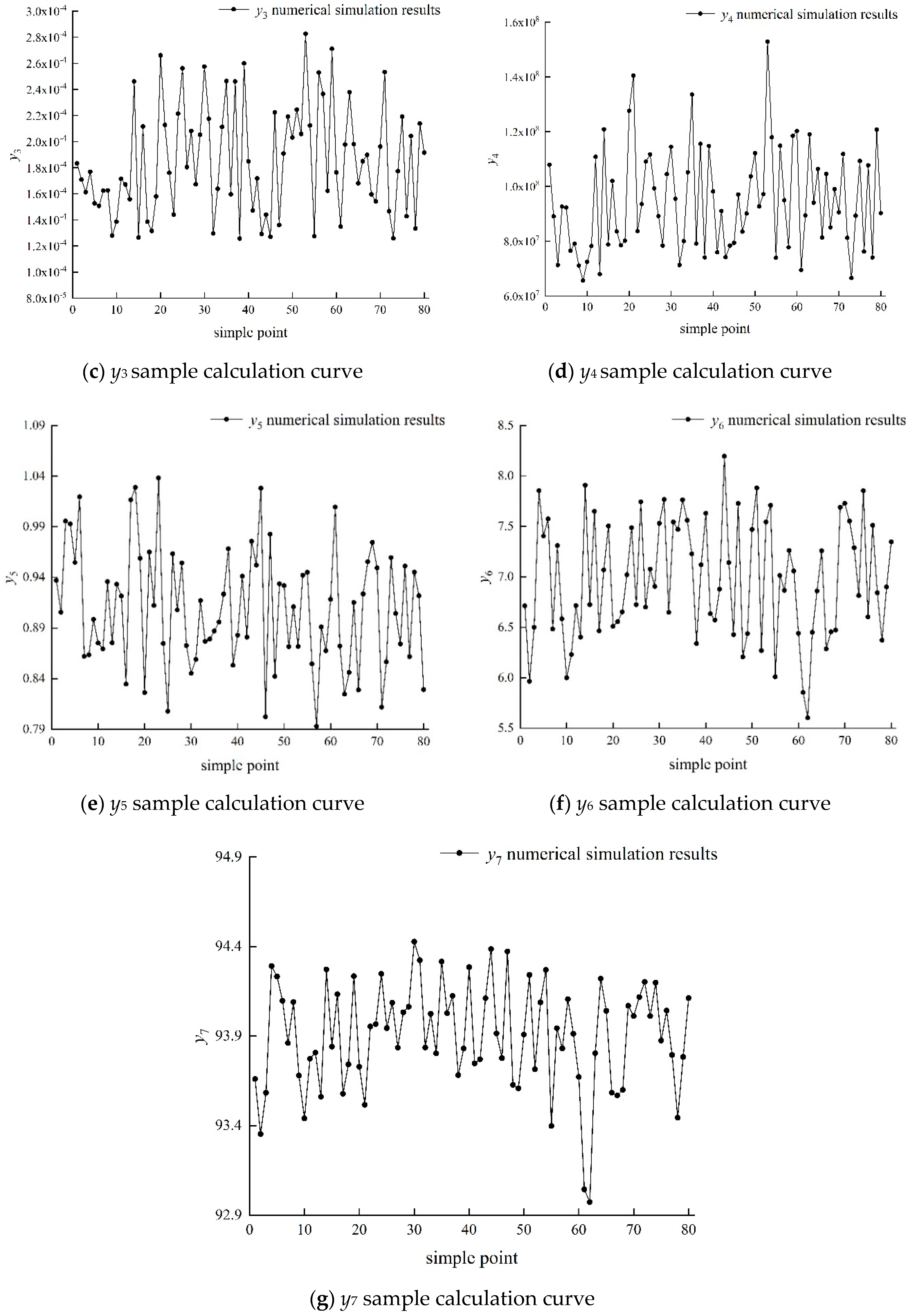
The calculation results of hydraulic performance and structural performance of the axial-flow pump were obtained according to 80 different blade design schemes. In the calculation results of 80 groups of samples, the minimum value of the head was 10.38 m and the maximum value was 12.83 m under the small flow condition (
Figure 8a). The lowest value of the pump efficiency was 87.41%, and the highest value was 92.36% under the small flow condition (
Figure 8b). Under the small flow condition, the maximum deformation of the pump blade was in the range of 0.126~0.287 mm (
Figure 8c). Under the small flow condition, the maximum stress of the pump blade was in the range of 65.6~152.9 MPa (
Figure 8d). When the axial-flow pump was operated under small flow conditions, the pump head was relatively high, and the blades in this operating area were most vulnerable to structural damage. Therefore, it is necessary to consider structural deformation and structural stress under small flow condition when doing structural optimization design. The minimum mass value of the single axial-flow pump blade under different design schemes was 0.79 kg, and the maximum value was 1.04 kg (
Figure 8e). Under the design condition, the minimum value of the head was 5.60 m, and the maximum value was 8.19 m (
Figure 8f). Under design condition, the minimum value of the pump efficiency was 92.97%, and the highest value was 94.43% (
Figure 8g). The head and efficiency of the axial-flow pump under design condition are very important evaluation parameters for the design of the axial-flow pump. In order to ensure that the specific speed of the pump is constant, the head under the design condition should be kept basically unchanged, and at the same time, the efficiency is expected to be higher. The difference between the calculation results of the different sample points is relatively large, particularly the structural performance (
Figure 8). The maximum calculation results of the maximum stress and deformation value were more than twice the minimum value. This result shows that the change of the design parameters has immense influence on the structural performance of pump.
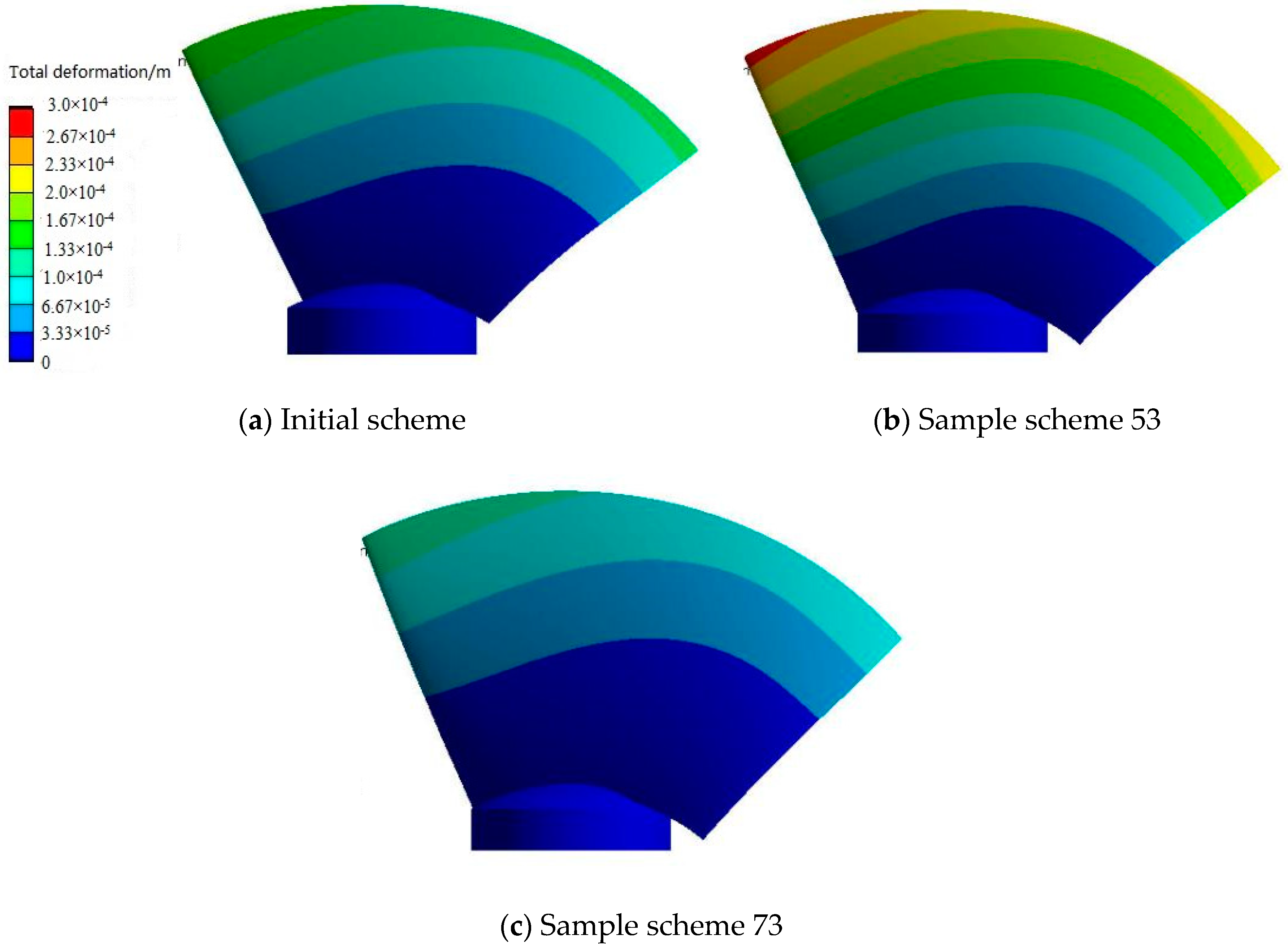
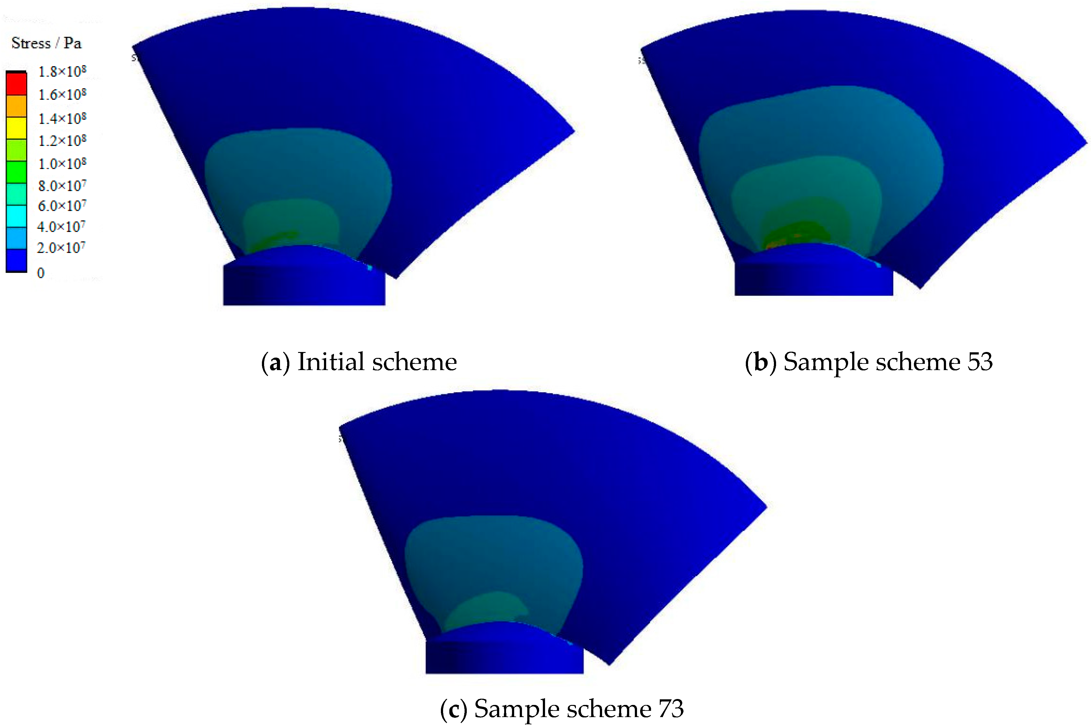
The three typical conditions of stress and strain distribution are shown in
Figure 9 and
Figure 10.
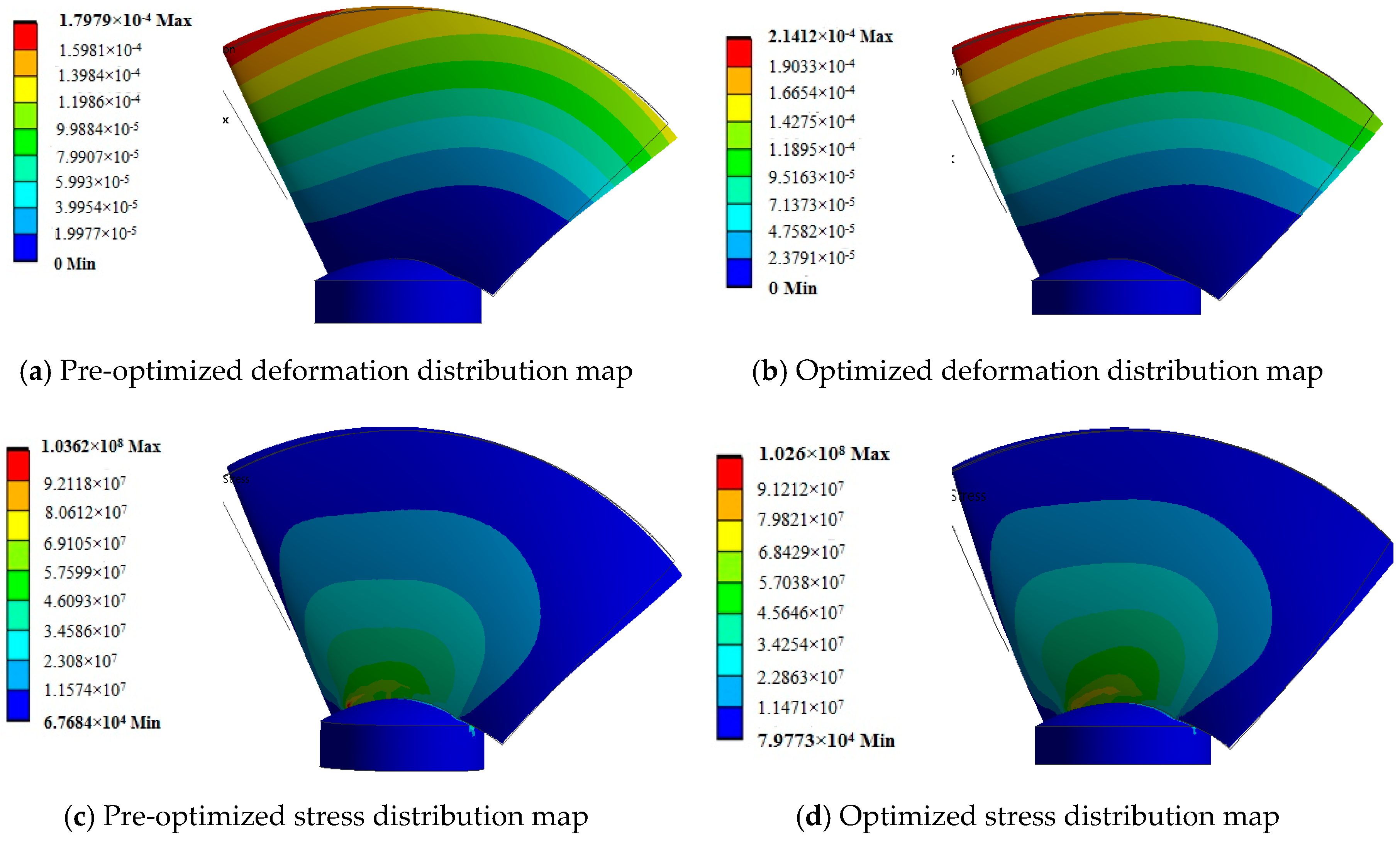
The structural performance calculation results of sample points 73 and 53 were taken out to analyze their structural characteristics because the structural performance of sample points 73 and 53 were the maximum and minimum values respectively in the whole sample. Evidently, the maximum deformation position of the blade of the axial-flow pump was near the edge of the blade inlet section. The maximum stress position was near the hub of the blade. The maximum stress and maximum deformation position and distribution trend corresponding to the different design parameters were consistent. However, the maximum deformation and maximum stress values differed substantially. The solid line in the graph indicates the position of the blade when it was not subjected to external stress. The cloud image shows the position after deformation. The deformation direction of the blade was the same. The deformation was found toward the inlet direction of the impeller; the closer the rim, the more substantial the deformation was.
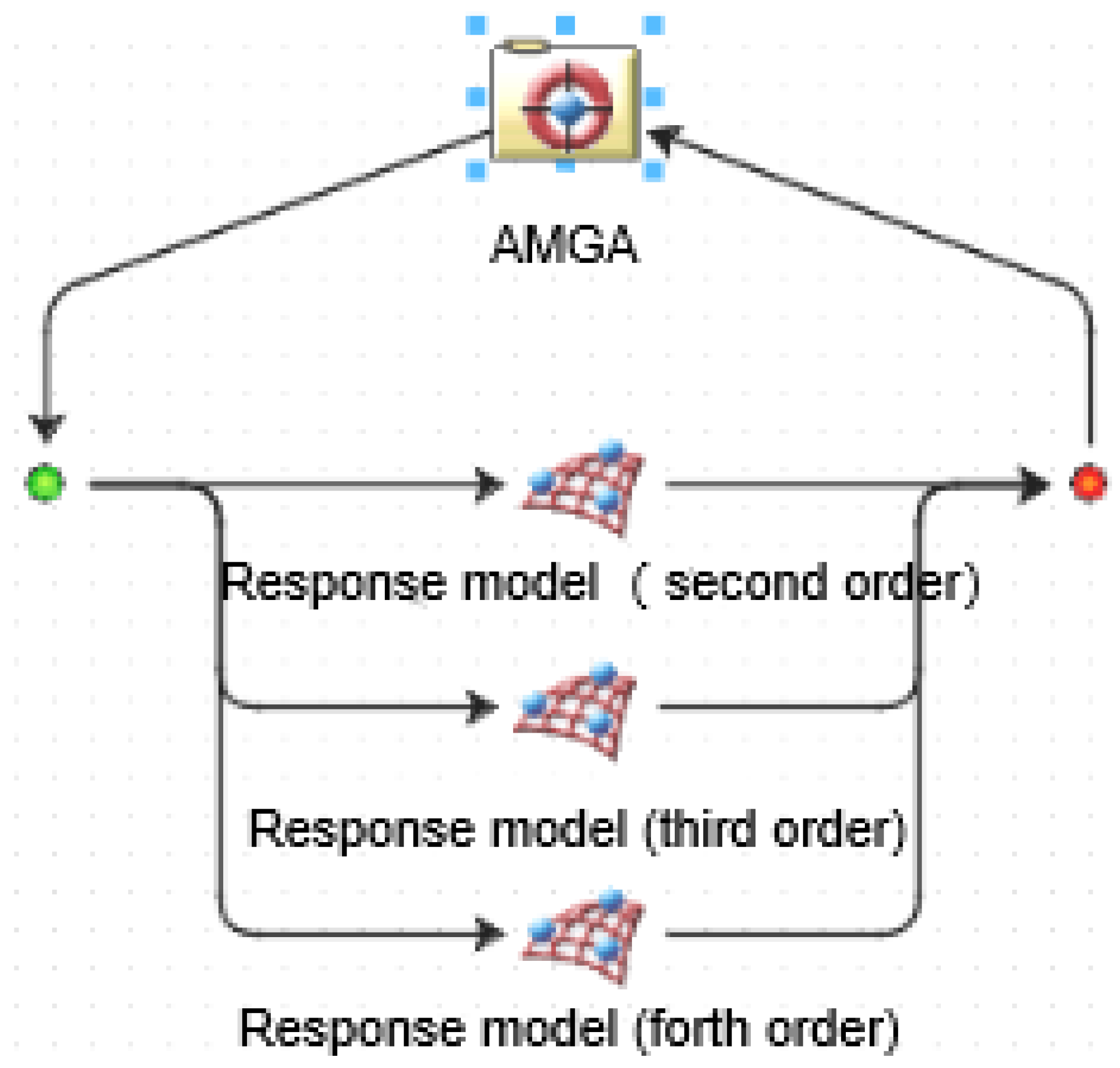
4. Approximation Models
Approximation models are methods of approximating a set of input variables (i.e., independent variables) and output variables (i.e., response variables) through a mathematical model. The approximate model uses the following equation to describe the relationship between the input variable and output response:
where
is the response to the actual value, which is an unknown function;
is a response to the approximation, which is a known polynomial; and
is the random error between the approximation and actual value, which typically follows the standard normal distribution of
.
An approximate model structure was constructed and aimed at the 80 sample points of the axial-flow pump multi-disciplinary optimization design. R2 is a regression coefficient that characterizes the correlation between the predicted and actual values. When R2 is equal to 1, the predicted value of each sample point is the best fit with the actual value; the closer the R2 coefficient of the approximate model to 1, the closer the approximate model to the real solution. The R2 coefficients of the different approximation models are listed as follows.
R-squared can be used to analyze the degree of consistency between the approximate model and the sample points. An R-squared value of 1.00 indicates that the approximate model has high reliability. The credibility is low when the value of R-squared is less than the set acceptance level of 0.8. The approximate models were established by means of RSM method, neural network method, and Kriging method. The R-squared value of
Table 2 displayed in red is closest to 1. It shows that the approximate model displayed in red is the most ideal scheme, and it has high reliability.
Table 2 shows that the Kriging model cannot fit the approximate model data of the two responses—the largest deformation and maximum stress values and the effect is not good when fitting other responses. Hence, the Kriging model was not used in this study. When using neural network models to construct approximate models, the radial and elliptical basis models have minimal effect on the fitting results. These models only have a good fitting effect on part of the responses. The response surface model has a superior fitting effect.
Table 2 shows that the more complex the response of the maximum stress value, the higher the order and the better the fitting effect, which was not the case in the other responses, particularly in the quality response. The fitting quality of the fourth-order response surface model decreases substantially. This study used the second-order response surface method to construct an approximate model of the small flow rate efficiency and quality, in accordance with the comparative results of the fitting effect. The third-order response surface method was used to construct an approximate model of the small flow head and the design condition head. The fourth-order response surface method was used to construct an approximate model of the small flow maximum deformation, maximum stress, and design efficiency.
6. Conclusions
This study applied the theory and method of multi-disciplinary design optimization of the axial-flow pump to further improve the overall performance of the axial-flow pump impeller optimization design in this research. The MDO problem in this research was addressed can be concluded as follows: considering the blade quality and efficiency of design condition as an objective function; using the head of the small flow, efficiency of the small flow, maximum stress value, and maximum deformation value of the small flow as constraints; and ensuring that the blade head of the design conditions remains unchanged or varies in a small range. According to the range of the design variables, 80 sample points were generated using an optimized Latin hypercube method. Thereafter, the response surface method was used to build the approximate model according to the sample points. Lastly, the optimal design of axial-flow pump impeller was carried out by the approximate model, and the impeller satisfying the constraint conditions was obtained. The following results were obtained through calculation and analysis.
- (1)
From the 80 sample points, the difference between the calculation results of the different sample points was relatively large, particularly for the structural performance. The maximum calculation results of the maximum stress and deformation value were over twice the minimum value, which shows that the change of design parameters had a substantial influence on the structural performance of the pump. The response surface model had a superior fitting effect. This study used the second-order response surface method to construct the approximate model of the small flow rate efficiency and quality, in accordance with the comparative results of the fitting effect. The third-order response surface method was used to construct the approximate model of the small flow and design condition head. The fourth-order response surface method was used to construct the approximate model of the small flow maximum deformation, maximum stress, and design efficiency.
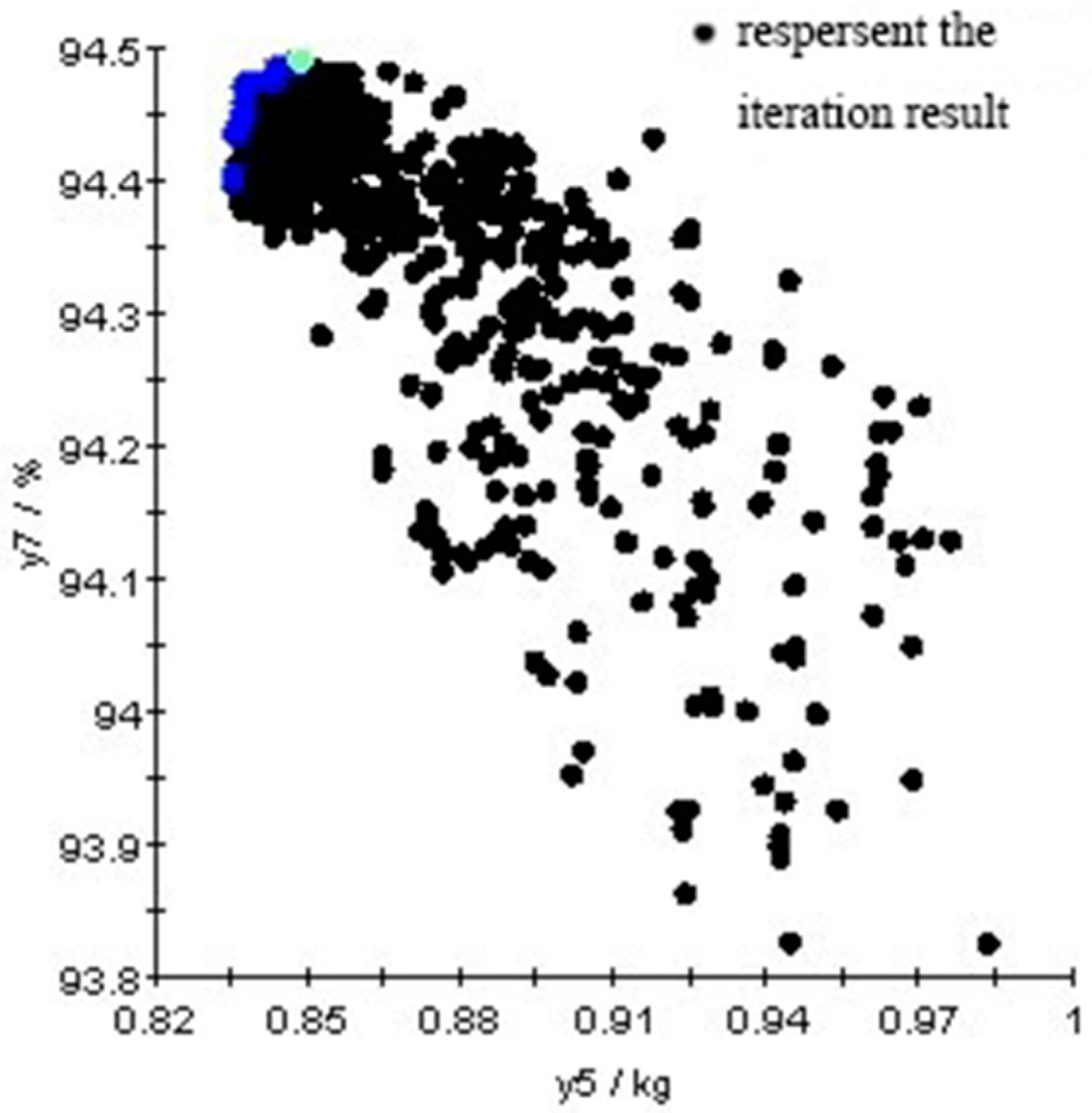
- (2)
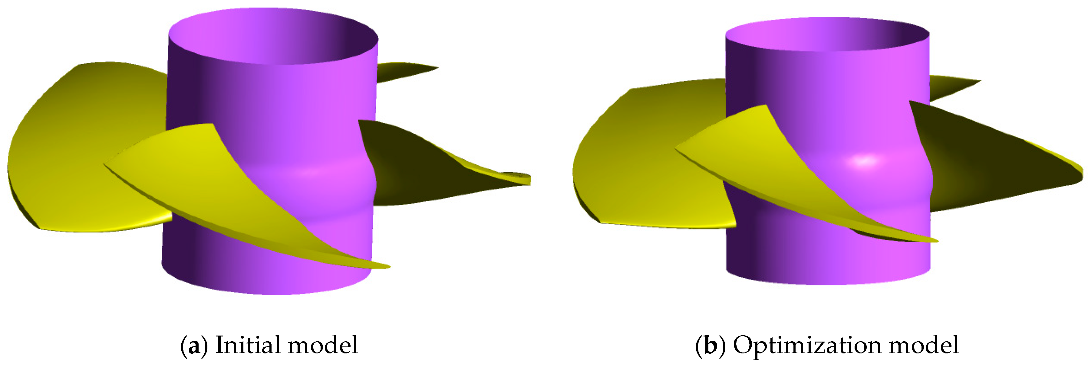
For the construction of the approximate model of the MDO design, the fitting effect of the response surface approximate model was better than that of the other approximate models. The results of the MDO design of the impeller are as follows: the quality decreased from 0.947 kg to 0.848 kg; the decline reached 10.47%, whereas the design efficiency increased from 93.91% to 94.49%; the increase was 0.61%; and the optimization effect was obvious. In addition, the errors of the other responses were below 0.5%, except for the maximum stress value error. The approximate model has high accuracy and the analysis results are reliable.
As we all know, the impeller of the axial-flow pump is the core and most important flow part in the pump station. The design quality of the impeller directly determines the overall efficiency of the pump device and even the pumping station. With the increasingly complex operational requirements, the pump design has to meet higher design requirements [
25,
26,
27]. A multi-disciplinary design optimization [
28] method can combine hydraulic design and structural design, so that it can get the optimized impeller to match the complex operating conditions. This present study solved some key technical problems in the MDO process of the axial-flow impeller. However, in addition to the mass of the blade, how to combine vibration characteristics, hydraulic noise, and materials to carry out multi-disciplinary optimization design is the main content of future studies.


