Abstract
The identification of high risk regions is an important aim of risk-based inspections (RBIs) in pipeline networks. As the most vital part of risk-based inspections, risk assessment makes a significant contribution to achieving this aim. Accurate assessment can target high risk inspected regions so that limited resources can mitigate considerable risks in the face of increased spatial distribution of a pipeline network. However, the existing approaches for risk assessment face grave challenges due to a lack of sufficient data and an assessment’s vulnerability to human biases and errors. This paper attempts to tackle those challenges through spatial statistics, which is used to estimate the uncertainty of risk based on a dataset of locations of pipeline network failure events without having to acquire additional data. The consequence of risk in each inspected region is measured by the total cost caused by the failure events that have occurred in the region, which is also calculated in the assessment. Then, the risks of the different inspected regions are obtained by integrating the uncertainty and consequences. Finally, the feasibility of our approach is validated in a case study. Our results in the case study demonstrate that uncertainty is less instructive for prioritizing pipeline inspections than the consequences of risk due to the low significant difference in risk uncertainty in different regions. Our results also have implications for understanding the correlation between the spatial location and consequences of risk.
1. Introduction
As the safest and most economical way to transport dangerous and flammable substances in large volumes and over long distances, a pipeline network is built around the stable, continuous, and safe operation under an increasing consumption of natural gas, petroleum, and refined products [1]. To prevent the occurrence of a breakdown and to maintain the integrity of related assets, inspection has been used to ensure that all pipes and equipment are fit-for-service. However, it is not cost-effective to apply fully comprehensive inspections to the whole pipeline network due to budget constraints and the increased spatial distribution of pipeline networks. Therefore, it is necessary to direct efforts to inspecting critical areas.
Risk-based inspection is a typical method used to determine the optimum inspection plan for a pipeline network in an effective and efficient manner. In this process, the risk of equipment failure is obtained by risk assessment, which then allows stakeholders to prioritize parts of the pipeline network for inspection. Through risk-based inspection, stakeholders are able to target initial inspections to parts of the network at high risk. In this way, resources (time and labor) can be utilized in a more effective and efficient manner [2,3,4].
The idea of risk-based inspection was emerged from the risk-informed in-service inspection (RI-ISI) methodology [5] and was proposed in the late 1980s [6]. Subsequently, the risk-based inspection (RBI) methodology was applied widely in different industrial contexts. For example, the RBI has been used in the nuclear industry to prioritize maintenance [7,8,9], its application in gas pipelines has helped guide the allocation of maintenance resources to the most at-risk pipeline areas [10], it has been used to optimize the maintenance of water supply networks [11], it has been used to develop an optimal inspection and repair strategy for structural systems [12], and it has also been applied to the risk ranking procedure for bridges [13].
Although the same generic RBI methodology (shown in Figure 1) is adopted by various applications, these applications differ in their risk assessments because probability is adopted as the measure for representing or expressing uncertainty [14]. For probability, there are two major competing categories of interpretations: objective probability and subjective probability. The most popular version of objective probability is frequentist probability, and the most popular version of subjective probability is Bayesian probability [15,16,17]. Thus, risk-based inspection stands two lines: frequentist probability based methods [18,19,20,21] and Bayesian probability based methods [12,14,22,23,24,25,26,27,28,29]. The former obtains so-called stochastic or aleatory uncertainty, which is estimated by the application of probability models based on a large amount of relevant data. Bayesian probability based methods are used to estimate the subjective probabilities in the case of a scarce amount of data. Subjective probability refers to the judgments or degree of belief of the assessors, and uses some methods to represent individual and collective stakeholders’ uncertainty assessments based on significant levels of knowledge of the factors that influence asset-related risks.
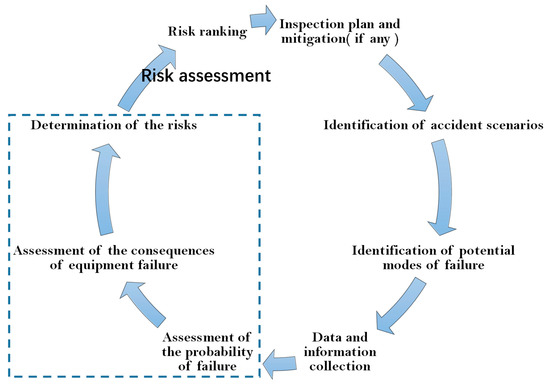
Figure 1.
The process of the generic risk-based inspection (RBI) methodology.
All these methods aim to target initial inspection resources, where the parts of the network are likely to provide the most valuable information and/or mitigate the greatest risks. At the same time, these methods are desirable for overcoming the problem of the under-inspection of higher-risk equipment and the over-inspection of lower-risk equipment [30]. Unfortunately, identifying the highest inspection priority is a non-trivial task when these methods are applied. For frequentist probability based methods, the requirement of large data is difficult to fulfill, although the well-known principles of statistical inference provide a strong basis for probability assignment in the decision making context [31]. For Bayesian probability based methods, limitations can be observed for several widely used methods, particularly for methods founded on the analytic hierarchy process (AHP) [14,24,25,29,32]. These methods suffer from limitations like the rank reversal phenomenon, shortcomings of the 1–9 ratio scale, and pitfalls in quantification of qualitatively stated pairwise comparisons [33]. Even worse, many stakeholders are often not satisfied with the results of those methods, and decision makers do not gain any confidence from such analyses. In the related analytical processes, the assessment of uncertainty is based on the subjective judgments of assessors, which problematizes the basis for the probability assignment [34].
It is worth noting that some discoveries can be made by analyzing these difficulties. First, failures of a stretch or section of a pipeline network are infrequent. The amount of failure data is too small to use frequentist probability based methods when building a model for a stretch or section of a pipeline network. However, the quantity of failure data is sufficient to build a model for the whole network via the application of other methods when aggregating all the infrequent failures that occurred in different stretches and sections of pipeline. Second, the basis for the probability assignment is noteworthy because the assumptions and hypotheses of the aforementioned approaches cannot be falsified. This is illustrated by the example of Bayesian probability based methods, which use the relative level of risk uncertainty to sort. The relative level of risk uncertainty is essentially the probability that risk event A is conditional on some background knowledge, K. Background knowledge K refers to the assumptions and hypotheses of those approaches. In theory, the conditional probability is the probability that event A is normalized to a sample space restricted to knowledge K. Due to the different knowledge K that people have, the restrictions of the sample space are different, which results in various estimations of risk uncertainty. Therefore, these estimations are more like a subjectively analyzed result without a scientific test to screen out most of them.
Based on the analysis above, we propose a spatial statistic based risk assessment approach to prioritize the inspection of pipeline networks. The advantages of this approach include the following:
- Through the application of the spatial statistic model: Poisson point process, the modeled object is transformed from a stretch or a section of a pipeline to the whole district where the pipeline network is located, which overcomes the difficulty of having insufficient data for model building.
- This approach provides a credible basis for risk assessment because the assumptions and hypotheses in our approach can be falsified by the application of statistical tests.
In the modeling process, kernel density estimation is applied to estimate the parameter of the Poisson point process. Based on that, the probability of the failure occurrence of the pipeline network in the different inspected regions is estimated. The severity of risk is measured by the total cost caused by the failures in each spatial region of the pipeline network. Then, the risks of different regions of the pipeline network can be calculated; these risks will be able to guide risk-based inspection. Finally, the application of our approach is described in a case study, and the availability is verified.
2. Poisson Point Process
The body of contemporary data on where individual pipeline failure event occurs is growing. This dataset, due to the observed spatial location of events, is called a spatial point pattern (as shown in Figure 2). The Poisson point process is fundamental to any successful analysis of spatial point patterns [35].
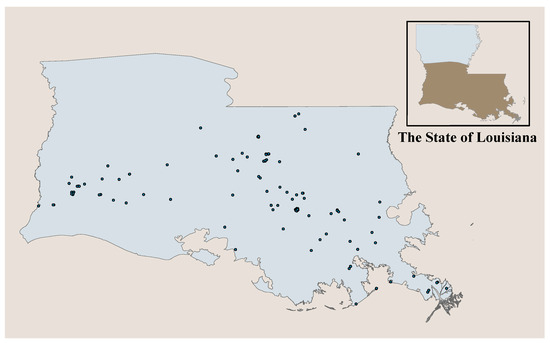
Figure 2.
The spatial point pattern of the failure events of the pipeline network in the southern part of the state of Louisiana.
Spatial point process is a random mechanism, whose outcome is a spatial point pattern . The spatial point pattern is a set of points , and it is generally represented by . The spatial point process is often defined on an observation window , inside which the point pattern is observed. In our research, the district in which the whole inspected pipeline network is located serves as the observation window (for example, the grey zone in Figure 2). For any region, the number of failure events that occur in any region is a well-defined random variable, which is denoted by . Based on that, a spatial point process on can be defined as a Poisson point process if the following two remain valid [35]:
- Poisson distribution of point counts: For any region , the number follows a Poisson distribution with the mean , which can be represented by Equation (1).
- Independent scattering: If regions ,,…, are disjointed, the counts ,…, are independent random variables.
The quantity is the expected number of failure events to occur in region , which can be calculated by Equation (2) with intensity . This intensity is interpreted as the average number of failure events occurring per unit area. If the intensity is spatially varied, the Poisson point process is called an inhomogeneous Poisson point process, which is different from a homogeneous Poisson point process, whose intensity is constant.
where is a two dimensional located point in . is the area of regions .
3. Method
The proposed approach includes three procedures: hypothesis testing, the model selection, and risk evaluation, which are shown in Figure 3. First, the reported locations of failure events in the observed window are processed using the GIS software. The aim of hypothesis testing was to validate the availability of the proposed approach. In this procedure, a hypothesis was proposed, which stated that the Poisson point process was a suitable model for the dataset of pipeline failure events. This hypothesis was tested based on the processed data. In the procedure of model selection, our approach was to determine the inhomogeneous Poisson point process or the homogeneous process to be used as the model for modeling the dataset. After that, the risks of the different inspected regions were assessed. The intensity of the chosen model was first estimated, which is the foundation for estimating the uncertainty of risk in different inspected regions. Then the consequence of risk in different inspected regions was calculated.
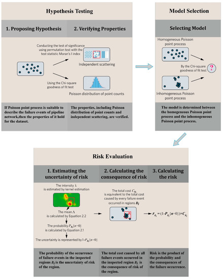
Figure 3.
The illustration of the proposed approach.
3.1. Hypothesis Testing
Based on the information in prior research [30], Poisson point process can be used to describe the failure events of a pipeline network. Therefore, the null hypothesis in our approach was stated: if the Poisson point process is suitable to describe the failure events of the pipeline network, then its properties should not be violated in the application of the proposed approach. Therefore, two properties were tested in our approach.
The first test was to verify the property of the Poisson distribution of point counts through the application of a chi-square goodness of fit test. In our approach, this hypothesis was suggested to determine whether the number of failure events that occurred in the observed window follows a Poisson distribution. The key reason for this suggestion is that any part of the observed window may not have sufficient failure event samples for the application of most statistical tests. Therefore, the observation of failure events in the observation window is chosen to test the property of the Poisson distribution of point counts with the consideration of the feasibility of tests.
Before the conduction of the first test, period must be determined, and should be considered with the inspected interval time. After that, the frequency of failure occurrence (henceforth referred to as the sample data) in the given period is obtained based on the records of the failure events. This process is illustrated in Figure 4. Then, the chi-square goodness of fit test can be implemented.
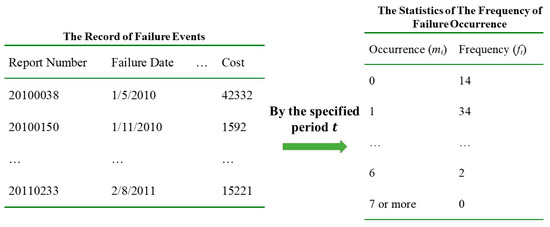
Figure 4.
The process of acquiring the sample data.
In the chi-square goodness of fit test, the null and alternative hypotheses are as follows:
H0. The quantity of pipeline failure events in region and a given period follows a Poisson distribution.
H1. The quantity of pipeline failure events in region and a given period does not follow a Poisson distribution.
Under the null hypothesis, the mean was estimated from the sample data by referring to Equation (3). Next, the theoretical frequency for each type of occurrence () was obtained by multiplying the estimated Poisson probability with the size of the sample data . The estimated Poisson probability was determined according to the Poisson distribution with the estimated . Finally, the test statistic was calculated via Equation (4) to determine whether to reject H0.
In testing the second hypothesis, the property of independent scattering was verified. The test is essentially a test of significance, which combines a permutation test with the test statistic Moran’s I index [36,37]. Moran’s I index is a commonly used spatial statistic [38], which describes autocorrelation in the spatial dimension by measuring the degree to which the number of failure events in different spatial regions of the pipeline network is similar to each other. In our approach, two groups of numbers of failure events in different spatial regions of the pipeline network were suggested for this test respectively. The first group of numbers was ,…, , counted from the inspected regions of the pipeline network (as shown in Figure 5). The second group features the counts of all districts obtained by the division of the observed window (shown in Figure 6). Both of these tests could determine whether the property of independent scattering was retained. If the property were held, we could conclude that the numbers of failure events in different spatial regions are independent Poisson random variables with the conclusions from testing the first hypothesis.
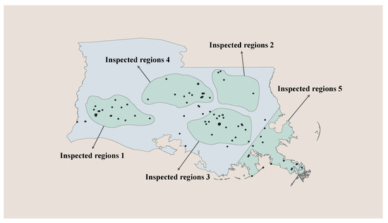
Figure 5.
The illustration of the inspected regions.
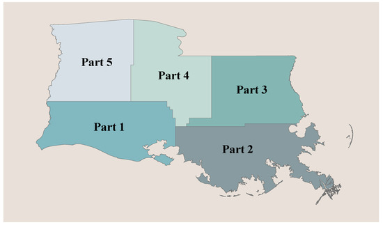
Figure 6.
The division of the observed window.
In the first step of testing the second hypothesis, the initial Moran’s I was obtained by Equation (5) based on the counts of every group. In the equation, is the element of the spatial weight matrix whose dimensions are ( is the amount of regions). The spatial weight matrix reflects the level of spatial proximity of two different regions by defining the element . In our approach, the element is obtained based on quantity and the threshold distance. If quantity is larger than the threshold distance, the element is set to 0. If not, element is equal to quantity . Quantity is calculated by the centroid distance between regions i and j. Generally, the values of Moran’s I range from −1 to +1. Values larger than indicate positive spatial autocorrelation, and a Moran’s I of less than indicates negative spatial autocorrelation.
In the second step, a permutation test was conducted. It is reasonable to believe that the counts (such as ,…, ) were randomly assigned to different regions based on the null hypothesis: the counts in different regions are spatially independent (the alternative hypothesis is that the counts in different regions are spatially dependent). Therefore, we rearranged the counts for all the different regions (such as ,…, ) and recalculated the Moran’s I value. Then, the distribution of the test statistic Moran’s I could be obtained. To calculate the p-value for the permutation test, the number of Moran’s I that was or more extreme than the initial Moran’s I was counted. Then, divided the number by the total number of Moran’s I that had been calculated. The quotient of the division was the p-value. Finally, we decided to accept the null or alternative hypothesis according to the level of significance for the test.
3.2. Model Selection
After the hypothesis testing, we could conclude that the Poisson point process was able to describe the failure events of the pipeline network. Therefore, the objective of model selection was to determine which type of Poisson point process was a suitable one. In our approach, to achieve the objective, we proposed a test that reviewed whether the intensity of the failure event is spatially variable.
In this test, the null hypothesis is stated as follows: If the homogeneous Poisson point process is a suitable model, then the intensity is not spatially variable. However, the alternative hypothesis provides no further information for the selection of models because inhomogeneous intensity or the violation of the properties of the Poisson point process can both cause a departure from the null hypothesis. Fortunately, we could eliminate the cause behind the violation of these properties according to the test results obtained during hypothesis testing. Therefore, the alternative hypothesis could be described as follows: if the inhomogeneous Poisson point process is a suitable model, then the intensity is spatially variable.
Before the test, the observation window is divided into different parts ,…, (as shown in Figure 6), all of which must have an equal area . Here, the counts ,…, are independent Poisson random variables distributed with the mean based on the null hypothesis and the assumptions above. Therefore, testing the goodness of fit of the counts to the Poisson distribution with the mean can help us to determine whether or not to reject the null hypotheses.
3.3. Risk Evaluation: The Estimation of the Probability of the Occurrence of Failure Events in Different Inspected Regions
After the determination of the type of the Poisson point process, the probability of the failure occurrence in different inspected regions can be estimated. Based on the conclusions above, it is determined that the counts ,…, of different inspected regions are independent Poisson random variables with mean ,…, based on the property of finite-dimension distribution [39]. According to Equation (2), the mean can be derived based on the intensity or . In our approach, the intensity is estimated nonparametrically via kernel estimation. The kernel estimator of the intensity in Equation (6) is thus applied; this estimator is called Diggle’s corrected estimator [40]. The kernel in our approach is the normal distribution probability density. Finally, the probability of the occurrence of failure events in region can be derived by .
where . is any spatial location inside the observation window . is the location of data point inside the observation window .
3.4. Risk Evaluation: The Estimation of the Failure Occurrence Consequence of the Pipeline Network in the Different Inspected Regions
In our approach, consequence refers to total negative set of human, environmental, and financial consequences. Its assessment focuses on the capacity of failure and subsequent events to cause death, injury, or damage to employees and/or the public, as well as to the environment. Moreover, it may also consider the consequences of failure on business, such as the costs of lost production, repair and the replacement of pipelines, and the damage to the company reputation. Accordingly, the total cost was used to measure the consequences in each region . The constitution of total cost is listed in Table 1.

Table 1.
The constitution of the total cost.
3.5. Risk Evaluation: The Determination of the Risks and Risk Ranking
In our approach, the product of the probability and consequences of failure occurrence were applied to estimate the risk related to each inspected region. Based on the obtained risk, all the regions could be ranked in order of risk; then, inspection priority could be given to each of them.
4. Case Study
The analyses in this paper were based on the southern part of the pipeline network in Louisiana state. It is defined as the observation window , whose area was approximately 98,883.802 km2. A total of 138 failure events across the observation window from January 2010 to January 2017 were analyzed. Their spatial distributions are shown in Figure 2. The data for failure events were provided by The Pipeline and Hazardous Materials Safety Administration (PHMSA). These data include the observed location of each failure event, the date that the failure event occurred, and the total cost of each failure event. In this case study, five inspected regions were established, and these regions were identified in Figure 5. Our approach was applied to evaluate the risk of each inspected region and then to identify the most critical one.
4.1. Hypothesis Testing
The property of the Poisson distribution of point counts was verified first with the application of a chi-square goodness of fit test. Before the hypothesis test, the actual number of failure events was counted under the given period (one month), which is shown in Table 2. According to the chi square distribution table, the critical value of was 12.592. Based on that value, the decision rule is defined as:
Table 2.
The monthly frequency of failure occurrence.
Reject H0 if ; otherwise, do not reject H0,
After performing the test, the decision was not to reject H0 since . There was insufficient evidence to conclude that the number of failure events that occurred monthly in the southern part of Louisiana state did not fit a Poisson distribution.
After the verification above, the property independent scattering was verified. Two groups of counts, originating from the inspected regions of the pipeline network and all districts obtained by the division of the observed window, are listed in Table 3. The spatial weight matrix of the inspected regions was created based on the threshold distance 144,420.2535 m, which is shown in Figure 7. The spatial weight matrix of all districts was created with a threshold distance 137,697.5568 m, which is shown in Figure 8. These test results are summarized in Table 4. All the results clearly indicate that we could not reject the null hypothesis. Therefore, we accepted that the property of independent scattering was retained in the two groups of counts.
Table 3.
The number of failure events in the area.
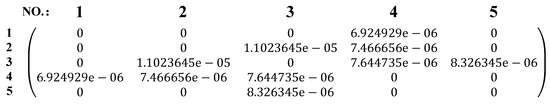
Figure 7.
The spatial weight matrix of inspected regions.
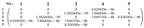
Figure 8.
The spatial weight matrix of all districts.
Table 4.
The result of the permutation test with the test statistic Moran’s I index.
4.2. Model Selection
Based on the results of the hypothesis testing, it is reasonable to believe that the Poisson point process is suitable to describe the failure events of the pipeline network in the southern part of Louisiana state. Consequently, a test reviewing whether the intensity of the failure events is spatially variable was conducted.
According to the requirements of the tests, the observation window is divided into five districts, each with an approximately equal area. By applying the null hypothesis, the expected count of each part was calculated and listed in Table 5. Then, a chi-square test was conducted. The critical value of was 9.49. Since , we rejected the null hypothesis. There was sufficient evidence to conclude that the intensity was inhomogeneous. Therefore, the application of the inhomogeneous Poisson point process was reasonable for the present dataset.
Table 5.
The areas of different districts.
4.3. The Estimation of the Probability of the Failure Occurrence of the Pipeline Network in Different Inspected Regions
After model selection, the inhomogeneous Poisson point process was determined to be the model for the spatial point pattern of pipeline failure events. Then, the intensity of the observed window was estimated through kernel estimation with a bandwidth of 11.59267 km, and the result is illustrated in Figure 9. In Figure 9, different colors are measures of intensity in different spatial location, which reflect the number of failure events occurred per square meter. Based on this intensity, the probabilities of the failure events in each inspected region were estimated.
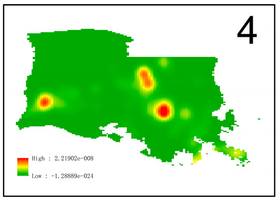
Figure 9.
The intensity of the observed window.
4.4. The Estimation of the Consequences of Failure Events of the Pipeline Network in Different Inspected Regions
To calculate the total cost of each inspected region, the total cost of each failure event in the same inspected region was added up to the total cost of the inspected region according to the items of the total cost listed in Table 1.
4.5. Determination of the Risk in Each Region and Risk Ranking
Given all the information above, the risk in each inspected region was evaluated by the production of the probability of failure, , d the measure of the consequence, .
5. Results and Discussion
After the implementation of all the steps above, the total cost and the probability of failure occurrence were calculated for each inspected region, and their risks were obtained. All these risks are listed in Table 6.
Table 6.
The result.
According to the results in Table 6, the coefficient of the variation of probability was 0.004495, which was significantly less than the coefficient of variation for the total cost, 0.878862. The small value of the coefficients of variation means that a small amount of variability existed in the data. By comparison, risk uncertainty had too small a variability in the spatial dimension, which seriously reduced the distinguishable effect of risk uncertainty. Therefore, the distinguishable effect of risk on different regions mainly originated from the consequence of risk.
Observing the mean and consequence of failure suggests a correlation between the severity of the consequence of failure and the location of its occurrence. As mentioned above, this consequence is not only determined by the location of the inspected regions but also by the frequency of the failure event in a given period. The location of the inspected region determines the total cost of each failure event in the region, and the frequency determines the number of failure events in the region. By doing a Pearson test between the mean (the mean was used to represent the frequency) and the total cost in Table 6, we found that there was no correlation between the frequency and the consequence considering that the Pearson test was −0.1128835 and the p-value for the test was 0.8566. This means that the total cost was preferably determined by location.
Considering the above observations, a qualitative comparison between our approach and existing approaches were made based on six comparison criteria. The existing approaches are categorized into other frequentist probability based methods and Bayesian probability based methods, which are limited to the items referred to in this paper. These criteria are explained in Table 7. According to the first criterion, our approach requires a medium amount of data. The amount of data required by other frequentist probability based methods may be large. For Bayesian probability based methods, empirical knowledge is a complement of other data, which effectively reduce the difficulty of acquiring input data. For the criterion of input data accessibility, our approach makes it easy to access the required data, while the existing approaches required many types of data, such as policy decision variables, failure variables, and detailed information about component characteristics and system composition, which are usually related to privacy and security issues. Therefore, these types of data are difficult to obtain. The modeling capability of our model, however, was not very good. Due to the transformation of the modeled object from a stretch or a section of a pipeline to the whole district where the pipeline network located, the spatial coordinates became a surrogate for other variables that report failure modes and system characteristics. This makes many characteristics at the component level or system level unable to be modeled, such as interdependence, a common cause of failure, which yields a decline in modeling capability. According to the criterion of computation cost, our approach had small computational cost in contrast to some approaches that use machine learning [41]. For the criterion of maturity, our approach was less mature than Bayesian probability based methods, which have been widely applied in practice with many publications. For the criterion of falsification, our approach was outstanding due to its application of hypothesis testing during modeling. In contrast, Bayesian probability based methods largely depend on empirical information and expert judgments, which are difficult to make judgments for the rationality of an analytical result.
Table 7.
Explanations of the comparison criteria.
6. Conclusions
In this study, we proposed a spatial statistic based risk assessment approach for large pipeline networks and described its application to the southern part of the pipeline network of the Louisiana state. Risk assessment is very useful for identifying the most critically inspected region. Its contributions are summarized based on its methodology, application, and theory.
For the methodology, the first contribution was exploring the application of spatial statistics in risk assessment for prioritizing pipeline inspections. As one of the most important spatial statistics technologies, the Poisson point process was used to estimate the probability of failure events occurrences in different regions of the pipeline network. The estimated probability is a more objective aleatory or stochastic than the probability estimated by Bayesian probability based methods. This means that our assessment is not vulnerable to human biases and errors. Next in importance, we tested the hypothesis of our approach to determine whether the applied assumptions and hypotheses were right or wrong. The application of a hypothesis test increased the falsifiability of risk assessment. Finally, the modeled object was transformed from a stretch or a section of pipeline to the whole district where the pipeline network was located. Being the important part of the contribution in application, it overcame the difficulty of the insufficient available data in the model building.
In application, the first contribution of this method was the application of spatial information in the records of failure events. Based on this, our approach deeply excavated the information contained in the records of failure events. The second contribution was that our approach did not require a large amount of data. Due to the transformation of the modeled object from a stretch or section of a pipeline to the whole district where the pipeline network was located, it collected all the infrequent failures records that occurred in different components of the pipeline network. In this way, the quantity of failure data was sufficient to apply our approach.
In theory, we found that risk uncertainty had too small a variability in the spatial dimension, which significantly reduced the distinguishable effect of risk uncertainty. The distinguishable effect of risk mainly originated from the consequence of risk. Therefore, uncertainty was less instructive for prioritizing pipeline inspection regions than the consequences of risk. At the same time, we found that the consequences caused by failures were more preferred to be determined by the location than risk uncertainty.
Meanwhile, the limitations of our approach could be observed from two perspectives: modeling capabilities and strict constraints. First of all, the ability of our approach to model the characteristics of a pipeline network was limited. Due to the transformation of the modeled object from a stretch or a section of the pipeline to the whole district where the pipeline network located, the spatial coordinates were a surrogate for other variables that report failure modes and system characteristics. This means that many characteristics at the components level or system level could not be modeled, such as the interdependence and common causes of failures. Therefore, the proposed method could only be used to identify high risk regions. It could not be introduced into a vulnerability analysis.
Next of importance, validating the properties of the Poisson point process is a strict constraint in the application of our approach. This constraint is a double-edged sword. Although validations increase the falsifiability of risk assessment and reduce its vulnerability to human biases and errors, the availability of our approach was significantly decreased by this validation if these properties were violated.
For future work, it will be necessary to research the factors and mechanisms that impact the severity of the consequences of failure events, in particular on the factors and the mechanisms that can be surrogated by spatial variables (such as population distribution or ecological resources). These factors can provide useful knowledge for Bayesian probability based methods in risk evaluation.
Author Contributions
Conceptualization, X.Y. and P.H.; Methodology, X.Y. and P.H.; Software, X.Y. and P.H.; Validation, X.Y., H.D. and P.H.; Formal Analysis, X.Y. and P.H.; Investigation, X.Y. and P.H.; Resources, X.Y. and P.H.; Data Curation, X.Y. and P.H.; Writing-Original Draft Preparation, X.Y. and P.H.; Writing-Review & Editing, X.Y., H.D. and P.H.; Visualization, X.Y. and P.H.; Supervision, X.Y.; Project Administration, X.Y.; Funding Acquisition, X.Y. All authors have read and agreed to the published version of the manuscript.
Funding
This research was funded by National Natural Science Foundation (No. 71801196) and National Science and Technology Major Project (2017ZX06002006).
Acknowledgments
This work was supported by National Natural Science Foundation (No. 71801196).
Conflicts of Interest
The authors declare no conflict of interest
References
- Dall’Acqua, D.; Terenzi, A.; Leporini, M.; D’Alessandro, V.; Giacchetta, G.; Marchetti, B. A new tool for modelling the decompression behaviour of CO2 with impurities using the Peng-Robinson equation of state. Appl. Energy 2017, 206, 1432–1445. [Google Scholar] [CrossRef]
- Papadakis, G.A.; Porter, S.; Wettig, J. EU Initiative on the Control of Major Accidents Hazards Arising from Pipelines. J. Loss Prev. Process Ind. 1999, 12, 85–90. [Google Scholar] [CrossRef]
- Jo, Y.D.; Ahn, B.J. A method of quantitative risk assessment for transmission pipeline carrying natural gas. J. Hazard. Mater. 2005, 123, 1–12. [Google Scholar] [CrossRef] [PubMed]
- Jamshidi, A.; Yazdani-Chamzini, A.; Yakhchali, S.H.; Khaleghi, S. Developing a new fuzzy inference system for pipeline risk assessment. J. Loss Prev. Process Ind. 2013, 26, 197–208. [Google Scholar] [CrossRef]
- American Petroleum Institute. Risk-Based Inspection: API Recommended Practice 580, 3rd ed.; American Petroleum Institute: Washington, DC, USA, 2002; ISBN 0-7176-2090-5. [Google Scholar]
- Vinod, G.; Kushwaha, H.S.; Verma, A.K.; Srividya, A. Optimisation of isi interval using genetic algorithms for risk informed in-service inspection. Reliab. Eng. Syst. Saf. 2004, 86, 307–316. [Google Scholar] [CrossRef]
- Vinod, G.; Sharma, P.K.; Santosh, T.V.; Prasad, M.H.; Vaze, K.K. New approach for risk based inspection of H2S based process plants. Ann. Nucl. Energy 2014, 66, 13–19. [Google Scholar] [CrossRef]
- Arunraj, S.; Maiti, J. Risk-based maintenance—Techniques and applications. J. Hazard. Mater. 2007, 142, 653–661. [Google Scholar] [CrossRef]
- Vind, G.; Bidhar, S.K.; Kushwaha, H.S.; Verma, A.K.; Srividya, A. A comprehensive framework for evaluation of piping reliability due to erosion-corrosion for risk-informed in-service inspection. Reliab. Eng. Syst. Saf. 2003, 84, 87–93. [Google Scholar] [CrossRef]
- Fleming, K.N. Markov models for evaluating risk-informed in-service inspection strategies for nuclear power plant piping systems. Reliab. Eng. Syst. Saf. 2004, 86, 27–45. [Google Scholar] [CrossRef]
- Vesely, W.E.; Belhadj, M.; Rezos, J.T. PRA importance measures for maintenance prioritization applications. Reliab. Eng. Syst. Saf. 1994, 43, 307–318. [Google Scholar] [CrossRef]
- Marlow, D.R.; Beale, D.J.; Mashford, J.S. Risk-based prioritization and its application to inspection of valves in the water sector. Reliab. Eng. Syst. Saf. 2012, 100, 67–74. [Google Scholar] [CrossRef]
- Luque, J.; Straub, D. Risk-based optimal inspection strategies for structural systems using dynamic Bayesian network. Struct. Saf. 2019, 76, 68–80. [Google Scholar] [CrossRef]
- Brito, A.J.; de Almeida, A.T. Multi-attribute risk assessment for risk ranking of natural gas pipelines. Reliab. Eng. Syst. Saf. 2009, 94, 187–198. [Google Scholar] [CrossRef]
- Stewart, M.G. Reliability-based assessment of ageing bridges using risk ranking and life cycle cost decision analyses. Reliab. Eng. Syst. Saf. 2001, 74, 263–273. [Google Scholar] [CrossRef]
- Aven, T.; Renn, O.; Rosa, E.A. On the ontological status of the concept of risk. Saf. Sci. 2011, 49, 1074–1079. [Google Scholar] [CrossRef]
- Aven, T. The risk concept—Historical and recent development trends. Reliab. Eng. Syst. Saf. 2012, 99, 33–44. [Google Scholar] [CrossRef]
- Aven, T.; Renn, O. On risk defined as an event where the outcome is uncertain. J. Risk Res. 2009, 12, 1–11. [Google Scholar] [CrossRef]
- Najafi, M.; Kulandaivel, G. Pipeline condition prediction using neural network models. In Proceedings of the Pipeline Division Specialty Conference 2005, Houston, TX, USA, 21–24 August 2005; pp. 767–781. [Google Scholar] [CrossRef]
- Baik, H.S.; Jeong, H.S.; Abraham, D.M. Estimating transition probabilities in Markov chain-based deterioration models for management of wastewater systems. J. Water Resour. Plan. Manag. 2006, 132, 15–24. [Google Scholar] [CrossRef]
- Khan, Z.; Zayed, T.; Moselhi, O. Simulating impact of factors affecting sewer network operational condition. In Proceedings of the CSCE 2009 Annual General Conference, St. John’s, NL, Canada, 27–30 May 2009; pp. 285–294. [Google Scholar]
- Fuchs-Hanusch, D.; Friedl, F.; Mo€derl, M.; Sprung, W.; Plihal, H.; Kretschmer, F.; Ertl, T. Risk and performance oriented sewer inspection prioritization. In Proceedings of the World Environmental and Water Resources Congress 2012: Crossing Boundaries, Albuquerque, NM, USA, 20–24 May 2012; pp. 3711–3723. [Google Scholar]
- Hahn, M.A.; Palmer, R.N.; Merrill, S.M. Prioritizing sewer line inspection with an expert system. In Proceedings of the 26th Annual Water Resources Planning and Management Conference, Tempe, AZ, USA, 6–9 June 1999; pp. 1–9. [Google Scholar]
- Hahn, M.A.; Palmer, R.N.; Merrill, S.M.; Lukas, A.B. Expert system for prioritizing the inspection of sewers: Knowledge base formulation and evaluation. J. Water Resour. Plan. Manag. 2002, 128, 121–129. [Google Scholar] [CrossRef]
- Dey, P.K. Analytic hierarchy process analyzes risk of operating cross-country petroleum pipelines in India. Nat. Hazards Rev. 2003, 4, 213–221. [Google Scholar] [CrossRef]
- Dey, P.K.; Ogunlana, S.O.; Naksuksakul, S. Risk-based maintenance model for offshore oil and gas pipelines: A case study. J. Qual. Maint. Eng. 2004, 10, 169–183. [Google Scholar] [CrossRef]
- Anbari, M.J.; Tabesh, M.; Roozbahani, A. Risk assessment model to prioritize sewer pipes inspection in wastewater collection networks. J. Environ. Manag. 2017, 190, 91–101. [Google Scholar] [CrossRef] [PubMed]
- Kaplan, S.; Garrick, B.J. On The Quantitative Definition of Risk. Risk Anal. 1981, 1, 11–27. [Google Scholar] [CrossRef]
- Mancuso, A.; Compare, M.; Salo, A.; Zio, E.; Laakso, T. Risk-based optimization of pipe inspections in large underground networks with imprecise information. Reliab. Eng. Syst. Saf. 2016, 152, 228–238. [Google Scholar] [CrossRef]
- Cagno, E.; Caron, F.; Mancini, M.; Ruggeri, F. Using AHP in determining the prior distributions on gas pipeline failures in a robust Bayesian approach. Reliab. Eng. Syst. Saf. 2019, 67, 275–284. [Google Scholar] [CrossRef]
- Geary, W. Risk Based Inspection: A Case Study Evaluation of Offshore Process Plant; Health and Safety Laboratory: Sheffield, UK, 2002. [Google Scholar]
- Aven, T.; Zio, E. Some consideration on the treatment of uncertainties in risk assessment for practical decision making. Reliab. Eng. Syst. Saf. 2011, 96, 64–74. [Google Scholar] [CrossRef]
- Zio, E. The Future of Risk Assessment. Reliab. Eng. Syst. Saf. 2018, 177, 176–190. [Google Scholar] [CrossRef]
- Aven, T. On the new ISO guide on risk management terminology. Reliab. Eng. Syst. Saf. 2017, 96, 719–726. [Google Scholar] [CrossRef]
- Dietrich, S.; Penttinen, A. Recent Applications of Point Process Methods in Forestry Statistics. Stat. Sci. 2000, 15, 61–78. [Google Scholar] [CrossRef]
- Sloane, D.; Morgan, S.P. An Introduction to Categorical Data Analysis. Annu. Rev. Sociol. 1996, 22, 351–375. [Google Scholar] [CrossRef]
- Niknian, M. Permutation Tests: A Practical Guide to Resampling Methods for Testing Hypotheses. Technometrics 1994, 37, 341–342. [Google Scholar] [CrossRef]
- Hongfei, L.; Calder, C.A.; Cressie, N. Beyond Moran’s I: Testing for Spatial Dependence Based on the Spatial Autoregressive Model. Geogr. Anal. 2007, 39, 357–375. [Google Scholar] [CrossRef]
- Daley, D.J.; Vere-Jones, D. An Introduction to the Theory of Point Processes, Vol.II: Probability and Its Applications; Springer: NY, USA, 2008; ISBN 978-0-387-21337-8. [Google Scholar]
- Diggle, P. A Kernel Method for Smoothing Point Process Data. J. R. Stat. Soc. Ser. C Appl. Stat. 1985, 34, 138–147. [Google Scholar] [CrossRef]
- Rachman, A.; Ratnayake, R.C. Machine learning approach for risk-based inspection screening assessment. Reliab. Eng. Syst. Saf. 2019, 185, 518–532. [Google Scholar] [CrossRef]


© 2020 by the authors. Licensee MDPI, Basel, Switzerland. This article is an open access article distributed under the terms and conditions of the Creative Commons Attribution (CC BY) license (http://creativecommons.org/licenses/by/4.0/).