Hydrate Production Philosophy and Thermodynamic Calculations

Abstract

The amount of energy in the form of natural gas hydrates is huge and likely substantially more than twice the amount of worldwide conventional fossil fuel. Various ways to produce these hydrates have been proposed over the latest five decades. Most of these hydrate production methods have been based on evaluation of hydrate stability limits rather than thermodynamic consideration and calculations. Typical examples are pressure reduction and thermal stimulation. In this work we discuss some of these proposed methods and use residual thermodynamics for all phases, including the hydrate phase, to evaluate free energy changes related to the changes in independent thermodynamic variables. Pressures, temperatures and composition of all relevant phases which participate in hydrate phase transitions are independent thermodynamic variables. Chemical potential and free energies are thermodynamic responses that determine whether the desired phase transitions are feasible or not. The associated heat needed is related to the first law of thermodynamics and enthalpies. It is argued that the pressure reduction method may not be feasible since the possible thermal gradients from the surroundings are basically low temperature heat that is unable to break water hydrogen bonds in the hydrate–water interface efficiently. Injecting carbon dioxide, on the other hand, leads to formation of new hydrate which generates excess heat compared to the enthalpy needed to dissociate the in situ CH₄ hydrate. But the rapid formation of new CO₂ hydrate that can block the pores, and also the low permeability of pure CO₂ in aquifers, are motivations for adding N₂. Optimum mole fractions of N₂ based on thermodynamic considerations are discussed. On average, less than 30 mole% N₂ can be efficient and feasible. Thermal stimulation using steam or hot water is not economically feasible. Adding massive amounts of methanol or other thermodynamic inhibitors is also technically efficient but far from economically feasible.

1. Introduction

The huge amounts of worldwide energy resources in the form of hydrate are huge. Estimates vary but in view of estimates from USGS from 2000 and the rapid discovery of new hydrate resources it is likely substantially more than twice all known resources of conventional fossil fuels. Most of these hydrates are generated from biogenic hydrocarbon sources, and almost pure methane hydrate. These hydrates are structure I hydrates. Thermogenic sources of hydrocarbons will make a mixture of structure I and II which depends on the hydrocarbon composition. As long as there is availability of propane and iso-butane, structure II formation will dominate. Structure II hydrate contains 16 small cavities and 8 large cavities with a total of 136 water molecules in a unit cell with side lengths of 17 Å. The small cavity is similar to the small cavity in structure I but the large cavity in structure II is larger and contains 28 water molecules in the cavity walls. The combination of a good stabilization by propane and iso-butane of the large cavity, and stabilization of the small cavity by methane, result in low free energy hydrate. Dynamically propane, iso-butane, CO₂ and H₂S are superior in adsorption on liquid water [1] as compared to supercritical CH₄. Even from a thermodynamic point of view it is the properties (chemical potentials and densities) of molecules in the water/gas interface region that determines the hydrate formation pattern and hydrate composition.

There are also other hydrate structures but the cavity size distribution makes them more exotic and rare in nature, although structure H has been identified in a few places in the Gulf of Mexico [2]. In view of CH₄ hydrate dominance in nature, we will limit our discussion to these hydrates in order to simplify the problem and illustrate the thermodynamic analysis.

The paper is organized as follows. The next section gives a fairly basic introduction to multiphase thermodynamics in order to clarify a number of misunderstandings related to hydrates in sediments, and frequent assumptions (and use) of thermodynamic equilibrium. For this reason there are unfortunately few references to other theoretical papers related to CO₂ exchange of in situ CH₄ hydrate. Mechanisms involved in the conversion are also a limiting factor in some other papers on this system. In the following section we discuss the impact of mineral surfaces on fluid/hydrate thermodynamics and hydrate nucleation aspects. Pressure reduction has been a dominant technology platform for producing hydrates in experiments and pilots. Some important drawbacks and limitations of this approach are discussed in Section 5, followed by a discussion of CO₂ injection as a possible win-win approach for energy production and safe storage of CO₂. A discussion follows in Section 7 before our conclusions.

2. Theoretical Background

Despite the simplicity of only one hydrate former and water, the system is complicated by the fact that hydrates inside sediments are exposed to the issue of there being too many independent variable defined and fixed locally, compared to the number of independent variables that can be defined in order to ensure thermodynamic equilibrium. Temperature is always defined by geothermal gradients and some impact of flow through the sediments, which mix in fluids from neighboring parts (different temperatures) of sediments. Pressure is defined by hydrostatics and hydrodynamics.

The simplest system of these two components is the region of temperatures and pressures in which only two phases exist. This is thermodynamically a very trivial system but still convenient to start with in the derivation of thermodynamic non-equilibrium. If water and CH₄ is totally isolated at constant volume then the first law for the composite system of these two phases is:

$$d{\underset{-}{U}}^{(aq)}=d{Q}^{(aq)}-P^{(aq)}d{\underset{-}{V}}^{(aq)}+{\displaystyle \sum _{i=1}^n{\mu }_i^{(aq)}d{N}_i^{(aq)}}$$

(1)

$$d{\underset{-}{U}}^{(gas)}=d{Q}^{(gas)}-P^{(gas)}d{\underset{-}{V}}^{(gas)}+{\displaystyle \sum _{i=1}^n{\mu }_i^{(gas)}d{N}_i^{(gas)}}$$

(2)

The water phase is denoted as aq and the CH₄ phase is denoted as gas. U is internal energy and the line beneath denotes extensive energy with the unit Joule. The line under the volume V denotes extensive volume in m³. N is number of moles and index I is a counter on components. In this case i is either CH₄ or water. The two first terms are trivial in terms of the added heat and the delivered mechanical work, while the last term is frequently denoted as the chemical work. Basically it the work needed release (negative dN_i) molecules from the actual phase. The chemical potential ${\mu }_i^{(aq)}$ is the driving force for this release, and consists of a necessary energy to release the molecules from attractions to surrounding molecules, and an entropy contribution related to rearrangements of the remaining molecules.

Since the system is isolated then:

$$d{\underset{-}{U}}^{(aq)}+d{\underset{-}{U}}^{(gas)}=0$$

(3)

$$d{Q}^{(aq)}+d{Q}^{(gas)}=0$$

(4)

$$d{\underset{-}{V}}^{(gas)}+d{\underset{-}{V}}^{(aq)}=0$$

(5)

$$d{N}_i^{(gas)}+d{N}_i^{(aq)}=0$$

(6)

The second law of thermodynamics for the system is:

$$d\underset{-}{S}=d{\underset{-}{S}}^{(gas)}+d{\underset{-}{S}}^{(aq)}\ge 0$$

(7)

$$\frac{d{Q}^{(aq)}}{T^{(aq)}}=d{\underset{\leftharpoondown }{S}}^{(aq)}$$

(8)

$$\frac{d{Q}^{(gas)}}{T^{(gas)}}=d{\underset{\leftharpoondown }{S}}^{(gas)}$$

(9)

Combining Equations (1), (4), (7) and (8) gives:

$$d{\underset{-}{U}}^{(aq)}\le T^{(gas)}d{\underset{-}{S}}^{(aq)}-P^{(aq)}d{\underset{-}{V}}^{(aq)}+{\displaystyle \sum _{i=1}^n{\mu }_i^{(aq)}d{N}_i^{(aq)}}$$

(10)

Combining Equations (2), (4), (7) and (9) gives:

$$d{\underset{-}{U}}^{(gas)}\le T^{(aq)}d{\underset{-}{S}}^{(gas)}-P^{(gas)}d{\underset{-}{V}}^{(gas)}+{\displaystyle \sum _{i=1}^n{\mu }_i^{(gas)}d{N}_i^{(gas)}}$$

(11)

(7), (10) and (11) using (3), (5) and (6) gives:

$$\begin{array}{l}d{\underset{\leftharpoondown }{S}}^{rotal}\ge d{\underset{\leftharpoondown }{U}}^{(gas)}\left[\frac{1}{T^{(aq)}}-\frac{1}{T^{(gas)}}\right]-d{\underset{\leftharpoondown }{V}}^{(gas)}\left[\frac{P^{(gas)}}{T^{(aq)}}-\frac{P^{(aq)}}{T^{(gas)}}\right]\\ +{\displaystyle \sum _{}^{}\left[\frac{{\mu }_j^{(gas)}}{T^{(aq)}}-\frac{{\mu }_j^{(aq)}}{T^{(gas)}}\right]}d{N}_i^{(gas)}\ge 0\end{array}$$

(12)

The only absolute solutions that make stability possible for the system is when the entropy change approaches unconditionally zero when all the terms in the brackets in (12) approach zero.

$$T^{(aq)}=T^{(gas)}$$

(13)

$$P^{(aq)}=P^{(gas)}$$

(14)

$${\mu }_i^{(aq)}(T^{(aq)},T^{(aq)},{\overrightarrow{x}}^{(aq)})={\mu }_i^{(gas)}(T^{(gas)},T^{(gas)},{\overrightarrow{y}}^{(gas)})$$

(15)

Equation (13) implies that there is no net heat transport between the two phases, Equation (14) is simply Newton’s second law while (15) suggests that the average net mass transport between the two phases is zero.

In terms of (15) the number of moles in each phase is not relevant and the conservation of mass reduces to the conservation of mole-fractions in each phase.

Legendre transforms of (10) and (11) in terms of the entropy results in Helmholtz free energy ${\underset{-}{A}}^{total}$, and the final result for the total system is:

$$\begin{array}{l}d{\underset{-}{A}}^{total}\le {\underset{-}{-S}}^{(aq)}d{T}^{(gas)}-P^{(aq)}d{\underset{-}{V}}^{(aq)}+{\displaystyle \sum _{i=1}^n{\mu }_i^{(aq)}d{N}_i^{(aq)}}\\ -{\underset{-}{S}}^{(gas)}d{T}^{(aq)}-P^{(gas)}d{\underset{-}{V}}^{(gas)}+{\displaystyle \sum _{i=1}^n{\mu }_i^{(gas)}d{N}_i^{(gas)}}\end{array}$$

(16)

Equation (16) is the formal thermodynamic basis for Phase Field Theory [2,3,4,5,6,7,8,9,10,11,12] (and references in these) modelling, which will also then include the work of pushing away the original phases to create space for new phase(s).

For flowing systems it is convenient to extract the internal push work. Legendre transforms of the mechanical work terms leads to Gibb’s free energy ${\underset{-}{G}}^{total}$ for the system, in Equation (17) below.

$$\begin{array}{l}d{\underset{-}{G}}^{total}\le {\underset{-}{-S}}^{(aq)}d{T}^{(gas)}+{\underset{-}{V}}^{(aq)}d{P}^{(aq)}+{\displaystyle \sum _{i=1}^n{\mu }_i^{(aq)}d{N}_i^{(aq)}}\\ -{\underset{-}{S}}^{(gas)}d{T}^{(aq)}-{\underset{-}{V}}^{(gas)}d{P}^{(gas)}+{\displaystyle \sum _{i=1}^n{\mu }_i^{(gas)}d{N}_i^{(gas)}}\end{array}$$

(17)

The number of independent variables in Equations (13)–(15) is 8 and the number of conservation equations and conditions of equilibrium, Equations (13)–(15), is 6. Mathematically this system can be solved if two of the independent variables are defined, as also indicated in

Table 1. Numbers of independent thermodynamic variables versus conservation laws and equilibrium equations.

Var. no.	Variable	Eq, no	Equation	Diff.
1	$x_{C{H}_4}^{gas}$	1	$x_{C{H}_4}^{gas}+x_{H_{2}O}^{gas}=1$
2	$x_{C{H}_4}^{aq.}$	2	$x_{C{H}_4}^{aq.}+x_{H_{2}O}^{aq.}=1$
3	$x_{H_{2}O}^{gass}$	3	$T_{}^{gas}=T_{}^{aq}$
4	$x_{H_{2}O}^{aq.}$	4	$P_{}^{gas}=P_{}^{aq}$
5	$T_{}^{gas}$	5	${\mu }_{C{H}_4}^{gas}={\mu }_{C{H}_4}^{aq}$
6	$T_{}^{aq}$	6	${\mu }_{H_{2}O}^{gas}={\mu }_{H_{2}O}^{aq}$
7	$P_{}^{gas}$
8	$P_{}^{aq}$
2 phase	8	6		2
9	$x_{C{H}_4}^H$	7	$x_{C{H}_4}^H+x_{H_{2}O}^H=1$
10	$x_{H_{2}O}^H$	8	$T_{}^H=T_{}^{aq}$
11	$T_{}^H$	9	$P_{}^H=P_{}^{aq}$
12	$P_{}^H$	10	${\mu }_{C{H}_4}^H={\mu }_{C{H}_4}^{aq}$
		11	${\mu }_{H_{2}O}^H={\mu }_{H_{2}O}^{aq}$
3 phase	12	11		1
13	$x_{C{H}_4}^{H_{aq}}$	12	$x_{C{H}_4}^{H_{aq}}+x_{H_{2}O}^{H_{aq}}=1$
14	$x_{H_{2}O}^{H_{aq}}$	13	$T_{}^{H_{aq}}=T_{}^{aq.}$
15	$T_{}^{H_{aq}}$	14	$P_{}^{H_{aq}}=P_{}^{aq.}$
16	$P_{}^{H_{aq}}$	15	${\mu }_{C{H}_4}^{H_{aq}}={\mu }_{C{H}_4}^{aq}$
		16	${\mu }_{H_{2}O}^{H_{aq}}={\mu }_{H_{2}O}^{aq}$
4 phase	16	16		0
17	$x_{C{H}_4}^{ads.}$	17	$x_{C{H}_4}^{ads.}+x_{H_{2}O}^{ads.}=1$
18	$x_{H_{2}O}^{ads.}$	18	$T_{}^{ads.}=T_{}^{aq.}$
19	$T_{}^{ads.}$	19	$P_{}^{a.ds}=P_{}^{aq.}$
20	$P_{}^{ads.}$	20	${\mu }_{C{H}_4}^{ads.}={\mu }_{C{H}_4}^{aq}$
		21	${\mu }_{H_{2}O}^{ads}={\mu }_{H_{2}O}^{aq}$
5 phase	20	21		−1
21	$x_{C{H}_4}^{H,ads.}$	22	$x_{C{H}_4}^{H,ads.}+x_{H_{2}O}^{H,ads.}=1$
22	$x_{H_{2}O}^{H,ads.}$	23	$T_{}^{H,ads.}=T_{}^{aq.}$
23	$T_{}^{H,ads.}$	24	$P_{}^{H,ads}=P_{}^{aq.}$
24	$P_{}^{H,ads.}$	25	${\mu }_{C{H}_4}^{H,ads.}={\mu }_{C{H}_4}^{aq.}$
		26	${\mu }_{H_{2}O}^{H,ads.}={\mu }_{H_{2}O}^{aq.}$
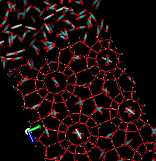
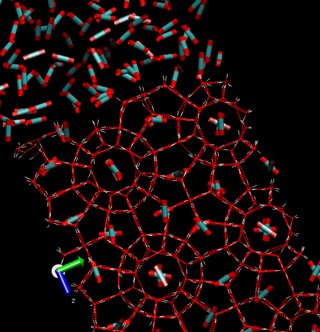
6 phase	24	26		–2

below. A schematic illustration of structure I hydrate is provided in Figure 1. This is a snapshot from a Molecular Dynamics simuation set-up in which the guest molecules are scaled down. In Table 1 we limit ourselves to counting only two hydrates. One hydrate is formed between gas hydrate former from a separate. A second hydrate phase if formed from hydrate former dissolved in liquid water.

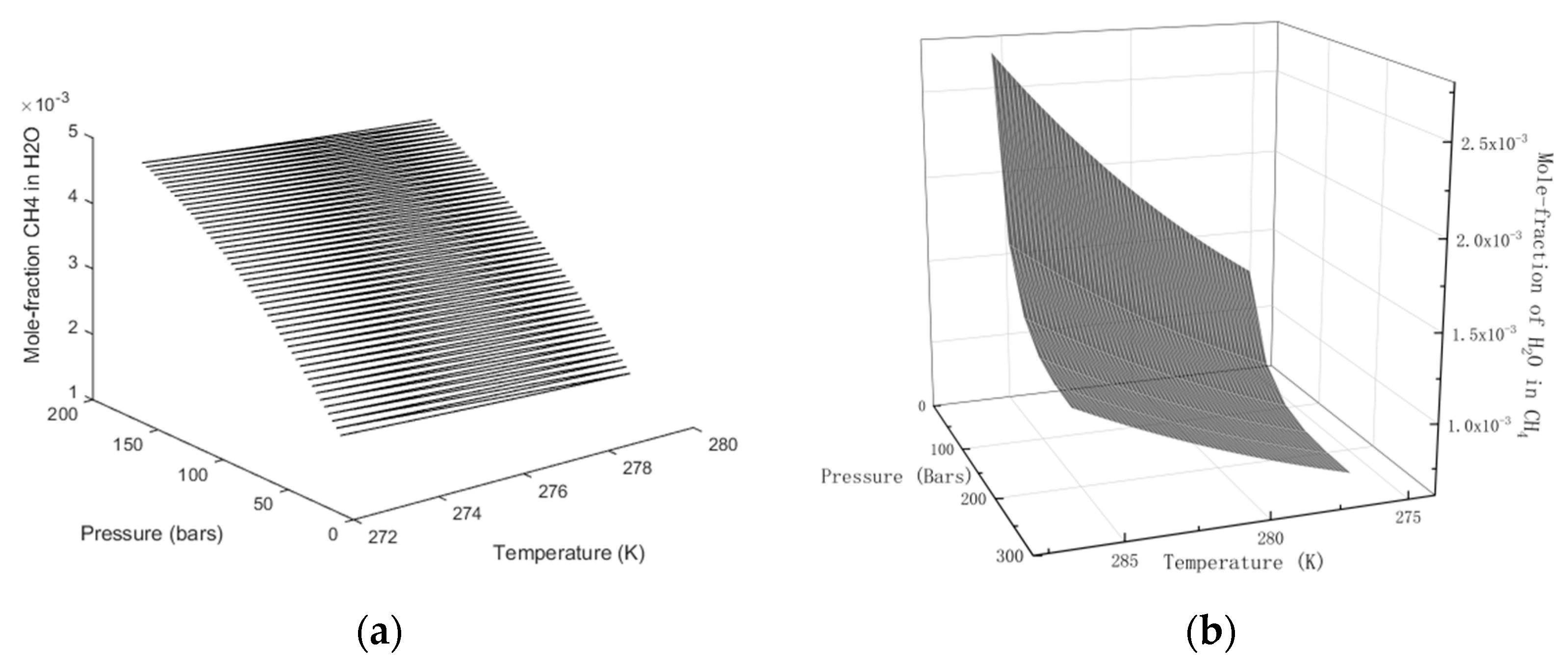
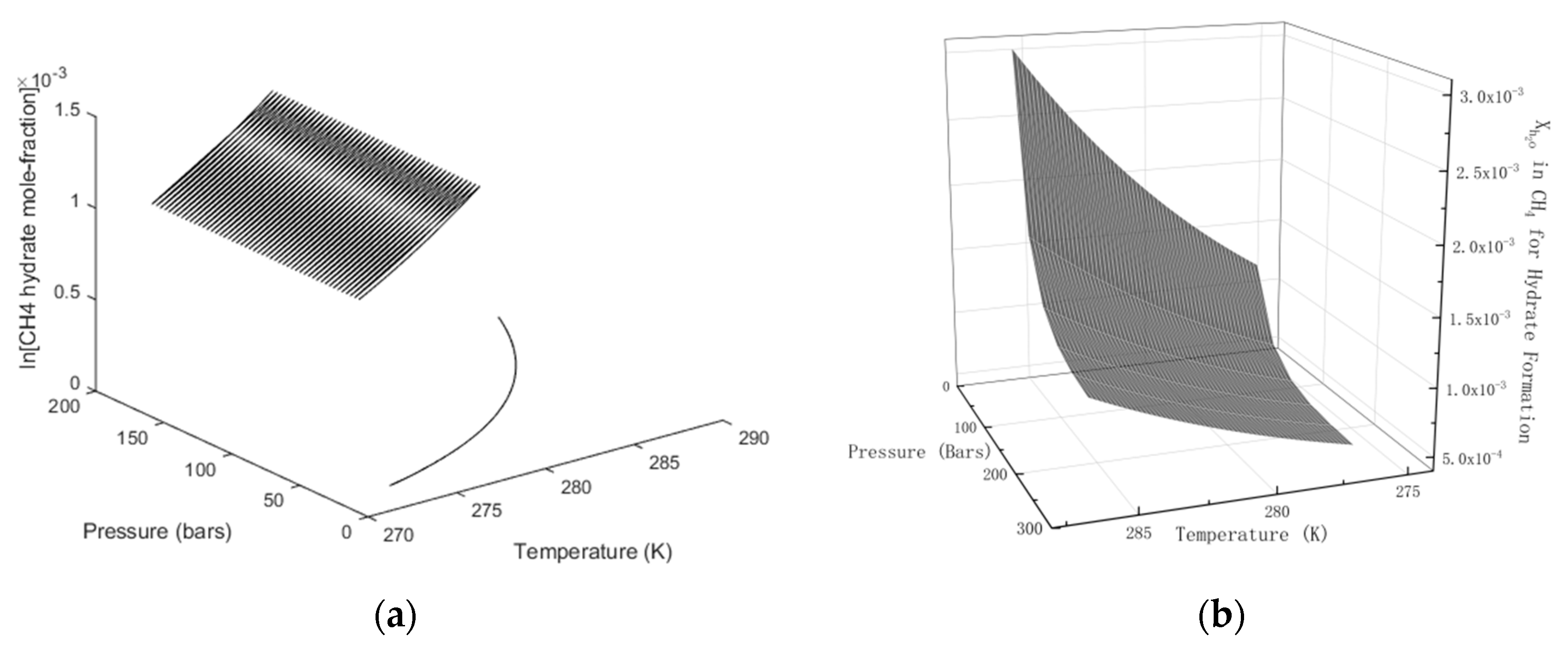
Detailed models for water and methane chemical potentials in the two phases can be found in Kvamme [13,14] and Kvamme et.al. [15] and will not be repeated here. Numerical solutions for the distribution of the two components in gas and water for various combinations of temperature and pressure are given in Figure 2.

Moving the system into the hydrate-forming region of temperature and pressure now reduces the system to 1 degree of freedom. In practical terms, this means that only one independent variable can be defined if the system should be able to reach thermodynamic equilibrium. This is well known in measurements of hydrate equilibrium. Classically it has often been measured by the hydrate dissociation temperature for a fixed pressure. But there is a theoretical ambiguity to this, which is visible when looking at models for hydrate from statistical mechanics.

Van der Waals and Platteeuw [16] used a semi Grand Canonical ensemble to derive a Langmuir-type adsorption theory in which water molecules are fixed and rigid while molecules that enter cavities (guest molecules) are open to exchange with surrounding phases. The final result of the derivation is expressed in terms of chemical potential for water in hydrate:

$${\mu }_{H_{2}O}^H={\mu }_{H_{2}O}^{O,H}-{\displaystyle \sum }_{k=1,2}RT{v}_k\ln \left(1+{\displaystyle \sum }_i{h}_{ij}\right)$$

(18)

${\mu }_{H_{2}O}^{O,H}$ is the chemical potential for water in an empty clathrate for the given structure in consideration. k is an idex for cavity types and j is an index for guest molecules in the various cavities. The number of cavities is ν, with bubscripts k for large and small cavities respectively. For structure I, which is the main focus here, ν_large = 3/24 and ν_small = 1/24. For structure II the corresponding numbers are ν_large = 1/17 and ν_small = 2/17.

Historically, thus, value has not been calculated by theoretical methods but rather fitted to experimental data in the form of chemical potential of pure liquid water minus empty clathrate water chemical potential. Kvamme and Tanaka [17] used molecular dynamics simulations to calculate empty clathrate water chemical potentials, as well as chemical potentials for ice and liquid water. In contrast to the original van der Waals and Platteuw [16] derivation, the canonocal partition function for the cavities (see below) is not contrained to a rigid water lattice in the formulation of Kvamme the Tanaka [17]. Harmonic oscillator models for large guest molecules relative to cavity is more accurate than rigid water lattice model, and samplings directly points at frequencies of guest movement that affects water librations. Smaller guest molecules are better represented by the classical integration over Boltzmann factors for interactions between water and guest in the cavity volume.

Most hydrate codes use the original van der Waals and Platteeuw [16] with a fixed lattice and fugacity instead of chemical potentials to desctibe hydrate former phase. See Sloan and Koh [18] for the historical treatment of hydrate phase transitions and equilibrium. See also Kvamme and Førrisdahl [19] for polar guest molecules and Kvamme and Lund [20] for effects of guest-guest interactions.

$$h_{ki}=e^{\beta \left[{\mu }_{ki}{}^H(T,P,{\overrightarrow{x}}^H)-\mathsf{\Delta }{g}_{ki}(T)\right]}$$

(19)

where β is the inverse of the universal gas constant times temperature. At equilibrium, the chemical potential of the guest molecules i in hydrate cavity k is equal to the chemical potential of molecules i in the co-existing phase it comes from. For non-equilibrium, the chemical potential is adjusted for distance from equilibrium through a Taylor expansion.

$$\begin{array}{l}{\mu }_{ki}^H(T,P,{\overrightarrow{x}}^H)={\mu }_{ki}^H(T^{Eq.},P^{Eq.},{\overrightarrow{x}}^{H,Eq.})\\ +{\displaystyle \sum _r}{\frac{\partial {\mu }_{ki}^H(T,P,{\overrightarrow{x}}^H)}{\partial x_r}|}_{P,T,x_{i\ne r}}\left(x_r^{}-x_r^{H,Eq.}\right)\\ +{\frac{\partial {\mu }_{ki}^H(T,P,{\overrightarrow{x}}^H)}{\partial P}|}_{T,\overrightarrow{x}}\left(P-P^{H,Eq.}\right)+{\frac{\partial {\mu }_{ki}^H(T,P,{\overrightarrow{x}}^H)}{\partial T}|}_{P,\overrightarrow{x}}(T-T^{Eq.})\end{array}$$

(20)

Examples of free energies of inclusion (latter term in the exponent) are reported elsewhere [21,22,23,24,25]. At thermodynamic equilibrium between a free hydrate former phase, ${\mu }_{ki}$ is the chemical potential of the guest molecule in the hydrate former phase (gas, liquid, or fluid) at the hydrate equilibrium temperature and pressure.

The composition of the hydrate is also trivially given by the derivation from the semi-grand canonical ensemble and given by:

$${\theta }_{ki}=\frac{h_{ki}}{1+{\displaystyle \sum _j{h}_{ki}}}$$

(21)

${\theta }_{ki}$ is the filling fraction of component i in cavity type k. Also:

$$x_{i,l\arg e}^H=\frac{{\theta }_{l\arg e,i}{\nu }_{l\arg e}}{1+{\theta }_{l\arg e,i}{\nu }_{l\arg e}+{\theta }_{small,i}{\nu }_{small}}$$

(22)

$$x_{i,small}^H=\frac{{\theta }_{small,i}{\nu }_{small}}{1+{\theta }_{l\arg e,i}{\nu }_{l\arg e}+{\theta }_{small,i}{\nu }_{small}}$$

(23)

where ν is the fraction of cavity per water for the actual cavity type, as indicated by subscripts. The corresponding mole-fraction water is then given by:

$$x_{H_{2}O}^H=1-{\displaystyle \sum _i{x}_{i,l\arg e}^H}-{\displaystyle \sum _i{x}_{i,small}^H}$$

(24)

and the associated hydrate free energy is then:

$$G^{(H)}=x_{H_{2}O}^H{\mu }_{H_{2}O}^H+{\displaystyle \sum _i{x}_i^H{\mu }_i^H}$$

(25)

The composition of the initial hydrate, and the free energy of the hydrate created initially, depends on the conditions of temperature and pressure at which the hydrate was formed. But a review of experimental data and experimental methods is outside the scope of this work.

Temperature and pressure are always both defined in real cases. For hydrates in nature the temperature is controlled by geothermal gradients and flow, and pressure is defined by hydrostatics and flow. Hydrate formation in pipelines and industrial equipment is always happening at locally defined temperatures and pressures. Heat transport is typically 2–3 orders of magnitude faster than mass transport [7] (and enclosed papers) in water systems, but slow through CH₄. Mechanical stability between liquid water and hydrate is fast but mechanical stability between gas phase and other phases is slower.

What is important, however, is that there is no simple rule on equal chemical potentials for all components in all phases. Local chemical potentials of all components in all phases, and corresponding distribution of masses over the various phases are determined by an extension of (17) to include all co-existing phases, under constraints of mass and heat transport. An important implication of this is that the chemical potential of CH₄ in the gas phase can generally be different from the chemical potential for CH₄ in the water phase. With reference to (19) and (21) to (25) we can expect at least two different hydrates, one type of hydrate formed from gas CH₄ and water and another hydrate from CH₄ dissolved in water. The degrees of freedom will, therefore, reduce to zero and the system is mathematically over-determined by two independent thermodynamic variables.

In Figure 3 we plot the limits of hydrate stability in pressure, temperature and concentration of CH₄ in surrounding water, and in Figure 3b we plot the stability limits of hydrate as a function of concentration for variations of temperature and pressure. I.e.: Even if hydrate forms according to the temperature and pressure stability limits in Figure 3a there will still be competing processes of hydrate dissociation if the surrounding water contains less CH₄ than the black contour for concentrations as functions of temperature and pressure. Hydrate can form from concentrations in between the concentration contour in Figure 2a and the lowest limit of hydrate stability in Figure 3a. Hydrate formation from gas is theoretically possible for water concentrations equal to, or higher, than the values in the contour of Figure 3b. Any water concentrations lower than concentrations in Figure 3b will lead to hydrate sublimation. While hydrate is, theoretically, possible from dissolved water in gas, from a thermodynamic point of view, it is obvious that the logistics of merging water molecules enough to create hydrate is a challenge. Getting rid of formation heat adds to the challenge. CH₄ gas is an efficient heat insulator.

As will be discussed in more detail later, the three different situations in Figure 3 give different hydrates. Hydrate formation from gas will not be discussed further since it is not important and even unlikely to happen due to limitations in mass and heat transport. But hydrates from solution can be far more than just one since the contours in Figure 3a is the lowest limit of hydrate stability and the hydrates of lowest stability. The closer the water concentration approaches the concentrations in Figure 2a, the more stable the hydrate that is formed. From a mathematical perspective the concentration ranges between the concentration contours in Figure 2a and Figure 3a an infinite number of different hydrates can be formed from solution of CH₄ in water. In practical terms, there will of course be competition on mass which over time will lead to reorganization in the direction that more stable hydrates will consume less stable hydrate.

In the more general situation the combination of first and second laws of thermodynamics can be expressed by Equation (26) for a number of different phases. m is a phase index and m, surr. denotes temperature effects from all surroundings and will not be a single source and one temperature in a general non-equilibrium situation. In contrast to energy and mass entropy-related quantities are non-conserved and (26) simply says that the system will locally develop towards minimum free energy as a function of the independent thermodynamic variables in the system. If we assume that the multi-phase version of Equations (13) and (14) are fulfilled then the minimum of Equation (26), under constraints of mass and energy conservation, gives the thermodynamically most likely distribution of phases, and associated composition of these phases.

$$d{\underset{-}{G}}^{total}\le {\displaystyle \sum _{m=1}^{phases}{\underset{-}{-S}}^{(m)}d{T}^{(m,surr.)}+{\underset{-}{V}}^{(m)}d{P}^{(m)}+{\displaystyle \sum _{i=1}^{n.m}{\mu }_i^{(m)}d{N}_i^{(m)}}}\le 0$$

(26)

The minimum of Equation (26) does not mean that each local phase at a given time is unconditionally stable. Quite the opposite is true. For a phase to be unconditionally stable the additional constraints must be fulfilled:

$${\left[\frac{\partial {\underset{\_}{G}}^{(m)}}{\partial M}\right]}_{K\ne M}\delta M\le 0$$

(27)

for any possible range of changes of independent variable M.

The symbol K is used as a general index for thermodynamic variables in all co-existing phases. M is also an index for all independent thermodynamic variables in all co-existing phases. For a flowing system the energy level is most conveniently expressed in terms of enthalpy and the enthalpy corresponding to the same multi-components system is given by:

$$d{\underset{-}{H}}^{total}\le {\displaystyle \sum _{m=1}^{phases}d{Q}^{(m)}+{\underset{-}{V}}^{(m)}d{P}^{(m)}+{\displaystyle \sum _{i=1}^{n.m}{\mu }_i^{(m)}d{N}_i^{(m)}}}$$

(28)

Superscript m indicates added heat to phase m from any surrounding, including all other phases and external sources.

Equations (26)–(28) express, in short, the motivation of this paper. Very often hydrate production potential is evaluated based on projections of independent thermodynamic variables with careful calculations of whether the thermodynamic changes are large enough to provide feasible production from hydrate. There is always a complete thermodynamic picture in which (26) and (27) enters phase transition dynamics while the associated energy changes must be supported by the first law of thermodynamics Equation (28).

Some few trivial examples are mentioned here. Some of these will be discussed in more detail in separate sections of the paper. The pressure temperature projection of Figure 3a will result in hydrate formation if CH₄ and liquid water are contacted inside the stability limits in the T, P projection. But this hydrate will dissociate according to Equation (27) if the surrounding water is “permitted” to have values below the black concentration contour in Figure 3a. As will be discussed in more in a section on porous media and impact of mineral surfaces water can be kicked out from gas phase by very favourable adsorption on mineral surfaces. The density of adsorbed water on mineral surfaces can be three times liquid density and associated water chemical potential are far lower than liquid water chemical potential and hydrate water chemical potential. As such it is absolutely possible that mineral surfaces dry out CH₄ gas, and subsequently lead to hydrate dissociation towards gas according to Figure 3b. Similar things can happen in pipelines transporting gas containing water or in multiphase flow pipeline transporting hydrocarbons and water. With extremely few exceptions all pipelines in the oil and gas industry are rusty even before they are mounted. Rust generated by water and oxygen is a mixture of magnetite (Fe₃O₄), hematite (Fe₂O₃) and iron oxide (FeO).

The paper is organised as follows. Impact of mineral surfaces on hydrate stability and hydrate nucleation is briefly discussed in the next section. This is followed by a section discussing the role of free energies and enthalpies in hydrate production. The paper is completed with a discussion section and our conclusions.

3. Hydrates in Porous Media

Hydrates in porous media are affected by the solid material in at least four different ways. Small pore channels (roughly less than 10–50 nm depending on solid walls) put constraints on hydrate expansion and result in extra strain in the hydrate lattice. In practice this means that higher stabilization (lower temperature and/or higher pressure) is needed for hydrate to form. There are many papers on this aspect but it is not an important issue for the most valuable targets for hydrate production, which are hydrates in unconsolidated sediments. The larger the grain sizes the larger the pore volumes. Geometrical inclinements between solid particles results in constraints on local movements of molecules and gives more time for rearrangements and nucleation; see for instance Svandal [7] and Buanes [10] and papers included in these PhD theses for Phase Field Theory modelling of phase transition dynamics in confined geometries.

In this work we utilize a simpler theory. The motivation for this is to develop a concept that is theoretically rigorous enough to capture the most important dynamic phenomena related to hydrate formation and dissociation while still being simple enough to include in flow modelling in porous media. Multi-components Diffuse Interface Theory (MDIT) [26,27] is as numerically simple as Classical Nucleation Theory (CNT). Two limitations of the original CNT are the absence of interface between new and old phases, and the mass transport flux related to the phase transition. The original pre factor to the thermodynamic control of the phase transition was only developed for one component and ideal transport. These two aspects have both been modified by Kvamme [13,14], and Kvamme et.al. [15,28]. The result is new models for the mass transport terms in the Classical Nucleation Theory. The final theory is still numerically simple and useful.

The empirical models due to Kim and Bishnoi [29] utilized in most current hydrate reservoir simulators do not have any physical relevance. That correlation was developed as an empirical model for fitting experimental data for hydrate dissociation under various stirring rates in Pressure Volume Temperature (PVT) experiments, without presence of porous media.

The modified version of CNT and the use of residual thermodynamics for all phases, including hydrate phase [17] provides a consistent concept that also includes enthalpies of hydrate formation and dissociation from the same concept [14,15,30].

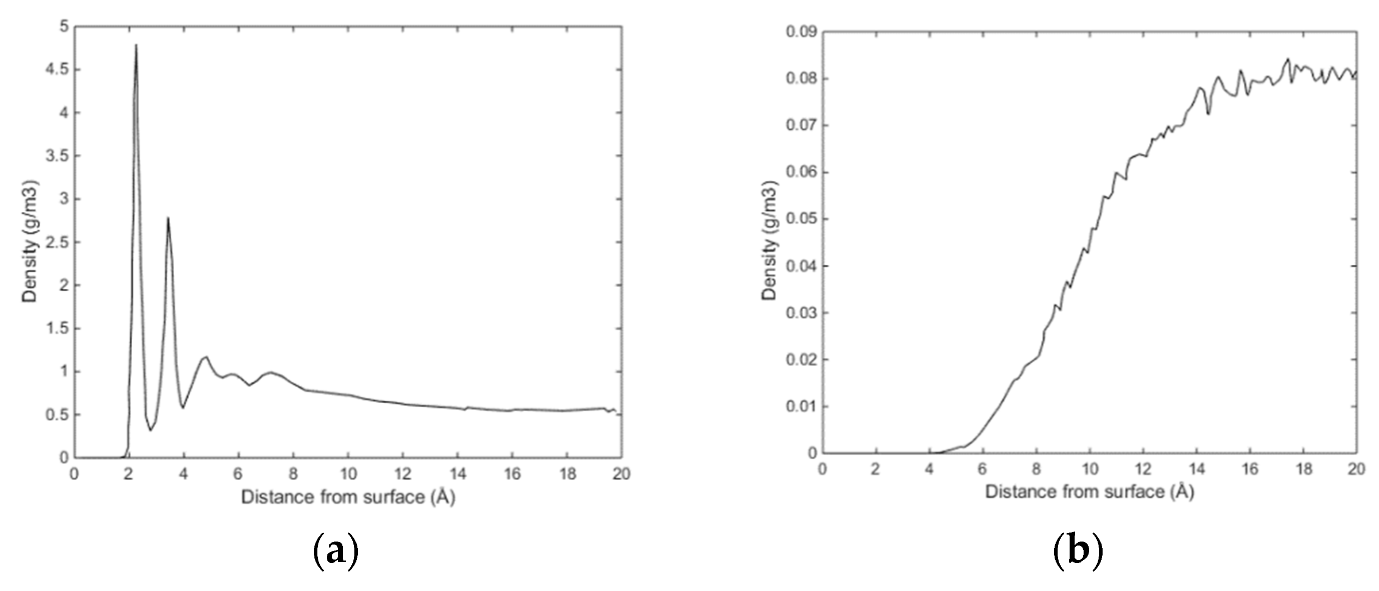
Minerals structure water and lead to extreme densities of the first layers of adsorbed water compared to liquid water densities. We have conducted Molecular Dynamics simulations of water and hydrate formers in contact with various mineral surfaces using LAMMPS [31]. Our recent molecular dynamics studies of water adsorbed on calcite [32] indicate that the density of the first water layer may be as high as 3 times the density of liquid water. Experimental data [33] have a slightly lower first peak for water density but broader peaks. For all practical purposes, like for instance number of nearest neighbours, the agreement between modelling and experimental data is very good. Some polar molecules, like for instance H₂S, adsorb directly on Calcite in competition with water [34,35]. The significant quadrupole moment of CO₂ also leads to direct adsorption on Calcite [36]. Hydrate can therefore form from water outside the Calcite surface where water is close to liquid water in structure, and adsorbed hydrate formers.

However, non-polar hydrate formers, like for instance CH₄, can also be trapped in structured water [36,37,38] and lead to hydrate nucleation when the water is in contact with a separate hydrate former phase [36]. In the absence of a separate hydrate former phase hydrate nucleation like structures are still observed but they dissolve due to low concentration of hydrate formers in water.

Mineral surfaces will therefore act as hydrate inhibitors since hydrate water can never touch mineral surfaces due to the low chemical potential of water in the first adsorbed layers. But mineral surfaces up concentrate hydrate formers through direct adsorption or secondary adsorption in water structures and serve as hydrate nucleation sites. Formed hydrate nuclei can be bridged to the surface of minerals by more or less structured water. A simple model system [36] illustrating the trapping of CH₄ in structured water will be discussed below.

The model system built in [36] comprised several slabs of varying thickness and compositions, with the main ones being calcite and water. A thin phase of methane was introduced between the water phase and the calcite slab on one side, while a thick methane phase was positioned to the other to mitigate the effect of fluctuations on adsorbed methane molecules on the surface due to the volume change of the primary cell. The dimensions of the resulting primary cell for simulation were 39.9 Å × 48.6 Å × 170 Å, and it contained 16,207 atoms.

The crystal structure and all liquid phases were created separately and then combined to build the composite system. MD package LAMMPS [31] was used to implement MD simulations with the time step set to 0.1 fs for the first 1 ps to equilibrate the system. The time step was then increased to 1 fs to achieve equilibrium. During the equilibration run, methane was completely replaced by water on surfaces and thus did not affect the result analysis in this respect. The total equilibration time amounted to 0.501 ns. The production run with the time step increased to 1 fs was conducted for 1.5 ns. An NPT ensemble was emulated, with temperature and pressure (in the z-direction) set to 273K and 100 bar, respectively, via the application of a Nose-Hoover thermostat and barostat. Periodic boundary conditions were applied in all three directions. The L-J potential was used to model the short-range molecular interactions with a cut-off distance of 10 A˚, whereas PPPM was used to evaluate electrostatic interactions. The calcite slab atoms were kept fixed at their crystallographic positions. The forcefield parameters used to calculate the potential energy of the systems can be found in Tables 8.2–8.5 of [36]. The SHAKE algorithm was used to restore the original bond length and angle of water molecules at each time step. Bond and angle potential contributions were included in this simulation based on harmonic style.

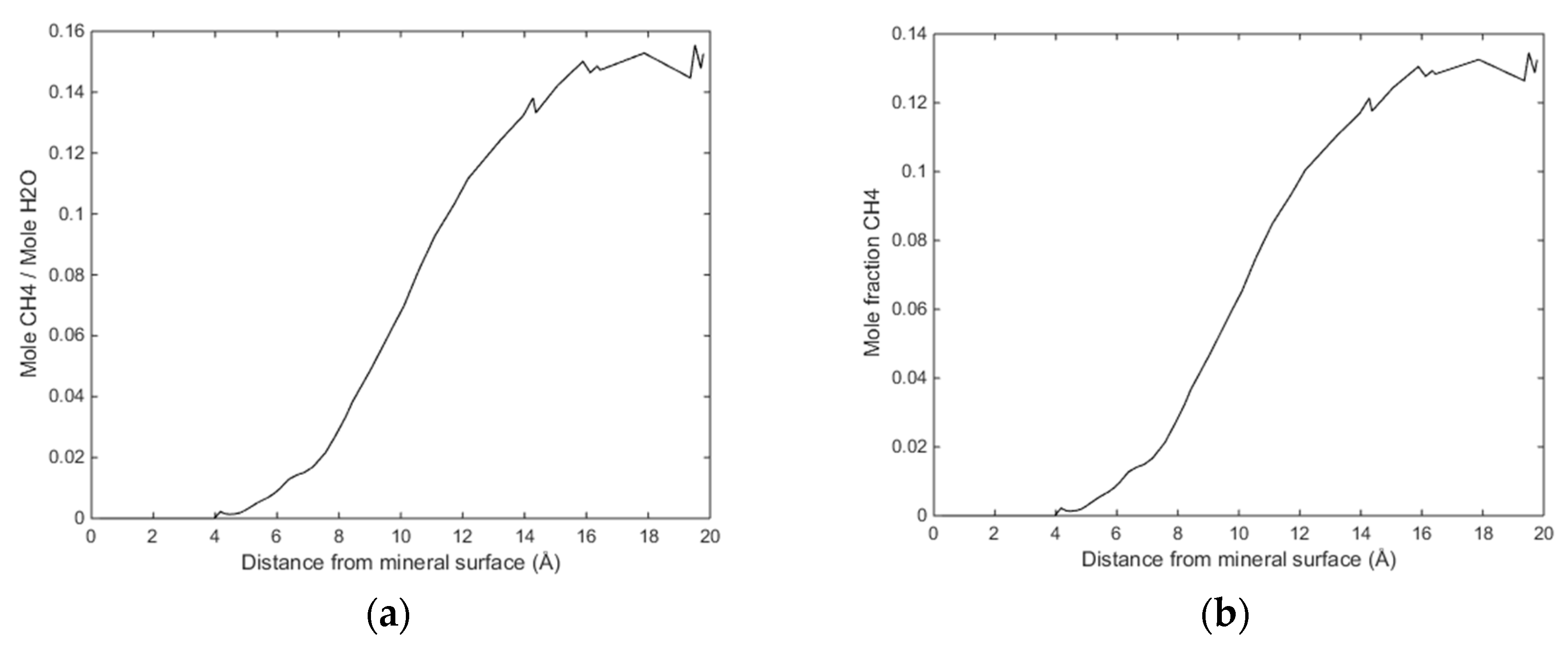
Initially methane adsorbed directly onto the calcite surface despite the absence of partial charges in the one-site L-J model for methane. As simulation progressed, methane and water competed to adsorb on the calcite surface. Water completely replaced methane from the surface since calcite preferred to adsorb water. The water adsorption pattern of the first two layers appeared significantly influenced by the presence of methane, and the time needed to replace the methane completely was about 0.4 ns. The primary layer of water on the calcite-water interface displayed a peak located around 2.28 Å from the surface calcium atom, a distance comparable to the previous experimental and theoretical findings. The next water layer which was still more structured than the water bulk was found at 3.48 Å from the surface. The vigorous interactions between water and the calcite surface can be attributed the strong hydrogen bonding between the two phases. The distance between the first and the second adsorbed layers of water was very small, leaving no space for methane to aggregate. The presence of methane was observed after the second adsorbed layer, with its presence becoming more obvious outside of 6 Å from the calcite surface, as shown in Figure 4 and Figure 5. It was there that the formed methane bubble became trapped, with its location oscillating between 7 and 13 Å from the surface. The methane was not able to escape through the water phase to join the main methane phase within the time span covered in the simulation, with the trapped molecules mainly consisting of those inserted between the calcite surface and the water phase to probe their behaviour under such circumstances. Very few dispersed methane molecules were found in the water phase, as expected from its extremely low solubility. 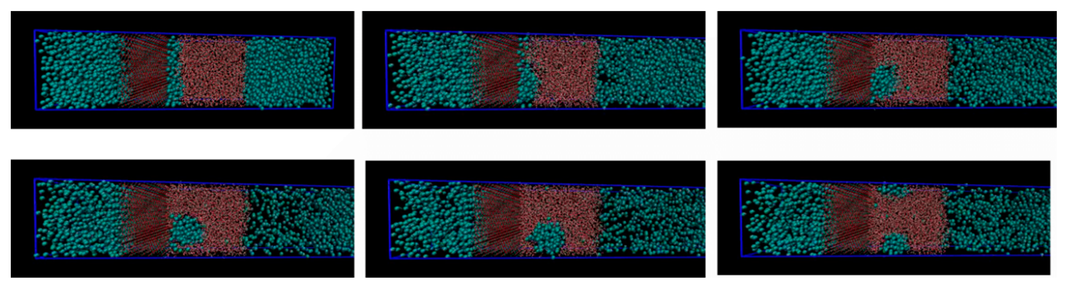Figure 6 traces the time evolution of methane behaviour during the simulation.

The size of the system under study was rather limited, and we are not claiming that the samples in Figure 3 and Figure 4 are representative enough to serve a rigorous nucleation sampling. Larger systems with similar set-up will be investigated in a separate study. The primary information we want to share with these figures is that there are certainly CH₄ trapping effects related to water structures generated by calcite surfaces, and composition of the small nuclei is even close to stable hydrate composition in the centre of the CH₄ accumulations.

4. Pressure Reduction Scenario

Of all the hydrate production methods that have been proposed and examined during the last four decades, pressure reduction has been that examined most in laboratory experiments and pilot plant studies. What is missing in open literature is a more detailed thermodynamic analysis which can shed more light on what is to be expected from this method. Visualization in a pressure temperature diagram does not tell us anything directly about thermodynamic changes. It gives an idea that hydrate can be brought outside stability limits but what are the actual thermodynamic driving forces for dissociating the hydrate, i.e., the free energy change. The second question is: how can the heat of dissociation be supplied in sufficient amounts for commercially feasible production from natural gas hydrates?

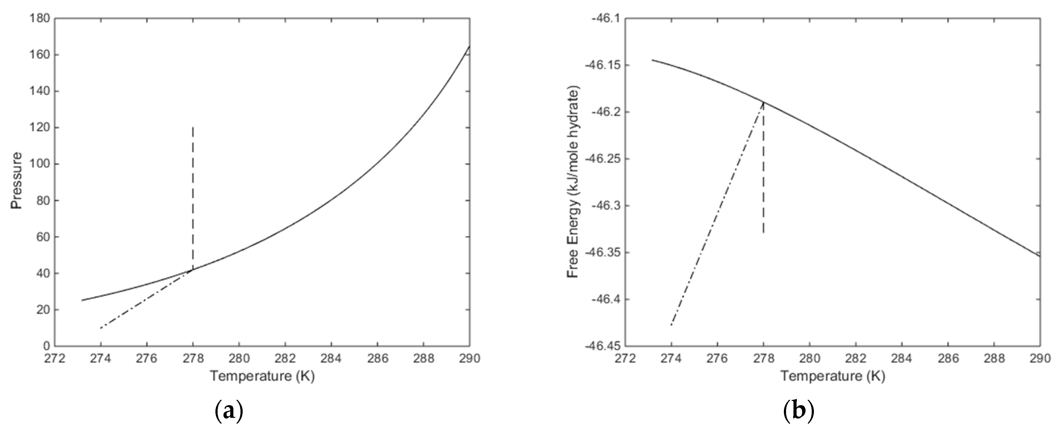
The temperature pressure projection of the stability limits for CH4 hydrate is plotted in Figure 7 below. Temperature, pressure and compositions of all co-existing phases are independent variables while free energy and chemical potentials are the thermodynamic responses of relevance for phase stability and driving forces for phase transitions. The free energy of hydrate formed along the pressure temperature stability limit curve is plotted in Figure 7b. In Figure 7a we also plot in a pressure reduction example scenario. An initial condition of a CH₄ hydrate of 278 K and 120 is reduced to a pressure of 10 bar and 274 K. This is, of course, a very arbitrary example but useful for illustrating two aspects. Pressure reduction on a solid hydrate inside pressure temperature stability zone will not be entirely isothermal since there will be restructuring to lower filling fractions when pressure reduction brings the hydrate down to stability limit pressure. The enthalpy changes related to these processes are expected to be very limited but can be calculated. In Figure 5 this part of the pressure reduction is dashed in Figure 5. Dissociation of the hydrate, and expansion of the released gas, is a kinetic problem that will be discussed separately. At this moment it is simply a dash dot line between the hydrate stability limit pressure and the final condition in Figure 7.

The released gas during pressure reduction from initial condition to stability limit pressure is calculated to 448.63 moles/m³ hydrate. The associated rearrangement of the hydrate involves a limited entropy change. The kinetics of these rearrangements, and the associated gas release, is uncertain and beyond the scope of this work since it will require a set of different fundamental approaches to address. Calculated proeprties of the initial system is given in

Table 2. Properties of initial hydrate and hydrate at stability limit for 278 K.

Properties	T = 278 K, P = 120 Bar	T278, P = 42.05 Bar
Free energy (kJ/mole hydrate)	−46.3288	−46.1894
Filling fraction in large	0.9684	0.9164
Filling fraction in small	0.9502	0.8723
Average MW (Kg/mole)	0.01771	0.01774
Hydrate density (Kg/m3)	911.97	904.79
Molar density (moles/m3)	51,486.4	51,037.8
Gas in hydrate (moles/m3)	7391.54	6942.90

below.

Table 3. Parameters for dimensionless chemical potential functions in Equation (29).

Water Phase, m	a0	a1	a2	a3
Empty structure I	−21.3284	−18.2744	−2.0038	5.2190
Empty structure II	−21.3694	−18.2196	−1.8000	6.2719
Ice (T <273.15 K)	−21.6937	−18.8285	−2.4347	0.1953
Liquid water (T >273.15 K)	−21.6935	−16.2933	−2.0352	3.8636

list proeprties of the water phases for the residual thermodynamic calculation utilized in this work.

Some possible approaches for calculating the phase transition enthalpy changes are given by Kvamme [13,14] and Kvamme et.al. [30,39]. Going back to the original data from the simulations presented in fitted form in the paper by Kvamme and Tanaka [17] an alternative representation of the data can be presented by:

$$\frac{{\mu }_{H_{2}O}^m}{RT}=a_0^m+a_1^m\left[\left(\frac{273.15}{T}\right)-1\right]+a_2^m{\left[\left(\frac{273.15}{T}\right)-1\right]}^2+a_3^m{\left[\left(\frac{273.15}{T}\right)-1\right]}^3$$

(29)

Some other properties along the temperature pressure stability limit curves are also fitted to the same type of function as Equation (29):

$$f(T,P)=a_0^m+a_1^m\left[\left(\frac{273.15}{T(P)}\right)-1\right]+a_2^m{\left[\left(\frac{273.15}{T(P)}\right)-1\right]}^2$$

(30)

Even if the polyonomial is a function of T, every T on the stability limit curve in 4 (a) is an implicit function of the conditions for hydrate P, T stability limit. See

Table 4. Parameters for dimensionless chemical potential functions in Equation (30).

f(T,P)	a0	a1	a2
$G^{Hydrate}(T,P,{\overrightarrow{x}}^{Hydrate})$ (kJ/mole hydrate)	−46.1405	2.5418	−20.5391
$\mathsf{\Delta }{H}^{Hydrate,formation}(T,P,{\overrightarrow{x}}^{Hydrate})$ (kJ/mole hydrate former)	−56.9322	−97.8273	691.3817
Hydrate coordination number (average number of water per hydrate former)	6.4518	6.5428	57.7907

for parameters to Equation (30).

Hydrate dissociates in two different ways. If the kinetic dissociation rate, and the associated release rate of CH₄, is slower than the kinetic rates of dissolving and distributing the released CH₄ in the surrounding water then the free energy change of the dissociation is the free energy change related to the following phase transition:

$${(n{H}_{2}OC{H}_4)}^{Hydrate}\to n{H}_2{O}^{aq.}+C{H}_4^{aq.}$$

(31)

This is at least dominating the initial stages of pressure reduction in which water is dragged in from surrounding parts of the formation. When the dissociation is fast, parts of the hydrate surface will be covered by gas bubbles, as also observed in model studies of CO₂ exchange [2,3,6]. In both cases the hydrate dissociation will lead to a continuous replacement of the hydrate/liquid water interface. The difference is therefore essentially that the dissociation rate is higher for regions of direct contact between hydrate and liquid water. Regions covered by gas bubbles will involve that the water driving force is sublimation into gas bubble while CH₄ driving force is difference in chemical potential between CH₄ in hydrate and CH₄ in gas bubble. In both cases, hydrate and water will continuously redevelop a new interface. The transport of CH₄ through the interface layer will therefore be the same in both cases. Unlike nucleation of hydrate particles during formation there will as such not be the penalty of pushing away old phases during hydrate dissociation. But the free energy driving forces are different.

$${(n{H}_{2}OC{H}_4)}^{Hydrate}\to n{H}_2{O}^{aq.}+C{H}_4^{gas}$$

(32)

Calculated free energy change for this phase transition in our example is then −0.24 kJ/mole hydrate. The corresponding Boltzmann factor for thermodynamic control of the phase transition in Classical nucleation theory is then 1.10. The maximum thermodynamic driving force for the phase transition according to (32) at initial temperature and stability limit pressure is −0.05 kJ/mole. The associated Boltzmann factor is 1.02. In simple Classical Nucleation Theory (CNT) then the combined mass transport and thermodynamic control is:

$$J=J_0{e}^{-\beta \mathsf{\Delta }{G}^{}}$$

(33)

where J₀ is the mass transport flux for the dissociation. A model for the transport across the hydrate water interface was proposed by Kvamme et.al. [15] based on samplings from molecular dynamics simulations. Using this model, and a simple mass transport calculation, showed that is was possible to predict induction time for CH₄ hydrate in an experimental plastic cell [9,15]. See Equation (31) below and associated parameters in

Table 5. Parameters for Equation (34).

I	Parameter	i	Parameter	I	Parameter
1	0.979242	4	171.673	7	−9649.96
2	15.5427	5	6.76975	8	14,779.7
3	−88.5112	6	1939.55	9	−7496.15

. For CH₄ we use D_liquid equal to 5·10⁻⁸ m²/s.

$$\left[\frac{D{(z)}_j}{D_{liquid,j}}\right]=9.5\cdot {10}^{-{\displaystyle \sum _{i=1}^9{a}_i{\left(a\tan \left[(0.5z\frac{\pi }{2})/12\right]\right)}^{i-1}}}$$

(34)

Calculated critical radii for CH₄ hydrate at two different temperatures are given in Figure 3a. The associated nucleation times are based on integration of Fick’s law:

$$t(R=12\AA )-t(R=0\AA )={\displaystyle {\int }_{C_{C{H}_4}(R=0)}^{C_{C{H}_4}(R=12)}\frac{\partial C_{C{H}_4}(z)}{\left[-D_{C{H}_4}(z)\frac{{\partial }^2{C}_{C{H}_4}(z)}{\partial z^2}\right]}}$$

(35)

The concentration profiles for CH₄ as a function of distance from the hydrate side of the interface to the liquid side of the interface is available from Kvamme [13,14] and Kvamme et.al. [28]. The diffusivity coefficient profile for CH₄ is given by Equation (34), with parameters from Table 5. For 280 K and a stability limit pressure Figure 7a of 42.05 bar the enthalpy of hydrate dissociation is calculated to 55.0 kJ/mole guest for CH₄ hydrate. The calculated dissociation flux based on Equation (32) is 2.54 × 10⁻⁵ moles CH₄/m²·s for a CH₄ concentration in surrounding water close to the hydrate stability concentration in Figure 2b. In practice, the capacity of the surrounding water to distribute released CH₄ in water solution is the difference between Figure 2a and the concentration projection of Figure 3a. The associated mass transport limited heat needed is therefore 1.40 × 10⁻³ kW/m². The thermodynamic impact is calculated to range between 1.02 and 1.10 as discussed above. Using 1.10, then the heat flux needed to support transporting guest molecules from hydrate and dissociate the hydrate is 1.54·10⁻³ kW/m². Note that these example values reflect guesses of a situation related to dynamic pressure reduction production, in which it is expected that background CH₄ content in water surrounding the hydrate is high and other factors also reduce dissociation flux according to driving for between chemical potential of CH₄ in hydrate and CH₄ in surrounding liquid water. This is just an example used to illustrate that the drawback of pressure reduction is that the method does not address a kinetic bottleneck of transporting molecules across a water hydrogen bonded interface. This is in contrast to thermal stimulation and adding chemicals that breaks water hydrogen bonds.

For comparison of the span of hydrate dissociation fluxes that can be present, the maximum value of dissociation fluxes calculated in the example related to hydrate dissociation.

The estimated dissociation fluxes above, therefore, are smaller than those in the next section which are estimations of dissociation fluxes of hydrate in contact with inflow of water through fracture systems.

With the approximation of heat transport being represented by an “efficient” heat conductivity then Fourier’s law is generally given by:

$${\dot{Q}}_{conductivity}=k\nabla T$$

(36)

where the heat conductivity will vary during a production scenario. Hydrate saturation (volume per cent hydrate in pores) varies. But even in very closed reservoirs, like in permafrost regions in Alaska, it is hard to find any saturations higher than 85% and 75% as more typical. Offshore hydrates have generally lower hydrate saturations due to imperfection is sealing structures. Fracture systems that bring in seawater will lead to hydrate dissociation due to low content of CH₄ in the incoming seawater, according to the stability limits in Figure 2a.

Heat conductivity will vary during hydrate production as the hydrate saturation gradually decreases. Heat conductivities that range from sediments with high hydrate saturation down to same sediments filled with liquid water are relevant for modeling purposes. But in a bigger picture it is also of interest to evaluate heat conductivities for liquid water, hydrate and sediments separately for the purpose of developing new theoretical models for heat conductivities in these systems of solid material and various water phases. Compared to heat conductivity in other phases, gas is a heat insulator and in a relative sense can often be approximated with zero heat conductivity.

Geo thermal gradients provide an initial temperature gradient from the top of a hydrate filled section down to the inlet of a production pipeline, whether this is a vertical completion or some version of horizontal completion. An additional temperature gradient will establish due to Joule–Thomson effects. These effects are very unique for each reservoir and for various stages of a production scenario. As such, it is not possible to develop some general conceptual correlations for this since it is a complex implicit dependency of mass and heat flow as well as dynamics of phase transitions. In general, a capable hydrate reservoir simulator can address this, provided that the simulator has sufficient rigorous treatment of thermodynamics and non-equilibrium phase transitions.

A simple one dimensional model of Fourier’s law can be used for a qualitative analysis of the relative heat transport.

$${\dot{Q}}_{conductivity}=k\frac{dT}{dz}$$

(37)

In which the unit of the thermal conductivity k is W/m·K. An interesting ratio is, therefore, the heat needed by the mass transport limited process of transporting guest molecules from hydrate to surrounding phases:

$$q_r=\frac{{\dot{Q}}_m}{{\dot{Q}}_{conductivity}}=\frac{J\mathsf{\Delta }H}{k\frac{dT}{dz}}$$

(38)

Heat conductivity is of course not the only way that heat is transported in a porous media but experimental data on heat transport in hydrate filled sediments is often approximated into a “lumped” heat conductivity coefficient. Similar for heat transport in hydrate reservoir simulators, which are frequently modelled as heat conductivity, with correlation for estimating heat conductivity from the pore filling volume fractions of the various phases, and the respective heat conductivities in these phases. For condensed phases these heat conductivities do not vary much with pressure. For liquid water the variation with pressure is practically zero while there is a very limited variation for hydrate due to the pressure dependency in filling fractions. This hydrate pressure dependency for heat conductivity is not very significant for non-polar guests but slightly higher for polar guest molecules like, for instance, H₂S. In a pore scale model for heat conductivities during production there is of course also a need for heat conductivities for the gas phase. There are ways to calculate these but that is outside the scope of this paper. In many cases it would even be a fair approximation to approximate heat transport through gas as zero compared to the relatively high heat transport capability of minerals and water phases. On a larger scale there are hydrate-filled reservoirs that contain significant local volumes of separate hydrate phase. These types of reservoir hydrate fillings can typically build up as function of a balance between fractures that leads water into the hydrate sections from the ocean (vertically, horizontally and all possibilities in between), and fracture systems that bring in hydrate formers from below. Concentration of hydrate formers in incoming water is normally close to zero and in situ hydrate will therefore dissociate according to the stability limit window illustrated in Figure 3a. In certain cases of the balance between hydrate dissociation and formation of new hydrate the local flux inflow of gas may be large enough for the new hydrate to push aside sand and create hydrate filled “pockets” outside pore-filling hydrates. In

Table 6. Heat conductivities, k, for various transport media with water in units of W/mK φ is porosity. C is average mineral composition (when available) in terms of relative portion of well-defined minerals, or in terms of average atomistic composition. R denote specific remarks, in which E denote experimental values and M denote theoretical values used in modeling. Missing information is denoted by N/A. In the T, P columns specific temperatures are in Celsius and pressures are in MPa. For references that report several different conditions and/or gradient information the letter S is used and reader is directed to the original reference for details.

Minerals	C	Φ	T	P	k	R	Ref.
Quartz sand	N/A	0.442	6.12	4.50	1.0	E, M	[41]
			6.02	4.50
			5.14	4.50
			3.89	3.50
			7.78	5.50
A porous medium	N/A	0.3	S	S	2.0	M	[42]
Porous shale	N/A	N/A	S	S	1.0	M	[42]
Bentheim sandstone	95%−99% quartz content with traces of the clay mineral kaolinite	0.23	4.00	3.96	0.5	E, M	[43]
			4.00	3.89
			4.00	3.82
Calcite and quartz	3.6% calcite, 86.4% quartz in aquifers	0.1	S	S	4.64	M	[44]
	4% calcite, 95% quartz in caprocks	0.01
	3.8% calcite, 91.2% quartz in fracture	0.05
Quartz	N/A	0.3 in aquifer	S	S	0.5	M	[45,46]
		0.03 in cap rock
		0.5 in fracture
Granite	TiO2, Al2O3, MgO, FeOT, CaO, P2O5, K2O and 66.4–75.0% SiO2	Varies from 0.511–2.636%	25	0.1	2.12–3.12	E	[47]
Sandstone-1	N/A (1)	5%	0–150	0.1	1.82–2.01	E	[48]
Limestone	N/A (2)	5%	0–150		1.55–1.94
Amphibolites	N/A (3)	1%	0–150		2.35–3.52
Granulate	Saxonian Granulate Mountains, Germany, quartz 38%, pla-gioclase 9%, K-feldspar 47%, biotite 1%, 4% granite, mixture of crystalline and amorphous structures	1%	0–150		1.77–2.06
Pyroxene-granulate	Saxonian Granulate Mountains, Germany, granite 6%, clinopyroxene 39%, plagioclase 34%, non-transparent minerals 11%, orthopyroxene 9%, ambibolb1%	1.2%	0–150		2.40–2.46
Siltstone	N/A (4)	1%–2%	2–250		1.93–2.62
Dolomite	N/A (5)	1%–2%	2–250		3.14
Sandstone-3	N/A (6)	13%	2–250		2.34–2.71
Quartz	N/A	N/A	N/A	N/A	7.7	E	[49]
Feldspar					2.3
Pyrite					19.2
Calcite					3.3
Dolomite					5.3
Anhydrite					6.3
Chlorite					3.3
Kaolinite					2.9
Smectite					1.9
Illite					1.8
Illite/smectite					1.8

Notes: All dry mineral thermal conductivity data are measured when air is filled in a porous medium. There is no paper measuring thermal conductivity in vacuum environment in the above table. The values of T and P are not all the environmental conditions for measuring thermal conductivity, some of which are the temperatures for the related hydrate experiments in these papers. 1. Aktash, Dagestan, Russia, borehole #1, 2977 m. 2. Soltangasha, Dagestan, Russia, borehole #96, 201 m. 3. Kola ultra-deep borehole, 10,000 m. 4. Dmitrievskoe, from oil-gas field, borehole #D44, Dagestan, Russia, 4570–4574 m. 5. Dmitrievskoe, from oil-gas field, borehole #D44, Dagestan, Russia, 4247–4248 m. 6. Solonchak, Dagestan, Russia, borehole #34, 3941 m.

and

Table 7. Heat conductivities, k, for various transport media with water in units of W/mK. φ is porosity. C is average mineral composition (when available) in terms of relative portion of well-defined minerals, or in terms of average atomistic composition. x is liquid water composition. In some cases the listed value is an average composition and denoted in brackets. R denote specific remarks, in which E denote experimental values and M denote theoretical values used in modeling. Missing information is denoted by N/A. In the T, P columns specific temperatures are in Celsius and pressures are in MPa. For references that report several different conditions and/or gradient information the letter S is used and reader is directed to the original reference for details.

Minerals		C	φ	T	P	x	k	R	Ref.
Quartz sand		N/A	0.442	6.12	4.50	<0.274>	2.1	E, M	[41]
				6.02	4.50
				5.14	4.50
				3.89	3.50
				7.78	5.50
A porous medium		N/A	0.3	S	S	N/A	2.18	M	[42]
Porous shale		N/A	N/A	N/A	N/A	S	3.1	M	[42]
Construction sand with quartz as the primary component		N/A	0.47	0	6.6	N/A	2.08	E, M	[46]
Bentheim sandstone		95%−99% quartz content with traces of the clay mineral kaolinite	0.23	4.00	3.96	0.45	3.1	E, M	[43]
				4.00	3.89	0.50
				4.00	3.82	0.44
Calcite and quartz		3.6% calcite, 86.4% quartz in aquifers	0.1	S	S	N/A	2.64	M	[44]
		4% calcite, 95% quartz in caprocks	0.01
		3.8% calcite, 91.2% quartz in fracture	0.05
Quartz		N/A	0.3 in aquifer	S	S	0.5	0.5	M	[45,46]
			0.03 in cap rock
			0.5 in fracture
Granite		TiO2, Al2O3, MgO, FeOT, CaO, P2O5, K2O and 66.4–75.0%SiO2	Varies from 0.511–2.636%	25	0.1	Varies from 0 to 1	2.99–3.62	E	[47]
Sandstone-2		N/A (1)	16.2%	2–150	0.1	N/A (water saturated sand	2.25–2.30	E	[48]
Sandstone-3		N/A (2)	13%	8–245	0.1		3.41–3.81
Mudstone	Tertiary mudstones	sandy mudstones, claystones (26%–50%) andquartzite, clayey (16–45%)	N/A (can calculated by the water content)	22–38	0.1	9%–42%	0.79–1.14	E	[49]
	Sandy siltstone	Quartz (13%–21%), feldspar and micain a clayey matrix (50%–70%).				11%–19%	0.71–1.02
	fissile mudstones	clay (30%)quartz (42%)				21%	0.92 and 1.04

Notes: Some papers on hydrate do not give the thermal conductivity at different temperature and pressure, but use the same value. 1. Buinaks, Dagestan, Russia. 2. Solonchak, Dagestan, Russia, borehole #34, 3941 m.

we list some values for heat conductivities of various heat transport nedia containing water. Real sediments in real pilot plant experiments, like for instance the Ignik Sikumi [40] there is a variety of mineral types. In the long run we need to develop new correlations for heat transport through mixed media contining minerals, hydrate, liquid water and gas. For that reason we also list properties of water as well as dry minerals. See

Table 8. Heat conductivity for liquid water (W/mK) [50]. Temperature in K.

T	k
274.15	0.5587
275.15	0.5609
276.15	0.5631
277.15	0.5653
278.15	0.5675
279.15	0.5697
280.15	0.5718
281.15	0.5739
282.15	0.5760
283.15	0.5781
284.15	0.5801
285.15	0.5821
286.15	0.5841
287.15	0.5861
288.15	0.5881
289.15	0.5900
290.15	0.5919

$T^{*}=T/298.15$, $k^{*}=k(T)/k(298.15)$, $k(298.15\mathrm{K},0.1\mathrm{MPa})=0.6065\pm 0.0036W{\mathrm{m}}^{-1}{\mathrm{K}}^{-1}$, $k*=-1.48445+4.12292T*-1.63866T^{*2}{}_{}fo{r}_{}274\le T\le 370\mathrm{K}$.

and

Table 9. Heat conductivity for hydrate as separate phase without sediments. T, P columns specific temperatures are in Kelvin and pressures are in MPa.

P	T	k	Ref.
4.0	263.2–283.1	0.4846–0.4953	[51]
6.0	263.2–279.2	0.4851–0.4946
9.5	263.2–275.3	0.4866–0.5467
6.6	273	0.575	[46]
0.2	216	0.45	[52]
6.6	263.06–277.87	Uncompacted, 0.334–0.381	[53]
		Compacted, 0.568–0.587
3.8–14.2	261.5–277.4	<0.68 ± 0.01>	[54]
31.5	−20–15	0.62 ± 0.02	[55]

for heat conductivities of various individual phases/media involved. Some typical values of relevant geothermal gradients are listed in

Table 10. Geothermal gradients.

Temperature Gradient (K/m)	R	Ref.
0.019	water depth of 1344 m	[56]
0.0355	/	[42]
0.03	/	[42]
0.019 ± 0.002	at site 17, water depth 1150 to 1350 m, depth below seafloor range from 0 m to 700 m	[57]
0.090–0.110	Water depth range from 898 m to 2153 m	[58]
0.04753; 0.04695; 0.04934; 0.06760; 0.04365	5 sites, water depth range from 1105 m to 1290 m	[59]
0.055	a total depth of 1225 m:1000 m water depth, 225 m sediment depth	[60]
0.04; 0.032; 0.02	permafrost, in different possible depth	[61]
0.035 (in the model); 0.043; 0.03; 0.036	HBL of the Shenhu area, L-Pad area, the Prudhoe Bay, in the Mt Elbert area	[62]
0.036	used in model	[45]

.

Some illustrations of Equation (38) is given in

Table 11. Relative heat transport rates q_r for various transport mediums and various temperature gradients and some typical values for various media. All k-values in W/m·K.

Transport Medium	qr for Various Temperature Gradients
	$\frac{\mathit{d}\mathit{T}}{\mathit{d}\mathit{z}}=0.04\mathbf{K}/\mathbf{m}$	$\frac{\mathit{d}\mathit{T}}{\mathit{d}\mathit{z}}=0.07\mathbf{K}/\mathbf{m}$	$\frac{\mathit{d}\mathit{T}}{\mathit{d}\mathit{z}}=0.09\mathbf{K}/\mathbf{m}$	$\frac{\mathit{d}\mathit{T}}{\mathit{d}\mathit{z}}=0.12\mathbf{K}/\mathbf{m}$	$\frac{\mathit{d}\mathit{T}}{\mathit{d}\mathit{z}}=0.15\mathbf{K}/\mathbf{m}$
Liquid water, k = 0.56	0.022400	0.039200	0.050400	0.067200	0.084000
Hydrate, k = 0.49	0.019600	0.034300	0.044100	0.058800	0.073500
Water filled sediments, k = 2.7	0.108000	0.189000	0.243000	0.324000	0.405000
Hydrate filled sediments, k = 2.5	0.100000	0.175000	0.225000	0.300000	0.375000

based on some average values from Table 8 to Table 9.

5. The Use of CO₂

As also discussed above, one of the critical limitations of the pressure reduction method is the lack of sufficient heating of the interface. Slow diffusion of CH₄ though the water/hydrate interface is a dynamic bottleneck in dissociation of the hydrate. Any thermally based method is kinetically efficient because of the breaking of hydrogen bonds and loosening up of the hydrate/water interface structure. Direct addition of heat in the form of steam or hot water is not economically feasible. Other ways of adding heat has also been proposed but still remain to be proven economically and technically feasible. Other ways to break water hydrogen bonds are also well known from hydrate inhibition. Methanol is likely the most used thermodynamic hydrate inhibitor but any chemicals and salts that break hydrogen bonds will do the work of hydrate dissociation. But the cost is beyond any realistic economic feasibility relative to value of produced gas from hydrate.

Another alternative, which is often misunderstood, is the use of CO₂. Several research groups around the world have spent several years experimenting on the injection of CO₂ into hydrate filled sediment models in laboratories. Few of these have been successful because injected CO₂ will result in nucleation of new hydrate with the free water in the pores. These nucleation processes happens on a nano second time scale [13,14,15] (and references in these papers). This will rapidly lead to blocking of the sample and to extremely slow conversion from in situ CH₄ hydrate to CO₂ hydrate.

As a possible way to reduce this blocking the addition of nitrogen has been utilized by some research groups. Addition of N₂ was also utilized in the Ignik Sikumi pilot plant test [1,40]. Limited amounts of N₂ in CO₂ will still make it possible to create new CO₂ dominated hydrate together with free pore water. Another positive effect of adding limited amounts of N₂ is the increase in gas permeability for the CO₂/N₂. However, N₂ does not address the limitation of hydrate films and additional chemicals are needed to keep the water/CO₂ interface hydrate free. The theoretical study of Kvamme et. al. [28] provides some insight into how surfactants promote hydrate formation without blocking water CO₂ interface. The most feasible mechanism for in situ CH₄/CO₂ swap does not actually involve direct contact with the CH₄ hydrate. Formation of a new CO₂ hydrate releases excess heat compared to necessary heat for CH₄ hydrate dissociation [13,14,30]. This is also consistent with model studies using Phase Field Theory [2,3], which demonstrate a liquid water mass transport limited kinetic rate as long as free water is available around CH₄ hydrate core. This liquid transport controlled process changes to a slow solid state controlled exchange when the free water is consumed. As also discussed by Kvamme [1] the high N₂ content in the injection CO₂/N₂ gas mix used in the Ignik Sikimu [1,40] might be an important reason for the limited efficiency observed in the pilot test.

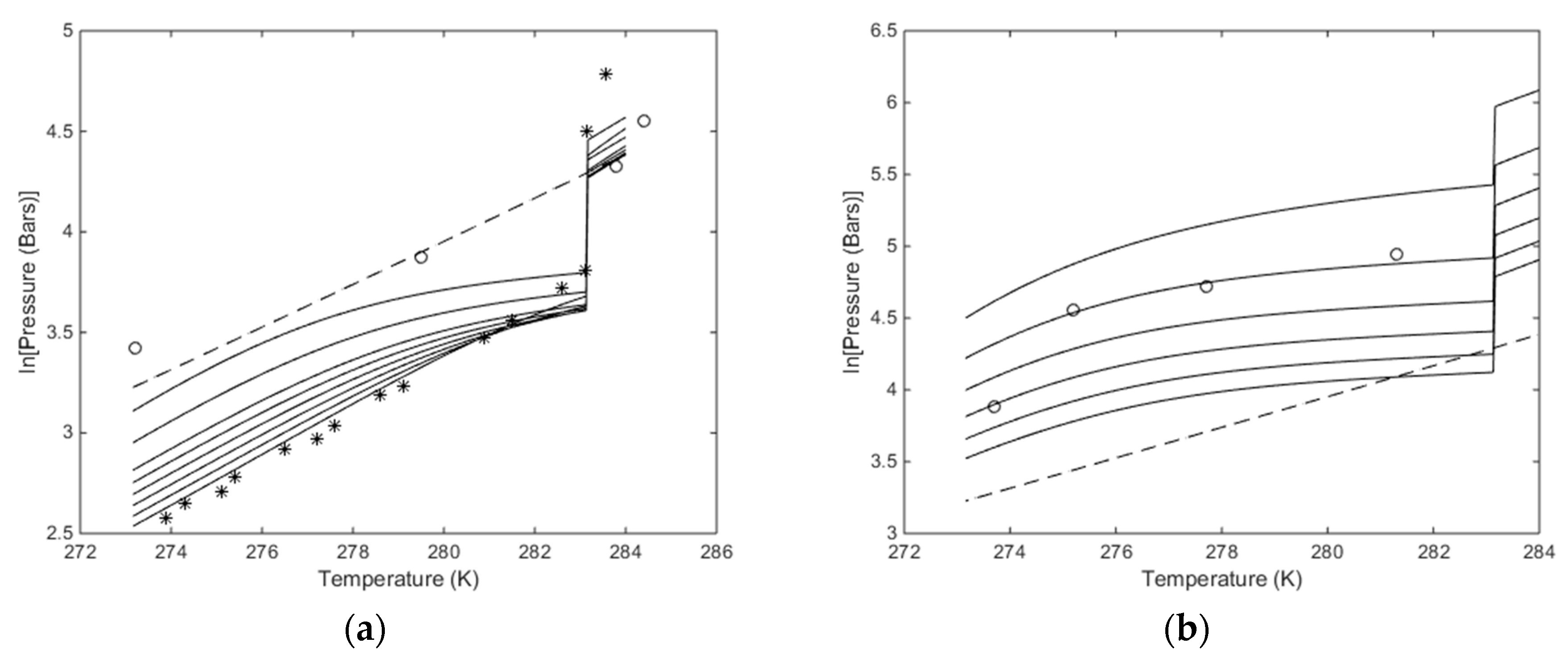
Plots of stability limits in independent thermodynamic variables do not tell us anything about feasibilities in terms of energy, but since chemical potential of water and hydrate formers are used for constructing pressure temperature stability limits then Figure 8 and the comparison with experimental data give some model verification. Figure 8b is the most interesting in terms of using CO₂/N₂ mixtures. Although it does not tell anything about the energies involved and the possible feasibility of using these mixtures less than 30% CO₂ may not be feasible. But as discussed above, the free energy change has to be feasible enough to facilitate the phase transition. And sufficient heat must be available to support the needed enthalpy of dissociation for the hydrate. 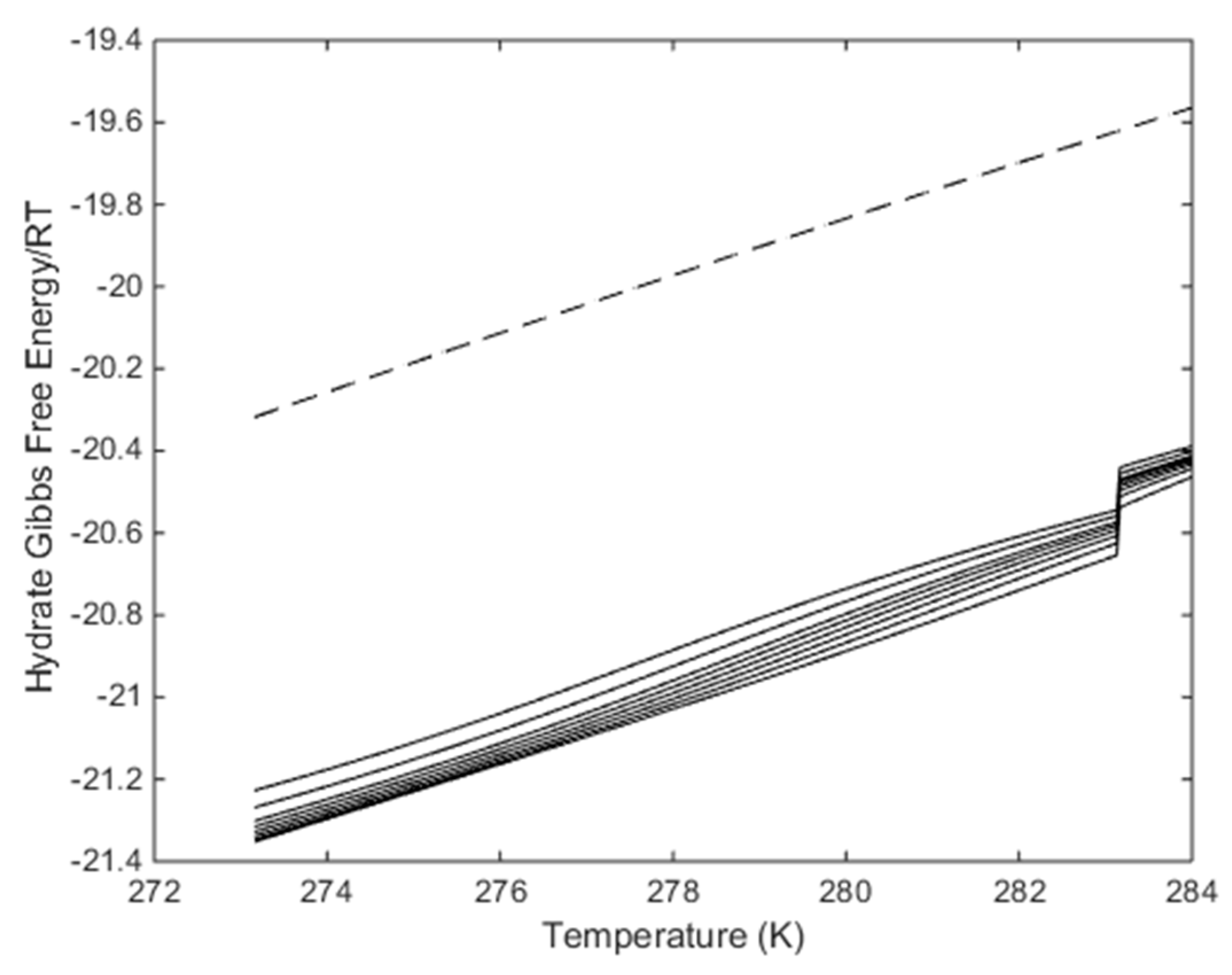In Figure 9 we plot the free energy changes associated with the hydrates along the curves in Figure 8b.

Figure 9 tells us that the formation of a new hydrate from injection gases with composition in the range of the CO₂/N₂ plots in Figure 9 will be more stable the in situ CH₄ hydrate at same conditions. But Figure 9 does not tell if these phase transitions are possible in terms of all independent thermodynamic variables in the system. Since water is the dominating component than a first check would be to find out the maximum N₂ content for which hydrate water chemical potential is lower than liquid water chemical potential. This has already been done by Kvamme [1] and CO₂ less than roughly 25 mole% in CO₂/N₂ mix is unlikely to make a new hydrate with free pore water. There is, however, another point that can make it possible to make hydrate from even more dilute mixtures. As also discussed by Kvamme [1], there will be selective adsorption of CO₂ on the surface of liquid water prior to hydrate formation. i.e., the concentration of CO₂ on the gas/water interface is likely to be significantly higher than the average gas concentration of CO₂. Based on calculations of selective adsorption [1] of CO₂ from CO₂/N₂ mixtures as pre-stages for hydrate formation, even CO₂/N₂ mixtures up to 35 mole% N₂ might be feasible. However, this also depends on low dosage additives that can keep the water/gas interface free of blocking hydrate [28].

The considerations above are entirely based on aspects related to free energy changes and chemical potential driving forces for phase transitions. The second aspect on the feasibility of CO₂/N₂ and maximum percentage nitrogen is the associated needed heat for dissociation of the CH₄ hydrate. Based on earlier studies [14,30] it is known that the excess heat available from formation of hydrate from pure CO₂ hydrate is in the order of 10 kJ/mole more than what is needed for dissociation of the in situ CH₄ hydrate. The question is how added N₂ changes the enthalpy of hydrate formation.

For this purpose we can examine specific cases of temperature and pressure. A first example is illustrated in Figure 8, Figure 9 and Figure 10 below. Calculations are performed for a temperature of 274 K and 170 bars pressure. Note that pure CO₂ is not able to fill the small cavity of structure I at liquid water conditions. There is some evidence that CO₂ also can get trapped in small cavity at very low temperatures [65] but so far we have no evidence of CO₂ filling in small cavities at liquid water hydrate-forming conditions. According to our studies using methods from classical statistical mechanics and quantum mechanics, we do not see any possibility for CO₂ to stabilize the small cavity. This is important for the evaluation of changes in hydrate stability limits when N₂ is added. The addition of N₂ changes the chemical potential of CO₂ in the mixture. 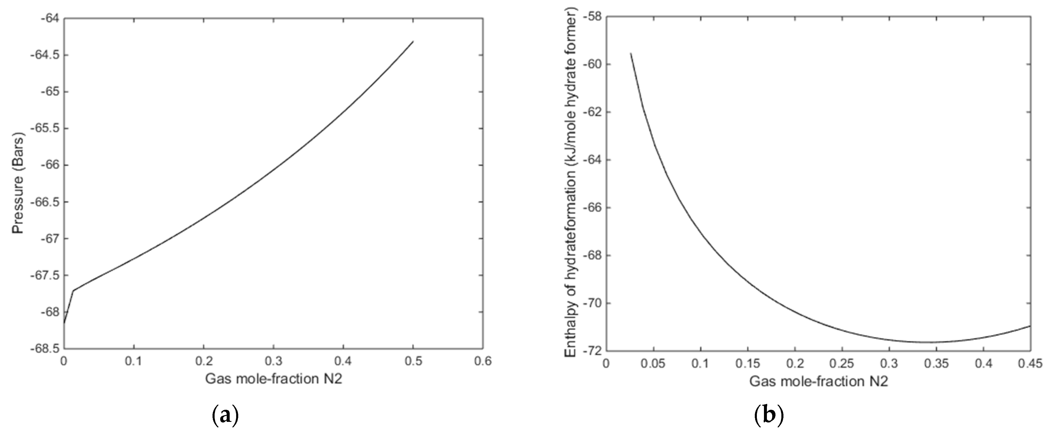On the other hand, N₂ entrance in small cavities adds to the hydrate stability. In Figure 10 we plot the stability limit pressures for 274 K (Figure 10a) and stability limit temperatures for 170 bars pressure (Figure 10b). In Figure 9 we plot the enthalpies of hydrate formation as function of filling fractions for a pressure of 170 bars along the stability limit temperatures in Figure 10b.

The most relevant of these figures are Figure 8a and Figure 9a, although the transport of heat from forming CO₂/N₂ hydrate will lead to local temperature increase and consumption of heat for dissociation of CH₄ hydrate.

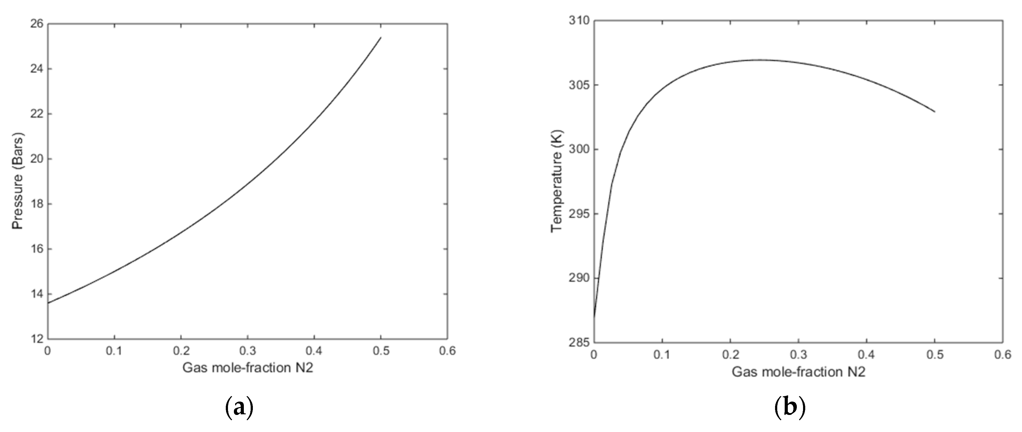
With reference to Figure 11b there is no change in gradient for the small fractions of N₂. It is just an artefact of the applied resolution in that end of the mole-fraction N₂. With a finer grid in that end it will show a smooth curve. The relevant information from Figure 11a is that even for a gas mixture of 30% N₂ there is enough excess heat to dissociate in situ CH₄ hydrate. The available excess heat; heat released from formation of hydrate from injection gas as compared to heat needed to dissociate CH₄ hydrate, is reduced from roughly 10 kJ/mole hydrate former down to roughly 8 kJ/mole. As compared to low temperature heat in the pressure reduction method this is substantial since the heat is directly generated in the pores during formation of the new hydrate.

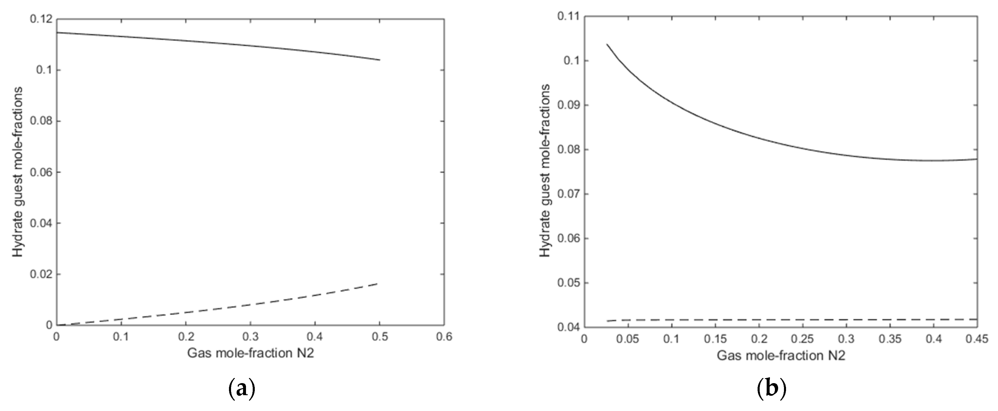
A final figure for this first example is the mole-fractions of guest fillings in the hydrate for the two cases in Figure 12a,b.

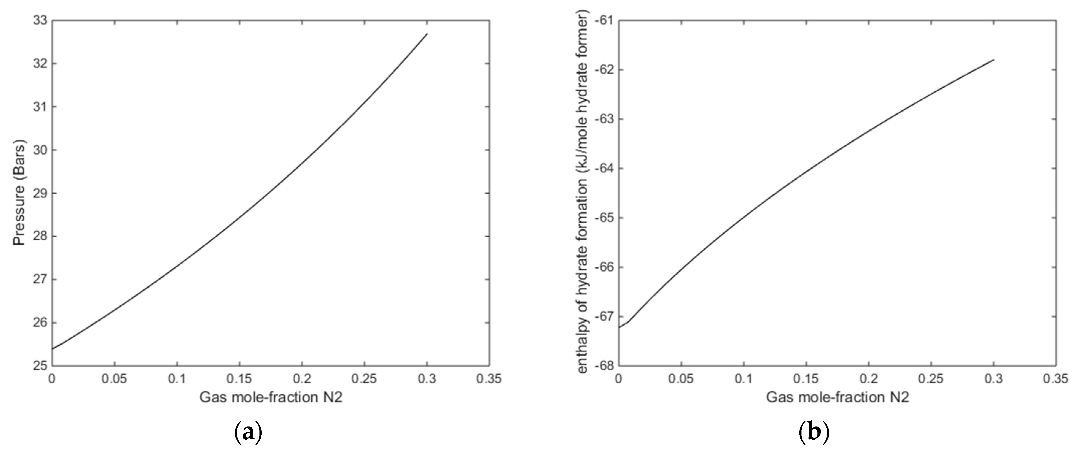
In Figure 13, we plot stability limits pressure for 279 K as function of mole-fraction N₂ in the gas, and associated enthalpies of hydrate formation. Also for this temperature there is sufficient available released heat form hydrate formation to ensure CH₄ hydrate dissociation.

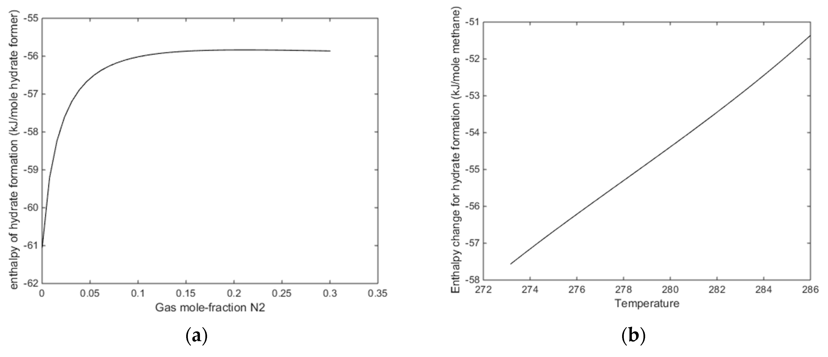
The more critical question is what happens when the temperature is reached at which pure CO₂ would undergo a phase transition. From Figure 6 and Figure 7 we know that this transition temperature for CO₂ will also affect CO₂/N₂ mixture properties. In Figure 14a we plot enthalpies of hydrate formation as function of mole-fraction N₂ along pressure stability limits for 284 K. In Figure 14b, we plot enthalpies of hydrate formation for CH₄ hydrate as function of temperature, along the pressure temperature stability limits. Comparing the values from Figure 14a with the enthalpies of CH₄ hydrate formation at 284 K for 284 K, it can be observed that there is still a net difference between formation of hydrate from CO₂/N₂ mixture, and formation enthalpy for CH₄ hydrate in the order of 4 kJ/mole hydrate former [14].

6. Offshore Hydrates, Pockmarks and Relevance for Hydrate Production

As discussed elsewhere, hydrate in sediments are not generally stale in sediments. They reside in a stationary balance between inflow of new hydrocarbons through fracture systems from below, which generates new hydrate, and inflow of seawater trough fracture systems which leads to hydrate dissociation according to Figure 3a. The tighter the sealing (clay, shale) of the hydrate section, the higher the hydrate saturation if the supply of hydrocarbons is sufficient.

From a hydrate production point of view this is interesting for two reasons. The first of these is that the average hydrate saturation is highly dependent on the distribution of fracture systems that results in inflow of seawater into the hydrate-filled sections, and the associated flux rates. The second reason is that pressure reduction does not result in high enough temperatures to break the hydrogen bonded structure of the interface, as discussed earlier. Dissociation of hydrate in chemical potential gradients of hydrate guest molecules is, therefore, a significant dissociation mechanism for the hydrate during pressure reduction method for hydrate production.

In many cases the number of pockmarks and associated methane leakage fluxes can be the first indicator of the dynamics of the hydrate system. And frequently it is so that a high number of pockmarks that leaks methane indicate low average hydrate saturation and corresponding limited commercial value. One example is the Nyegga area offshore Norway, for which the average hydrate saturation is estimated to vary between 7% and 15% [66,67] (and references in these). An example from offshore China is reported by Luo et al. [68], which is very detailed in geochemical analysis, and corresponding estimates of methane fluxes. This study does not, however, contain enough information to estimate hydrate saturations and methane hydrate production potential.

Unlike pressure reduction hydrate production the background CH₄ concentration in the water that leaks in to hydrate-filled sediments through fractures are expected to have a fairly low CH₄ concentration. The salinity of pore water surrounding the hydrate may be different from incoming salinity. The initial CH₄ in the water surrounding hydrate in the pores is very sensitive to the dynamic situation of the reservoir, i.e., dynamics of new hydrate formation and dynamics of hydrate dissociation. For the purpose of this paper, and in the absence of detailed data for specific cases, we just illustrate the sensitivity of hydrate dissociation fluxes on background concentration of CH₄ and diffusivity on hydrate side of the interface. Some example values are listed in

Table 12. Calculated hydrate dissociation fluxes in gradients of chemical potentials between CH₄ in hydrate and CH₄ in surrounding water.

Mole Fraction CH4 in Liquid Water	Dissociation Flux (Moles CH4/m2·s) for Various Diffusivity Coefficients (m2/s) at Hydrate Side of Interface
	DH = 1.0 × 10−12	DH = 1.0 × 10−13	DH = 1.0 × 10−14	DH = 1.0 × 10−15
XCH4 = 1.0 × 10−6	8.4016	0.8402	0.0840	0.0084
XCH4 = 5.0 × 10−6	6.9113	0.6911	0.0691	0.0069
XCH4 = 1.0 × 10−5	6.3552	0.6355	0.0636	0.0064
XCH4 = 5.0 × 10−5	5.2014	0.5214	0.0521	0.0052

below.

Hydrate dissociation towards water which is under saturated with hydrate former is also relevant for seafloor depths and local temperatures inside hydrate formation conditions. The source of the seeps can be hydrocarbon hydrates, but also ordinary seeps of hydrocarbons that enter seafloor conditions of hydrate formation. This generates a dynamically complex situation in which hydrate forms from below and dissociates towards seawater on top. Dissociation towards seawater in chemical gradients of CH₄ in the seawater is likely the simplest of all the complex geo bio reactions and associated systems related to these seafloor hydrates. One of the challenges is that the thermodynamic properties of CH₄ relevant for biological consumption are not known. Molecular modelling can be a toolbox for estimation of CH₄ chemical potential relevant for the adsorption on various bio organisms prior to reaction with the bacteria. These aspects are very far from the scope of this work but feasible in future projects related to global gas seeps.

7. Discussion

Strategies for hydrate production have frequently been evaluated based on pressure temperature projections of the hydrate stability limits without more detailed thermodynamic calculations. One drawback of this is that the evaluation does not really take into account the strong water hydrogen bonds that keep the hydrate together, and the associated interface of structured water between hydrate and liquid water. This interface is a bottleneck [69] for transporting hydrate formers from the hydrate and into a gas or solution in surrounding water. Therefore, it is necessary to use a multi-scale dynamic analysis. The phase transition is nano scale, and is connected to pore scale level and fluid dynamics, as well as thermodynamic interactions between hydrate, liquid water, gas and mineral surfaces. On a higher scale, all the pores are connected in a reservoir model. We have not discussed the reservoir level here but the only hydrate non-equilibrium reservoir simulator is in development for implementation of the results discussed in this work. See for instance [70] and the papers included in the thesis for discussion of the RetrasoCodeBright (RCB) hydrate reservoir simulator.

A systematic analysis of the feasibility of various production methods for hydrate needs to evaluate if the method is able supply energy of a level needed to break hydrogen bonds. The next step will be to evaluate the thermodynamics of the proposed method. In this step, the free energy change involved is the key thermodynamic property related to the phase transition. But free energy change is fundamentally linked to enthalpy change for the phase transition by fundamental thermodynamic relationships. The necessary dissociation enthalpy must be supplied, and the thermodynamic calculations have to be consistent due to the implicit relationship between free energy and enthalpy.

In this work we have used examples to calculate two different production schemes. Pressure reduction gives a limited free energy change. Associated heat supply can be extracted from surroundings due to geothermal gradients and established temperature differences due to gas expansion during production. These temperature gradients are unique for every reservoir and local production conditions but it has never been verified that sufficient temperature gradients can be established, and maintained over time, to ensure realistic commercial production rates from hydrate. Other associated problems are the production of water and sand. Experimental studies of pressure reduction are frequently reported as isothermal experiments and as such have limited value since heat is supplied by the coolant system that keeps the temperature constant.

Thermal stimulation in the form of steam or hot water can be technically efficient although much heat is lost to minerals and sections of the reservoir which is not relevant for the production section. However, it will certainly break hydrogen bonds. Economically it is likely not feasible unless waste heat is available close by. Even heat sources of 50 degrees C or even 40 degrees C which may be hard to make efficient use of will have effect on the water hydrogen bonding structures in the hydrate and interface between hydrate and surrounding water. Other forms of heating are also possible but it is still a challenge to add heat efficiently at the right locations. This is certainly a problem if limited heat is used to assist pressure reduction method. Where should heat be supplied? Reformation of hydrates is possible many places in the producing section. And the mineral surfaces in the pore walls will act as hydrate catalysts all over the reservoir where temperatures and pressures facilitate hydrate formation.

The more novel technology of using CO₂ has frequently also been misunderstood for several reasons. One misunderstanding is a discussion of the method based on independent thermodynamic variables (P, T projection of hydrate stability limits) rather than free energies. For some regions of temperatures the hydrate stability limits for CH₄ hydrate is lower than those for CO₂ hydrate. However, free energy calculations based on residual thermodynamics (ideal gas as reference for all components in all phases) shows that free energy for CO₂ hydrate is more than roughly 2 kJ/mole hydrate more stable than CH₄ hydrate. Another misunderstanding is related to the formation of blocking CO₂ hydrate films. Injected CO₂ forms new CO₂ hydrate with free pore water. This hydrate nucleates on a nano-second time scale [13,14,15,69] and rapidly blocks the flow. During the latest decade a lot of efforts have been made on adding N₂ to the CO₂ in order to reduce blocking and increase injection gas permeability. Much of this work, including the Ignik Sikumi pilot, has been done without reflection on thermodynamic consequences. In this work we have systematically investigated the impact of adding various amounts of N₂ on free energy of phase transitions and associate enthalpy changes. Based on free energy changes alone the creation of a new hydrate from CO₂/N₂ mix is feasible up to roughly 30% N₂ but free energy gradients in all directions of independent thermodynamic variables are additional constraints of the free energy changes. See Equation (27). As discussed by Kvamme [1], the chemical potential of water in hydrate has to be lower that chemical potential of surrounding liquid water. If this water is pure water then the maximum N₂ fraction might be 25 mole%. Selective adsorption of CO₂ on liquid water [1] can increase this number, while solution of CO₂ into liquid water point in the direction of less N₂, even though some of the dissolved CO₂ can form hydrate (see Figure 3a).

Associated enthalpy change related to the formation of hydrate from CO₂/N₂ mixtures shows that the excess released enthalpy relative to what is needed for dissociation is reduces to between 8 and 4 kJ/mole hydrate depending on region of temperature. CO₂ has a phase transition between 283 and 284 K, and the reduction in excess enthalpy occurs after this phase transition. But even 4 kJ/mole hydrate is substantial, and it is a highly directed heat release during formation of new hydrate in the pores containing the in situ CH₄ hydrate. To our knowledge there are no experimental data for enthalpies of hydrate formation. The scatter in experimental values for simple pure CO₂ hydrate and CH₄ hydrate respectively is not very promising on the experimental side and the reasons are discussed elsewhere [14,30,71]. The impact of CO2 on enthalpies of hydrate dissociation seems realistic in terms of N₂ filling in small cavities.

It is hard to find hydrates in nature with higher saturations than 75%. In Ignik Sikumi, roughly 15% of the pore volume was interpreted as free water. There is available free water for formation of new hydrate, and dissociation of CH₄ hydrate. Some of the N₂ will also enter new hydrate, mostly through some filling in small cavities.

Due to the front of the new hydrate, released CH₄ is likely to find its own pathways away from the new hydrate, which facilitate a collection of slightly lower pressure than local pressure in the reservoir.

8. Conclusions

Far too many studies related to evaluations of hydrate production strategies have been based on studies of independent thermodynamic variables, rather than actual thermodynamic calculations. The use of residual thermodynamics for all components in all phases, including hydrate, opens the way for consistent evaluations of phase stabilities as well as calculations of the relevant thermodynamic changes associated with hydrate phase transitions. Since hydrates cannot be in thermodynamic equilibrium in sediments, it is necessary to investigate hydrate stability limits in more variables that temperature and pressure. Hydrate stability limits towards surrounding liquid water is one of these which can be important for hydrate production. Another one is the impact of mineral surfaces on hydrate nucleation as mechanisms for hydrate formation and reformation.

The pressure reduction method involves fairly limited changes in free energies. With limited temperature gradients towards the surrounding formation it is a challenge related to heat transport aspects. However, low temperature heat is also a limitation in the dynamics of the hydrate phase transition. Strong hydrogen bonds in hydrate, and associated hydrogen bond structures in the interface between hydrate and liquid water, are a kinetic bottleneck.

The use of CO₂ with addition of N₂ have also been evaluated in terms of thermodynamics and it is concluded that addition of less than 30 mole% N₂ might be feasible, both in terms of free energy changes and enthalpy release during formation of CO₂-dominated mixed CO₂/N₂ hydrate.