Abstract
A strain-based automated operational modal analysis algorithm is proposed to track the long-term dynamic behavior of a horizontal wind turbine under operational conditions. This algorithm is firstly validated by a scaled wind turbine model, and then it is applied to the dynamic strain responses recorded from a 5 MW wind turbine system. We observed variations in the fundamental frequency and 1f, 3f excitation frequencies due to the mass imbalance of the blades and aerodynamic excitation by the tower dam or tower wake. Inspection of the Campbell diagram revealed that the adverse resonance phenomenon and Sommerfeld effect causing excessive vibrations of the wind tower.
1. Introduction
The use of wind power has increased significantly due to our enhanced awareness of renewable energy. The power generation scale and size classes of wind turbines have gradually increased with the development of the wind energy industry. In particular, a horizontal wind turbine is purposely placed facing the oncoming wind. In an operational state, the structure is frequently excited by regular periodic loads, which are mainly produced by the interactions between the nacelle and the tower system. Moreover, the unbalanced mass between the blades causes a rotating excitation force and a 1f unbalanced excitation of the lateral vibrations of the tower-nacelle system, where f is the rotation frequency of the blades. A clear impulse excitation produced by the passage of the blades is thus applied to the wind tower. In a three-blade rotor wind system, the tower–nacelle vibration is induced by 3f and its multiples (6f, 9f, etc. (3nf, n = 1,2,3…)). Resonance will occur if the rotational frequency or its harmonics coincide with the structure’s natural frequencies [1,2], which may cause adverse fatigue damage to the wind turbine system. Therefore, it is essential to track the behavior of the horizontal wind turbine, so the resonance phenomenon can be detected and avoided promptly.
Different strategies have been developed to ensure the safety of wind towers and stable power generation. Vibration-based structural health monitoring techniques have been developed for structural assessment and life-cycle management [3,4,5]. In particular, the operational modal analysis (OMA) and automated OMA technique provide effective tools for estimating and tracking the modal parameters of large infrastructures [6,7]. Researchers have also explored the feasibility of using OMA for wind turbine systems. Chauhan et al. used OMA on a 3 MW wind turbine and compared their experimental dynamic characterization with the simulated results [8]. Ozbek and Rixen applied OMA to the vibration signals recorded from strain gauges, laser vibrometers, and photogrammetry system on a 2.5 MW wind turbine system [9]. Zierath et al. used a classical modal analysis (CMA) and OMA to obtain the accurate modal parameters of a 2 MW wind turbine [10]. Dai et al. proposed a modified stochastic subspace identification method to rapidly assess a wind turbine tower [11]. Recently, the automated OMA technique has also been applied to wind turbine systems to track their dynamic behavior under operational conditions. Devriendt et al. used an automated poly-reference least squares complex frequency-domain estimator (p-LSCF) and the covariance-driven stochastic subspace identification (SSI-COV) method to process the data collected from a wind turbine over two weeks [12]. Hu et al. presented frequencies estimated from the vibration data acquired from a 5 MW wind turbine over two years and reported the resonance phenomenon due to the 3f excitation frequency matching the structure’s fundamental frequency, as well as the environmental effects on the modal parameters under operational conditions [13]. Oliveira et al. reported the long-term behavior of a wind turbine by analyzing the variation of the frequency values estimated by both the p-LSCF and SSI-COV methods based on the monitoring data recorded over one year [14]. Dong and Lian et al. [15] and Zhao and Wang et al. [16] also applied OMA algorithms to different wind turbines in order to analyze their structural behavior under operational conditions. In [12,13,14,15,16], a harmonic frequency of 3nf due to the loading impulses from blade passages was also observed. In summary, most studies have applied OMA algorithms [15,16] to acceleration, velocity, or the displacement response, allowing the 3f excitation frequency to be successfully identified.
However, few studies present the key 1f periodical excitation frequency under operational conditions. This phenomenon occurs due to the mass imbalance of the blades and plays a large role in the operation of wind turbines because it causes heavy vibrations of the wind tower [1,2]. In addition, a strain-based automated operational modal analysis algorithm has not yet been reported, although strain measurements have been successfully used for the experimental modal analysis (EMA) [17,18,19] and OMA of beam and planar structures [20,21,22,23]. Efforts are still needed to develop a strain-based automated operational modal analysis because strain measurement can be used not only for wind load estimation [2] and fatigue evaluation [24,25] but also to extract the modal parameters. Further, a traditional strain gauge is much cheaper than accelerometers, velocity sensors, or displacement sensors.
This paper aims to develop a strain-based automated operational modal analysis algorithm. This algorithm is validated by comparing it with the acceleration-based approach. As shown in Figure 1, a theory of strain-based automated stochastic subspace identification is derived first. Then, the feasibility of the proposed algorithm is verified by comparing it with the modal parameters estimated from both the strain and acceleration responses recorded from a scaled wind turbine model in a laboratory. Subsequently, the strain-based automated operational modal analysis algorithm is applied to the dynamic strain responses recorded from a 5 MW wind turbine in an operational state. The 1f, 3f excitation frequency and the fundamental frequency are automatically extracted by the proposed algorithm using only two strain gauges mounted on the wind tower. The resonance and Sommerfeld effect are observed due to the fundamental frequency matching with the 3f excitation frequency. The efficiency of the strain-based method is proven by comparing it with the acceleration-based approach. Some remarks are then presented in the conclusions.
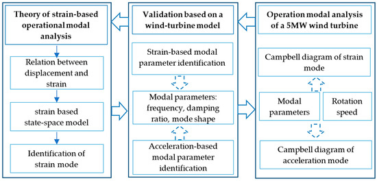
Figure 1.
A flowchart of the paper.
2. Theoretical Background
2.1. Strain-Based Operational Modal Analysis
The dynamic behavior of an elastic vibrating system can be idealized as a differential Equation of vibration, as follows:
where M, C, K are the mass, damping, and stiffness matrices; represents the displacement, velocity, and acceleration vectors at moment t, respectively; and represents the external excitation vector.
The continuous strain responses in the elastic vibrating system can be viewed as the linear superposition of multiple strain modes. The relationship between strain and displacement can be expressed as [19]:
where P is the transformation vector between displacement and strain.
According to Equations (1) and (2), the strain differential Equation of vibration is obtained as:
where Mε, Cε, Kε are satisfied with the following relationship:
The strain state space model is established by constructing the strain state vector and its time rate of change ; the following state space model can then be defined as:
where the ‘con’ is continuous time, represents the strain state matrix, and represents the strain input matrix. These values are given by:
The strain response can be obtained as:
where is the strain observation matrix. can be expressed as:
where is the system observation matrix.
Combining Equations (5) and (8), the strain based continuous-time state-space model is given by:
In the actual measurement process, x(t) and y(t) need to be discretized, and the corresponding state space system Equation can be converted as:
where is the discrete-time state vector; yk is the sampled output vector; and , , and are the discrete state matrix, discrete input matrix, and discrete output matrix, respectively. The classical derivation of discretization can be found in [26]. Considering the effects of noise and system errors in the actual measurement process, the noise Equation is added to the state Equation, and the corresponding state Equation with noise is obtained as follows:
where are the white noise, and the ambient excitation cannot be measured directly in the structural operation state. Therefore, the input term is unknown and is assumed to be white noise. The final strain state space Equation is as follows:
Once the discrete state space Equation of strain is established, and the frequency, damping ratio, and strain modes can be identified by matrices and , the eigen-frequencies , damping ratios , and mode shapes are obtained by:
where Ψ and are the eigenvector and eigenvalue matrices of , with and as discrete and continuous eigenvalues, respectively. represents the sampling period, and denotes the complex modulus.
Modal parameters are identified by eliminating the noise poles from the stabilization diagram. By applying singular value decomposition (SVD) to the formed Toeplitz matrix, the system poles are calculated in a different order. Unstable poles are defined when the poles possess a significantly different identified modal parameter compared to its adjacent order. A stabilization diagram is built by eliminating the unstable poles [17].
2.2. Automated Operational Modal Analysis Algorithm
With the operation of the monitoring system, a massive amount of data are accumulated successively. Therefore, it is important to develop an automated strain-based operational modal analysis algorithm that would help reveal the changing properties of structures under operational conditions.
Automated strain-based operational modal analysis is presented to reveal the variation tendency of structural dynamic parameters without any computer-user interaction. This type of analysis entails the establishment of a stabilization diagram and the selection of stable poles with the assistance of several user-defined parameters [26].
(i) Establishment of the stabilization diagram: The state-space model is estimated using correlation functions with a maximum length of I points. The maximum system order is n, and the stable poles within certain system orders (m, m + j, m + 2j, …, n, where m is the user defined lowest order and j is the increment of order) are considered. Poles are labelled as stable if the relative differences in their natural frequency (), modal damping ratio (), and modal assurance criterion (MAC) values between the poles of consecutive orders are below the following threshold values:
Otherwise, the poles are classified as spurious. At the same time, the poles with unrealistic damping ratios (e.g., ) are discarded.
Figure 2a shows the original stabilization diagram with several spurious poles. These poles will interfere with the automated operational modal analysis. Meanwhile, it is interesting to note that that although the spurious poles are isolated, the stable poles are concentrated around the structural natural frequencies. Thus, the number of spurious poles around a certain frequency is smaller than the number of stable poles representing the structural modes. In order to eliminate these spurious poles, we implement a procedure for the automated selection of stable poles.
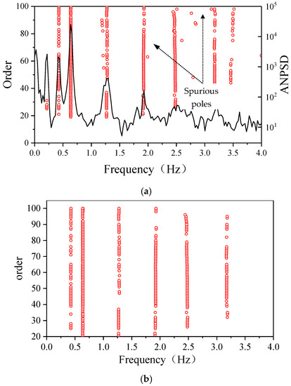
Figure 2.
Original and cleaning stabilization diagrams. (a) Original stabilization diagram; (b) cleaning stabilization diagram.
(ii) Selection of stable poles: (a) In the mth order, different groups are established by examining the modal parameters represented by the poles. (b) In the (m + j)th order, the new poles are incorporated into the corresponding groups if the relative difference of modal parameters is smaller than the threshold prescribed in Step (i). However, if there are any poles in the (m + j)th order that do not match with any groups defined in the previous Step, a new group is assigned. (c) Step (b) is applied to the poles from the (m + 2j)th to the nth order, and all poles are grouped. (d) Subsequently, the number of poles inside each group is counted. It is observed that the stable poles representing structural modes are grouped together, and the corresponding number of poles is relatively large, while the isolated spurious poles are clustered in groups with a small number of poles. (e) Finally, a threshold for the number of poles p is prescribed, and the groups whose numbers of poles are smaller than threshold p are removed. A stabilization diagram obtained after automatically selecting poles is shown in Figure 2b. (f) According to the information represented by the stabilization poles, the modal parameters are estimated by averaging the frequencies, damping ratios, and mode shape vectors within the selected groups of poles.
The parameters of the algorithm, i, j, m, n, and p, used for the automated modal identification in each application, are defined by the user according to the quality of the continuous dynamic monitoring results. In the current application, they are defined as 150, 1, 20, 100, and 10.
3. Strain-Based Operational Modal Analysis of a Scaled Wind Turbine Model
3.1. A Wind Turbine Model and Finite Element Analysis
A vibration test is performed on the wind turbine model to verify the feasibility of the strain-based operational modal analysis algorithm. Figure 3a shows the model in a laboratory; its finite element model is displayed in Figure 3b, and the detailed dimension of the model are listed in Table 1.
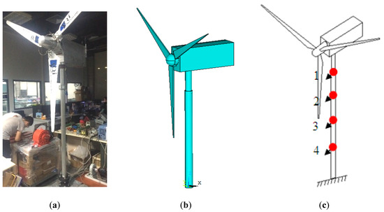
Figure 3.
A wind turbine model, its finite element model, and test setup. (a) The wind turbine model; (b) the finite element model; (c) sensors arranged on the tower.

Table 1.
Size of the wind turbine model in the laboratory (mm).
The numerical simulation is carried out by the ANSYS software as follows: The tower is a cylinder and is modelled by the element solid185. The elastic modulus is 210 Gpa, and the density is 2565 kg/m3. The nacelle is modeled by a solid rectangular mass with Solid185. The elastic modulus is 210 Gpa, and the density is 761 kg/m3. The blade shape is simplified to a triangle, with the end being a short triangular prism. This shape is simulated by the beam3 element, while the stiffness is negligible. The connections between the tower, the nacelle, and the rotor blade are presumed to have infinite stiffness, which is simulated by a constraint Equation. The end of the tower is fixed. The modal analysis is solved by the Block-Lanczos algorithm, and the simulation results will be discussed in Section 3.2.
3.2. Vibration Test of the Wind Turbine Model
Four measurement points (1–4) are arranged on the wind tower, as shown in Figure 3c. At each point, an integrated circuit piezoelectric (ICP) accelerometer and two 120 Ω strain gauges are mounted on the surface of the tower. Two strain gauges form the half bridge of the Wheatstone circuit. One of these gauges records the bending strain of the tower, and the other is for temperature compensation. The acceleration and strain signals are recorded simultaneously by a National Instrument 9234 and cDAQ 9188 data acquisition system. The random excitation of the tower is applied by a rubber hammer. The sampling frequency is 1500 Hz, and then the signal is low filtered and resampled at 300 Hz. The time duration is 200 s.
Figure 4 shows the typical structural responses recorded by both accelerometers and strain gauges. There are several impulse responses captured by the accelerometers, while only two relative deformations are acquired by the strain gauges. It can be inferred that the strain gauges are not sensitive to high frequency components. Meanwhile, Figure 4a shows that the amplitude of strain responses increases gradually from the top to bottom of the tower, while the vibration amplitude of the accelerometers follows a different tendency and decreases slightly, as shown in Figure 4b, in agreement with the long-term vibration behavior observed in the prototype of Areva-M5000 (Figure 9) in Section 4.2.
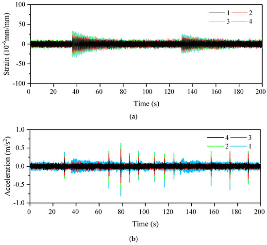
Figure 4.
Structural response of the wind turbine model. (a) Strain responses; (b) acceleration signals.
3.3. Operational Modal Analysis Based on Both Strain and Acceleration Responses
Figure 5 shows the stabilization diagram that was established by applying the automated SSI-COV algorithm to both the strain and acceleration signals. The first two frequencies are identified based on the strain responses (Figure 5a,b) and acceleration signals (Figure 5c,d). Table 2 compares the modal parameters identified by both the strain and acceleration responses, where the modal assurance criterion (MAC) is defined as
where is the modal shape identified by the experiment, and is the numerical simulated results, as shown in Figure 6.
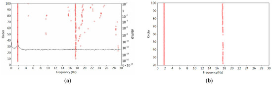

Figure 5.
Identification of the physical modes of the wind turbine model. (a) Strain-based stabilization diagram; (b) cleaning stabilization diagram of (a); (c) acceleration-based stabilization diagram; (d) cleaning stabilization diagram of (c).
Table 2.
Identified modal parameters from the acceleration and strain responses.
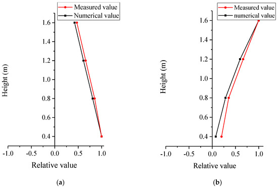
Figure 6.
Comparison of the experimental and simulated mode shapes estimated by both the acceleration and strain responses. (a) First strain-based mode shape; (b) first acceleration-based mode shape.
An inspection of Table 2 shows that the strain- and acceleration-based identification results agree well, although the damping ratios estimated from strain are slightly larger. Moreover, Figure 6 demonstrates that the mode shapes estimated from the acceleration and strain are different. Likely, the strain-based mode shape reflects the distribution of the structural strain instead of vibration deformation, which is characterized by an acceleration-based mode shape. With regard to the first mode shape, Figure 6a shows the fundamental bending mode in which the displacement of the mode grows from the top and reaches its maximum at the foot of the tower. The acceleration-based mode shape in Figure 6b shows an inverse tendency because a relatively larger acceleration response is observed on the top of the tower. These phenomena can be further explained by the main vibrations in both the acceleration and strain responses in Figure 4a,b. Figure 4a reveals that the strain increases gradually from the top to the foot of the tower. Thus, in Figure 4a, the response amplitudes recorded from different strain gauges follow a similar tendency. Oppositely, the acceleration amplitudes in Figure 4b reduce steadily from the top to bottom of the tower because the initial acceleration-based mode shape (Figure 6b) demonstrates that vibration deformation is relatively larger on the top of the tower.
According to above analysis, it may be concluded that strain-based operational analysis methods can efficiently estimate the modal parameters. In the following section, this method will be further implemented to the continuous dynamic data of a 5 MW wind turbine system.
4. Strain-Based Automated Operation Modal Analysis of a 5 MW Wind Turbine
4.1. A Prototype of Areva-M5000
Alpha Ventus is Germany’s first offshore wind farm, consisting of twelve 5 MW wind turbines constructed in the North Sea in 2008. Areva Multibrid M5000 (Figure 7), a full-scale model of a 5 MW wind turbine, was constructed and tested at the Alpha Ventus wind farm. The main technical parameters of the wind turbines are listed in Table 3.
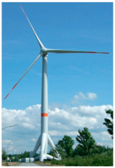
Figure 7.
The Areva-M5000.
Table 3.
Technical parameters of the wind turbine [27].
4.2. A long Term Monitoring System for the Wind Turbine
A long-term monitoring system that supervises all components in the wind turbines system was developed by the Federal Institute for Materials Research and Testing (BAM). This system consists of two independent units mounted at the support and rotor blade to verify the design assumptions, and each unit can record and transfer data individually. The complete monitoring system consists of 111 strain gauges located on five measurement planes, 14 acceleration sensors on six measurement planes, and four inclination sensors on two measurement planes of the support structure [2,27]. In this paper, only two vertical strain gauges installed on the wind tower are used for automated extraction of the modal parameters of the wind turbine. Furthermore, the structural resonance and Sommerfeld phenomenon are analyzed.
The arrangement of both accelerometers and strain gauges are plotted in Figure 8. As shown in Figure 8a,b, the eight accelerometers are mounted on the internal surface of the tower. Y2, Y4, Y6, and Y8 are applied to obtain acceleration along the main wind direction (MWD), while Y1, Y3, Y5, and Y7 are used to measure acceleration in the secondary wind direction (SWD). As plotted in Figure 8c,d, the strain gauges are arranged at section 1Q and 4Q. In section 1Q, three groups of strain rosettes, S1–3, S4–6, and S7–9, are initially designed to estimate the wind load. The vertical strain gauges S2, S5, and S8 are selected to measure the bending strain responses of the wind tower. In the 4Q section, the vertical strain gauge S10 is labeled on the internal surface of the tower in order to test the feasibility of the OMA of a wind turbine system based on the dynamic strain responses.
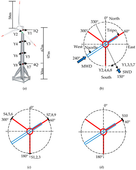
Figure 8.
Arrangement of sensors on the wind turbine: (a) Positions of the eight accelerometers and section 1Q and 4Q; (b) plane view of the wind turbine and wind direction; (c) positions of the strain gauges in section 1Q; (d) positions of the strain gauges in section 4Q.
The signal with a sampling frequency of 50 Hz in two individual units achieved a synchronous result with HBM MGCplus and ran permanently from 1 January 2008 to 31 October 2009. At the beginning of each hour, only the first 8192 points are recorded by all sensors and transferred to the database, thereby forming one setup of data (more than 14,000 setups of data are used). The typical vibration signals acquired by the different sensors under normal operational conditions are shown in Figure 9. Figure 9a shows that the vibration amplitudes of the strain gauge S10 at the bottom of the tower are higher than those on the top S8. Meanwhile, the inverse tendency of the acceleration amplitudes is visible in Figure 9b, where the responses amplitude Y2 on the top of the tower is larger than that at the foot Y8.
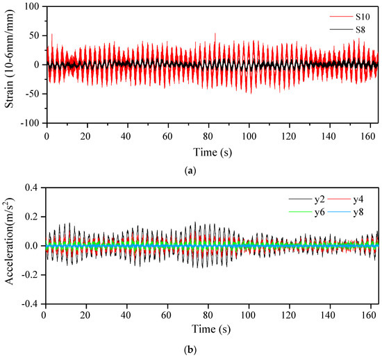
Figure 9.
Typical vibration signals acquired by different sensors with 8192 sampling points: (a) Vibration signals from strain gauges along the main wind direction (MWD); (b) vibration signals from accelerometers along the MWD.
4.3. Strain-Based Automated Operation Modal Analysis of a 5 MW Wind Turbine
The vibration responses from the two strain gauges S8 and S10 along the MWD are processed separately by the automated OMA method introduced in Section 2.2. Figure 1 presents typical plots based on the strain responses. It can be found that the frequencies below 4 Hz can be readily identified. Table 4 lists the averaged modal parameters by both strain and acceleration responses. Meanwhile, according to the finite model analysis in [25], the corresponding calculated frequency is shown to compare it with the identified one. It is noted that the frequency agrees well, while the damping ratios identified by the strain measurements are slightly larger. The mean mode shapes identified by both the accelerometers and strain gauges are plotted in Figure 10. The 1st mode reveals that the deflections on the top of the tower are larger than those at the foot, while the opposite deformation is observed in the mode shape based on the strain measurements. This is similar to the observations in Figure 6. The opposite mode shapes are identified by both the strain and acceleration responses. This phenomenon can also explain the difference in the vibration amplitudes between the acceleration and strain responses shown in Figure 8 and Figure 9.
Table 4.
Averaged values of the modal parameters identified by both the strain sensors and accelerometers.
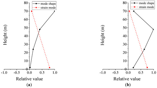
Figure 10.
Mode shape identified by accelerometers y2, y4, y6, and y8 and the strain mode by strain sensors S8 and S10: (a) 1st mode; (b) 2nd mode.
5. Resonance Phenomenon
A significant operational effect resulted from the passage of blades is reported to affect the identified modal parameters of the horizontal wind turbine [1]. In a wind turbine system with three blades, there are two types of resonance induced by different factors, one of which is caused by lateral excitation due to the slightly unbalanced mass of the blades, which leads to periodic vibrations in the tower-nacelle system in the lateral direction, perpendicular to the wind direction. This can be expressed as
where is the lateral excitation frequency of the wind turbine, while f corresponds to the rotation frequency of the blades.
Another type of excitation frequency results from the loading impulse along the wind direction. For the three-blade rotor, the wind turbine system is excited by three times the rotation frequency and its harmonics; that is,
where represents the excitation frequency, and f is the rotation frequency of the blades.
If the above-described excitation frequency meets the structural frequency under operational conditions, structural resonance will occur. This behavior can also be illustrated by the changes in the damping ratio. With regard to the wind turbines in operational states, the total damping ratio is defined as:
where is the structural damping, and is the aerodynamic damping.
The damping of the wind turbine correlates with the nature of the structural material, which reflects the degree of energy loss [28,29]. The interaction between blades and wind leads to a hindrance in the vibration. The aerodynamic load is relative to the relative speed of the blades and wind, so it is named aerodynamic damping. In the operational states, this damping varies according to changes in rotation speed, pitch angle, or wind velocity. When resonance occurs, the aerodynamic damping may become negative and further lead to the variation of the total damping of the wind turbine system. At the same time, the vibration amplitude of the structure will also increase significantly.
To reveal and monitor the resonance phenomenon, the distribution of frequency components is characterized in Figure 11 on the basis of the Averaged Normalized Power Spectral Density (ANPSD) of the strain measurements. Figure 11a plots two ANPSD curves when the wind turbine system is under both operational and non-operational conditions. The former one in red is calculated when the rotation speed is 14.15 rpm, and the latter one in black represents the stage when the rotation speed is 0.07 rpm. Two clear peaks around 1f (14.15/60 = 0.236 Hz) and 3f (3 × 14.15/60 = 0.71 Hz) are noted from the ANPSD when the rotation speed is 14.15 rpm, while only one peak around the fundamental frequency 0.41 Hz is noted from the ANPSD when the rotation speed is only 0.07 rpm, which indicates the existence of the excitation frequency 1f. Figure 11b shows a waterfall plot estimated by sorting the ANPSD for a period of three consecutive days (72 h). Except for the fundamental frequency around 0.41 Hz, peaks in the vicinity of 0.24 Hz and 0.71 Hz are also observed, suggesting that the frequency components are excited by 1f and 3f.
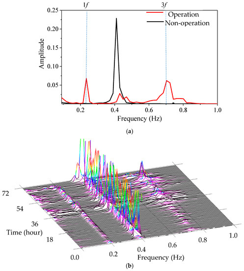
Figure 11.
Frequency distribution of the strain measurements. (a) Averaged normalized power spectral density (ANPSD) produced by the strain responses S8 and S10; (b) waterfall plot based on an ANPSD of S8 and S10.
In order to reveal the adverse 1f and 3nf effects, both the strain and acceleration signals recorded at 50 Hz are low filtered and re-sampled with 5 Hz. Subsequently, the decimated signals are processed by an automated SSI-COV algorithm. The experimental Campbell diagram (Figure 12) can be re-plotted by correlating the identified frequency smaller than 1 Hz and the rotation speed, based on both the strain (S8 and S10) and acceleration (Y2,4,6,8) signals. The analytical frequency Campbell diagram is calculated by Equations (15) and (16), overlapping with the experiential frequencies. The harmonic frequencies 1f, 3f, 6f, and 9f are clearly observed with an increase in rotation speed. Under operational conditions over nearly two years, we found that the identified frequencies of 1f do not meet the structural fundamental frequency around 0.41 Hz due to the mass imbalance of the blades.
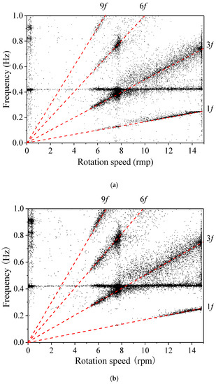
Figure 12.
Analytical and experimental frequency Campbell diagram based on low filtered and re-sampled strain and acceleration responses. (a) Eigen frequencies estimated by the dynamic strain responses acquired from S8 and S10; (b) Eigen frequencies estimated by the acceleration responses acquired from y2,4,6,8.
The damping ratio is an important design parameter for wind turbines because it influences structural fatigue analysis and expected lifetime. As described in Equation (17), the identified damping value is composed of structural damping and aerodynamic damping. The former is approximately assumed to be a constant, while the latter varies with an aeroelastic interaction of the wind flow and the wind turbine. As shown in Figure 13, the classical Campbell diagram is extended to describe the variation tendency of the damping ratio depending on the rotational speed of the wind blades. The corresponding damping ratios of these frequencies estimated from both the strain and acceleration signals from 0.40 Hz to 0.45 Hz are selected. Figure 13 shows the correlation of rotation speed and the mean/median values with a gap of 0.5 rpm. Similar variation tendencies between the mean/median damping ratio and the rotation speed are observed in Figure 13a,b. When the rotation speed stays below 0.5 rpm, the wind turbine system is non-operational because the rotation speed remains at a low level. The mean/median values of the damping ratios estimated from both the strain and acceleration signals are 0.77%/0.50% and 0.56%/0.35%, respectively. These values only reflect the structural material damping. When the blades start rotating at a speed from 5.5 to 6.0 rpm, the corresponding damping ratio values jump to 1.69%/1.21% (strain) and 1.91%/1.02% (acceleration). As the rotation speed approaches 8 rpm, all the damping ratios first rise and then decrease to 0.82%/0.51% and 0.91%/0.46%. Afterwards, the damping ratio values retain an upward tendency, with the rotation speed increasing to 12.5 rpm. Subsequently, all the damping ratios reduce slightly again.
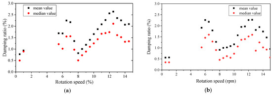
Figure 13.
Campbell diagram for the damping ratio. (a) Averaged damping ratios identified from the strain measurements within an interval of 0.5 rpm; (b) averaged damping ratios identified from the acceleration measurements within an interval of 0.5 rpm.
Figure 13 plots the vibration amplitude of the wind turbine, evaluated by the strain or acceleration responses, against the rotation speed. The root mean square (RMS) of both strain gauges S10 and S8 as well as accelerometers Y2 and Y8 are calculated on the basis of the vibration signals for 8192 points each hour. Over nearly two years, the mean value of all RMSs is calculated as the Rmean. The vibration amplitude of the wind tower is evaluated by the ratio RMS/Rmean. Figure 14 shows that a similar trend of the vibration amplitude depends on the rotation speed. In Figure 14a,b, the strain-based vibration amplitude rises slightly when the blades start rotating at 5.5 rpm. When the rotation speed of the blades approaches 7.5–8 rpm, the amplitude rises quickly and then reaches its peak value. Subsequently, the vibration amplitude decreases slowly as the rotation speed varies from 8 to 10 rpm. A similar variation tendency is also observed for the acceleration-based vibration amplitude in Figure 14c,d. The difference is that a relatively large strain amplitude is observed at the foot of the tower (Figure 14b), while a correspondingly larger acceleration amplitude is found at the top of the tower (Figure 14d).
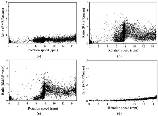
Figure 14.
Vibration amplitude evaluated by the ratio RMS/Rmean versus the rotation speed. (a) The ratio RMS/Rmean calculated by strain gauge S8 at the top of the tower; (b) the ratio RMS/Rmean calculated by strain gauge S10 at the foot of the tower; (c) the ratio RMS/Rmean calculated by accelerometer Y2 at the top of the tower; (d) the ratio RMS/Rmean calculated by accelerometer Y8 at the foot of the tower.
The resonance phenomenon is clearly observable according to the Campbell diagram for the frequency, damping ratio, and vibration amplitude based on both the strain and acceleration responses. In Figure 12, when the rotation speed reaches around 8.0 rpm, 3f represents the frequency of the blades’ passage, which approaches 3f = 3 × 8.0/60 = 0.40 Hz, crossing the identified first frequency of the structure (0.41 Hz). As seen in Figure 13, the estimated damping ratio varies with the rotation speed of the blades and reaches its minimum value near 8 rpm, where 3f matches the first frequency. The resonance of the wind turbine can be further verified by the vibration amplitude in Figure 14. When the blade rotation speed reaches near 8 rpm, both the strain and acceleration amplitude rise rapidly and became even larger than the values observed with the blade under its maximum rotation speed of 14.8 rpm. Figure 11, Figure 12 and Figure 13 demonstrate that the wind tower responses recorded by only two strain gauges and processed by the automated OMA algorithm can capture the resonance phenomena of a wind turbine in an operational state.
The long-term performance of the wind turbine in Figure 14 and Figure 15 may be partially explained by the Sommerfeld effect. In 1902, Arnold Sommerfeld first observed this problem in a vibration system consisting of an unbalanced motor and its elastic foundation [30,31,32]. In 2004, R.M.L.R.F. Brasil attempted to theoretically prove the existence of the Sommerfeld Effect in a wind turbine supporting tower [33]. Sommerfeld’s observation showed that the structural response of the system may act like an energy sink under certain conditions so that a part of the external energy is spent to vibrate the structure rather than to increase the rotation speed. Usually, the Sommerfeld effect concerns the dynamics of a system composed of an unbalanced electric motor placed on a flexible support. In this system, the gradually increasing energy supply increases the rotational speed of the motor until it approaches the structure’s fundamental frequency. As the energy supply is increased further, the motor speed remains the same until it suddenly jumps to a much higher value (simultaneously, the amplitude drops to a much lower value) upon exceeding a critical power input limit. Similar phenomena were also observed when the power was gradually reduced.
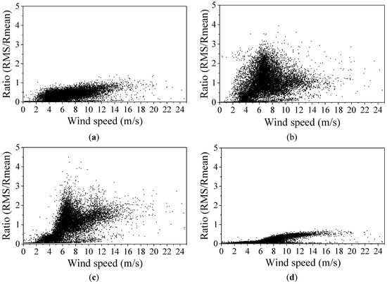
Figure 15.
The ratio RMS/Rmean calculated by the strain and acceleration responses against the wind velocity. (a) The ratio RMS/Rmean calculated by the strain gauge S8 at the top of the tower; (b) the ratio RMS/Rmean calculated by the strain gauge S10 at the foot of the tower; (c) the ratio RMS/Rmean calculated by accelerometer Y2 at the top of the tower; (d) the ratio RMS/Rmean calculated by accelerometer Y8 at the foot of the tower.
In a horizontal wind turbine system, the wind blades act as the motor, while the wind tower serves as the flexible support. These components form a non-ideal vibration system under external wind energy. In Figure 14b,c, when the corresponding blade passage frequency of 0.40 Hz (8 rpm) is close to the fundamental frequency of 0.41 Hz (Figure 11), the structural vibration amplitude of both the strain and acceleration responses increases rapidly, indicating that the structure is jammed by its resonance and the Sommerfeld effect. At this stage, the additional energy harvested from wind induces an increase in the vibration amplitude instead of improving the rotation speed. This phenomenon is evidenced by the dynamic amplitude evaluated by both the acceleration and strain responses in Figure 15. It can be found the strain amplitudes of S10 and S8 increase with an increase in wind velocity (Figure 15a,b). A similar phenomenon is also noted in the acceleration amplitude plotted in Figure 15c,d. The difference is that the relatively large strain amplitude is observed at the foot of the tower, while the correspondingly high acceleration amplitude is located at the top of the tower and is caused by the difference between the strain and acceleration modes’ shapes.
6. Conclusions
This paper presents a strain-based automated modal identification method and its application to a 5 MW horizontal wind turbine system to monitor the adverse resonance phenomenon under operational conditions. The strain-based method is validated by comparing it with the acceleration-based approach.
Firstly, the feasibility of the strain-based automated modal identification algorithm is validated by a scaled wind turbine model. Compared with the acceleration-based method, similar frequency and modal damping results are observed, but the mode shape is completely opposite. Thus, the strain-based mode shape reflects the distribution of stress instead of vibration deformation, which is characterized by an acceleration-based mode shape. Subsequently, the proposed method is applied to the strain responses acquired from the wind tower over two years. The modal parameters are estimated automatically and are compared with those extracted from the acceleration responses. Both the strain and acceleration response can be used to track the variations in the 1f, 3f excitation frequency and fundamental frequency in the Campbell diagram. A significant structural resonance phenomenon is found because due to the coincidence of the excitation frequency 3f and the fundamental frequency of the wind turbine. As the blade rotation speed is close to 8 rpm, the damping ratio decreases, and the strain increases. With an increase in wind velocity, the rotation speed is limited to around 8 rpm, and the extra energy is wasted to increase the structural vibration amplitude. The wind turbine system is always locked in a resonance state.
The proposed strain-based automated modal identification algorithm, with only two strain gauges mounted on the wind tower, can efficiently monitor this adverse phenomenon by tracking the variation of 1f, 3f and the fundamental frequencies of the horizontal wind turbine system in an operational state.
A horizontal wind turbine is a time-varying system under operational conditions. In the future, the strain-based time-varying operational modal analysis algorithm will be further developed to more accurately track modal properties.
Author Contributions
Conceptualization, R.G.R. and S.S.; methodology, W.-H.H.; M.W.; D.-H.T.; writing—original draft preparation, M.W., D.-H.T., J.-L.L.; writing—review and editing, W.-H.H., Z.-H.L., W.L.; supervision, J.T. All authors have read and agreed to the published version of the manuscript.
Funding
This research was funded by the National Natural Science Foundation of China: No. 51878226 and No. 51678201. It is also funded by the Guangdong Provincial Natural Science Foundation: 2017A030313292 and the Fundamental Research Funds for the Central Universities.
Acknowledgments
The first four authors gratefully acknowledge the support by the National Natural Science Foundation of China: No. 51878226 and No. 51678201. The first three authors also acknowledge the support from the Guangdong Provincial Natural Science Foundation: 2017A030313292. The first author acknowledges the support from the Fundamental Research Funds for the Central Universities. All authors are grateful to the department of Safety Structures at the Federal Institute for Materials Research and Testing (BAM VII.2) for providing the measurement data.
Conflicts of Interest
The authors declare no conflicts of interest.
References
- Gasch, R.; Twele, J. Wind power plants: Fundamentals, Design, Construction and Operation, 2nd ed.; Springer: Berlin/Heidelberg, Germany, 2012. [Google Scholar]
- Rohrmann, G.R.; Thöns, S.; Rücker, W. Integrated Monitoring of Offshore Wind Turbines -Requirements, Concepts and Experiences. Struct. Infrastruct. Eng. 2010, 6, 575–591. [Google Scholar] [CrossRef]
- Márquez, F.; Tobias, A.; Pérez, J.; Papaelias, M. Condition monitoring of wind turbines: Techniques and methods. Renew. Energy 2012, 46, 169–178. [Google Scholar] [CrossRef]
- Wymore, M.; Van Dam, J.; Ceylan, H.; Qiao, D. A survey of health monitoring systems for wind turbines. Renew. Sustain. Energy Rev. 2015, 52, 976–990. [Google Scholar] [CrossRef]
- Adams, D.; White, J.; Rumsey, M.; Farrar, C.R. Structural health monitoring of wind turbines: Methods and application to a HAWT. Wind Energy 2011, 14, 603–623. [Google Scholar] [CrossRef]
- Cunha, A. Special Section: Reviews on Structural Dynamics Applications in Civil Engineering, Preface. J. Sound Vib. 2015, 334, 1. [Google Scholar] [CrossRef]
- Brincker, R.; Ventura, C. Introduction to Operational Modal Analysis; John Wiley & Sons Ltd.: Chichester, UK, 2015. [Google Scholar]
- Chauhan, S.; Tcherniak, D.; Basurko, J.; Salgado, O.; Urresti, I.; Carcangiu, C.E.; Rossetti, M. Operational modal analysis of operating wind turbines: Application to measured Data. In Rotating Machinery, Structural Health Monitoring, Shock and Vibration; Springer: New York, NY, USA, 2011; Volume 5, pp. 65–81. [Google Scholar]
- Ozbek, M.; Rixen, J.D. Operational modal analysis of a 2.5 MW wind turbine using optical measurement techniques and strain gauges. Wind Energy 2013, 16, 367–381. [Google Scholar] [CrossRef]
- Zierath, J.; Rachholz, R.; Rosenow, S.E.; Bockhahn, R.; Schulze, A.; Woernle, C. Experimental identification of modal parameters of an industrial 2 MW wind turbine. Wind Energy 2018, 21, 338–356. [Google Scholar] [CrossRef]
- Dai, K.; Wang, Y.; Huang, Y.; Zhu, W.; Xu, Y. Development of a modified stochastic subspace identification method for rapid structural assessment of in-service utility-scale wind turbine towers. Wind Energy 2017, 20, 1687–1710. [Google Scholar] [CrossRef]
- Devriendt, C.; Magalhães, F.; Weijtjens, W.; De Sitter, G.; Cunha, Á.; Guillaume, P. Structural health monitoring of offshore wind turbines using automated operational modal analysis. Struct. Health Monit. 2014, 13, 644–659. [Google Scholar] [CrossRef]
- Hu, W.-H.; Thöns, S.; Rohrmann, R.G.; Said, S.; Rücker, W. Vibration-based structural health monitoring of a wind turbine system. Part I: Resonance phenomenon. Eng. Struct. 2015, 89, 260–272. [Google Scholar] [CrossRef]
- Oliveira, G.; Magalhães, F.; Cunha, A.; Caetano, E. Continuous dynamic monitoring of an onshore wind turbine. Eng. Struct. 2018, 164, 22–39. [Google Scholar] [CrossRef]
- Dong, X.; Lian, J.; Wang, H.; Yu, T.; Zhao, Y. Structural vibration monitoring and operational modal analysis of offshore wind turbine structure. Ocean. Eng. 2018, 150, 280–297. [Google Scholar] [CrossRef]
- Zhao, Y.; Pan, J.; Huang, Z.; Miao, Y.; Jiang, J.; Wang, Z. Analysis of vibration monitoring data of an onshore wind turbine under different operational conditions. Eng. Struct. 2020, 205, 110071. [Google Scholar] [CrossRef]
- Lennart Ljung: System Identification-Theory for the User, 2nd ed.; PTR Prentice Hall: Upper Saddle River, NJ, USA, 1999.
- Bart, P.; Auweraer, H.V.D.; Guillaume, P.; Leuridan, J. The PolyMAX frequency-domain method: A new standard for modal parameter estimation? Shock Vib. 2004, 11, 395–409. [Google Scholar]
- Yam, L.Y.; Leung, T.P.; Li, D.B.; Xue, K.Z. Theoretical and experimental study of modal strain analysis. J. Sound Vib. 1996, 191, 251–260. [Google Scholar] [CrossRef]
- Santos, F.L.M.D.; Peeters, B.; Lau, J.; Desmet, W. An overview of experimental strain-based modal analysis methods. In Proceedings of the 26th International Conference on Noise and Vibration Engineering, Leuven, Belgium, 15–17 September 2014. [Google Scholar]
- Cheng, L.; Busca, G.; Cigada, A. Experimental strain modal analysis for beam-like structure by using distributed fiber optics and its damage detection. Meas. Sci. Technol. 2017, 28, 074001. [Google Scholar] [CrossRef]
- Wang, T.; Celik, O.; Catbas, F.N. A frequency and spatial domain decomposition method for operational strain modal analysis and its application. Eng. Struct. 2016, 114, 104–112. [Google Scholar] [CrossRef]
- Santos, F.L.M.D.; Peeters, B.; Desmet, W.; Goes, L.C.S. Strain-based experimental modal analysis on planar structures: Concepts and practical aspects. Top. Modal Anal. Test. 2016, 10, 335–346. [Google Scholar]
- Presas, A.; Luo, Y.; Wang, Z.; Guo, B. Fatigue life estimation of Francis turbines based on experimental strain measurements: Review of the actual data and future trends. Renew. Sustain. Energy Rev. 2019, 102, 96–110. [Google Scholar] [CrossRef]
- Thöns, S.; Faber, M.H.; Rücker, W. Fatigue and serviceability limit state modelbasis for assessment of offshore wind energy converters. ASME J. Offshore Mech. Arct. Eng. 2012, 134, 031905. [Google Scholar] [CrossRef]
- Hu, W.-H.; Caetano, E.; Cunha, A. Structural health monitoring of a stress-ribbon footbridge. Eng. Struct. 2013, 57, 578–593. [Google Scholar] [CrossRef]
- Rücker, W.; Fritzen, C.P.; Rohrmann, R.G. IMO-WIND Integrated system for monitoring and assessment of offshore wind turbines. In BAM-University of Siegen Joint Report on the Projects Innonet 16INO326 and 16INO327; BAM: Berlin, Germany, 2010. [Google Scholar]
- Salzmann, D.J.C.; Van der Tempel, J. Aerodynamic damping in the design of support structures for offshore wind turbines. In Copenhagen Offshore Wind Conference; European Offshore Wind Conference & Exhibition: Copenhagen, Denmark, 2005. [Google Scholar]
- Liu, X.; Lu, C.; Liang, S.; Godbole, A.; Chen, Y. Vibration-induced aerodynamic loads on large horizontal axis wind turbine blades. Appl. Energy 2017, 185, 1109–1119. [Google Scholar] [CrossRef]
- Sommerfeld, A. Beitraege zum dynamischen ausbau der festigkeitslehre. Physikal Zeitschr 1902, 3, 266–286. [Google Scholar]
- Eckert, M. The Sommerfeld effect: Theory and history of a remarkable resonance phenomenon. Eur. J. Phys. 1996, 17, 285–289. [Google Scholar] [CrossRef]
- Cveticanin, L.; Zukovic, M.; Balthazar, J.M. Dynamics of Mechanical Systems with Non-Ideal Excitation; Springer: Berlin/Heidelberg, Germany, 2018. [Google Scholar]
- Samantaray, A.K. Steady-state dynamics of a non-ideal rotor with internal damping and gyroscopic effects. Nonlinear Dyn. 2009, 56, 443–451. [Google Scholar] [CrossRef]


© 2020 by the authors. Licensee MDPI, Basel, Switzerland. This article is an open access article distributed under the terms and conditions of the Creative Commons Attribution (CC BY) license (http://creativecommons.org/licenses/by/4.0/).