Article

Stochastic 3D Carbon Cloth GDL Reconstruction and Transport Prediction

School of Automotive Studies, Tongji University, Shanghai 200000, China
*
Author to whom correspondence should be addressed.
Energies 2020, 13(3), 572; https://doi.org/10.3390/en13030572
Submission received: 26 December 2019 / Revised: 14 January 2020 / Accepted: 22 January 2020 / Published: 24 January 2020
(This article belongs to the Special Issue Latest Progress for Proton Exchange Membrane Fuel Cells)

Abstract

:
This paper presents the 3D carbon cloth gas diffusion layer (GDL) to predict transport behaviors of anisotropic structure properties. A statistical characterization and stochastic reconstruction method is established to construct the 3D micro-structure using the data from the true materials. Statistics of the many microstructure characteristics, such as porosity, pore size distribution, and shape of the void, are all quantified by image-based characterization. Furthermore, the stochastic reconstruction algorithm is proposed to generate random and anisotropic 3D microstructure models. The proposed method is demonstrated by some classical simulation prediction and to give the evaluation of the transport properties. Various reconstructed GDLs are also generated to demonstrate the capability of the proposed method. In the end, the adapted structure properties are offered to optimize the carbon cloth GDLs.

1. Introduction

Among different types of fuel cells, the proton exchange membrane fuel cell (PEMFC) has become one of the most promising clean energy technologies in the 21st century. PEMFC directly converts the chemical energy stored in the hydrogen fuel into electrical energy, with water being the only by-product [1]. Due to its long working life, strong temperature adaptability, fast starting speed, simple operation, and convenient installation, PEMFC can be widely used in important fields such as transportation, military, aerospace and communication.
As a vital part in PEMFC, the gas diffusion layer (GDL) serves as a support in membrane-electrode assembly (MEA) and plays a central role in mass transport [2]. GDL is a porous layer composed of randomly oriented carbon fibers that are either woven (carbon cloth) or no-woven (carbon paper). Carbon paper shapes like cardboard and carbon cloth is similar to the style of woven fabric [3].
The GDL has a complex pore structure and its transmission characteristics have an important influence on the performance of PEMFC. Many scholars have conducted researches on their effects through experiments and numerical methods [4,5,6]. Most of the experiments only focused on the surface characteristics of GDL and are time- and effort-consuming. Thus, researchers recently have adopted more numerical simulation methods which are more easily implemented. The GDL models used for numerical simulation mainly include macroscopic models [7,8] and microscopic pore-scale models [9,10]. The former ignores the structural influence of microscopic pores inside the material and assumes GDL as a homogeneous material. The latter uses 3D reconstruction technology to construct the microstructure of GDL, and then studies its transmission characteristics by means of mesoscopic or microscopic numerical analysis [11]. Since the GDL is made of porous materials which have a complex pore structure, how to construct a model more conforming to the real GDL has become a hotspot in recent years. Commercial packages are also available for generating both woven carbon cloth and non-woven carbon paper GDL.
At present, to perform GDL microstructure reconstruction, there are two common methods, namely groups of images combination technique [12] and stochastic technique [5,13]. In the former technique, sequential images of a GDL are provided by X-ray tomography and then, these images are integrated to reconstruct the 3D GDL micros-model. In the latter method, a stochastically generated 3D virtual model is conformed to the microstructure by adapting the geometric model parameters. In 2016, Shojaeefard et al. [11] published a review on the research progress of PEMFC porous electrode microstructure reconstruction, which introduces in detail the research process, methods and results of 3D reconstruction GDL by these two techniques. Koido et al. [14] first obtained the carbon paper GDL (Sample: Toray TGP-H-060) structure by X-Ray CT technique in 2008, then they used the thinning algorithm of image processing technology to obtain the number of connected pores. This method was later used in several papers on carbon paper GDL published by Ostadi [15,16], Rama [17,18] and Garcia Salaberri et al. [19,20]. The widely used GDL stochastic reconstruction technique is the simple model of carbon paper GDL with the least possible parameters proposed by Schaladitz et al. [21] in 2006. D Froning et al. [22,23] established a stochastic reconstruction model of carbon paper GDL based on the real structure, simulated the gas transport in the microstructure of carbon paper GDL, and analyzed the impact of compression on the transmission process. Compared with the reconstruction of carbon paper GDL, the actual carbon cloth GDL has a more complex structure and larger curvature, and requires more input of structural parameters in the reconstruction progress. Therefore, the stochastic reconstruction of carbon cloth GDL is more difficult. However, the carbon cloth GDL has a relatively regular geometry and low randomness, so a simplified stochastic model makes it easier to determine the input parameters [11].
In this paper, based on Salomov’s carbon cloth GDL stochastic reconstruction method, we propose a new reconstruction method to generate a carbon cloth GDL model. The structure obtained by this new stochastic method displays more realistic visual effect and more accurate characterization of GDL samples. Then, we adjust the structural parameters of the reconstructed model. Several different porosities and fiber radii are chosen to reconstruct carbon cloth models. Finally, taking tortuosity and permeability as examples, in this paper we studied how the value of tortuosity and permeability of different carbon cloth models change with different porosity and fiber radius.

2. Methodology

2.1. The Microstructure Reconstruction Model of Carbon Cloth GDL
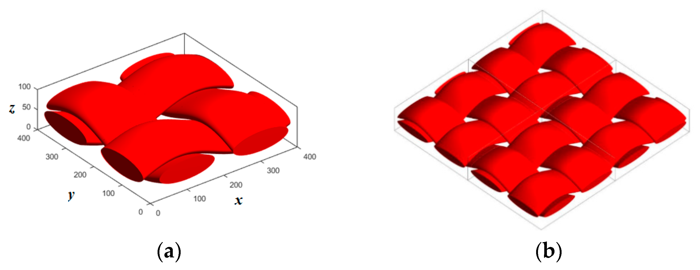
Based on the published papers, carbon cloth is woven from multiple bundles and each bundle is composed of multiple carbon fibers. Until recently, there are few works on stochastically reconstruction of carbon cloth GDL. The only paper reported by Salomov et.al [24] provides an example on how to get a characteristic cell consists of four orthogonal bundles of carbon fibers. In their model, they considered the x-direction as the main flow direction and the yz-direction as a woven plane. The main assumptions are as follows:
(i)
Carbon cloth fibers are divided into two pairs of mutually orthogonal bundles.
(ii)
Each bundle has an elliptic cross-section.
(iii)
A bundle consists of many fibers, which distributed homogeneously.
(iv)
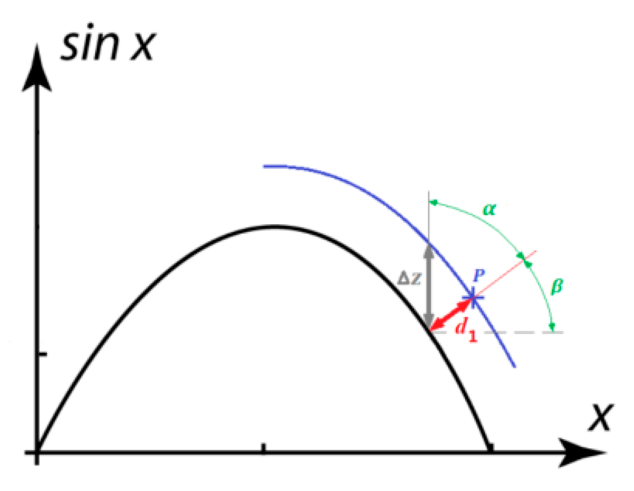
A fiber is considered as a cylinder with a sinusoidal directrix.
The basic parameters they needed are the fiber radius r and the average distance d between two nearest neighbor fibers within a bundle, which were obtained by SEM images of carbon cloth and after complex geometric relations calculation. Owing to the regularity of fibers, the two parameters are adequate for reconstructing the carbon cloth. The reconstruction process is as follows:
(i)
Generating an elliptic bundle of cylinder fibers with a given radius.
(ii)
Merging two elliptic bundles into a 2D slice.
(iii)
Generating of all 2D slices by changing the centers of fiber sections along the sinusoidal directrix. There were two directrixes inside each slice and one was shifted relative to the other by half the wavelength.
(iv)
Creating the orthogonal fibers in a similar way and then assembly of the two pairs of fibers.
The assumptions of their method means the structure cannot truly reflect the complex pore structure characterization inside the GDL, but the reconstruction process is different. Based on the above assumptions and using the powerful array arithmetic function of MATLAB, we propose two carbon cloth reconstruction models. One is the bunched fiber model, which consists of regular fiber bundles with an elliptic cross-section and each fiber bundle is regarded as a whole. The other is the single fiber model, which consists of several single fibers randomly distributing in an elliptic cross-section to form a fiber bundle. This model is more visually similar to the real carbon cloth.

2.2. The Bunched Fiber Model of Carbon Cloth GDL

Carbon cloth GDLs are modeled using deterministic methods because of its woven cyclic pattern. Thus, a primitive cell (see in Figure 1) is complete to represent the minimum geometric information of reconstruction instead of generating the whole sample. These primitive cells can be attached unlimited times to form a bigger carbon cloth GDL at the required dimensions. Therefore, it is possible to overlap several layers to form a thicker sample.
The primitive cell consists of four woven compact bundle of fibers with a constant elliptic section as shown in Figure 1. These bundles run along a sinusoidal guiding curve that passes through the center of the bundle. The sinusoidal guiding curve can be defined in a Cartesian coordinate system:
z = A sin ( 2 π x L ) y = c o n s t
where A is the amplitude of the sinusoidal curve and L is wavelength. The given equations can only get two of the four bundles of the primitive cell at x-direction. However, the other two bundles have a similar form with swap of x and y variables along y-direction.
In order to convert the difference between the ordinates of two points on the same abscissa of two curves into the vertical distance between the two curves, we introduce a correction coefficient ε (see in Figure 2, ∆z is the difference between the ordinates and d1 is the vertical distance between two curves):
d 1 = Δ z cos α = Δ z sin β = Δ z 1 + ( 2 π A L ) 2 cos 2 ( 2 π L x ) = ε Δ z
Namely, the correction coefficient ε is:
ε = 1 1 + ( 2 π A L ) 2 cos 2 ( 2 π L x )
From the previous results and given the elliptic of the fiber cross-section, an arbitrary point P(x, y, z) should meet the following condition to be contained by the fiber:
( ε z A sin ( 2 π x / L ) R v ) 2 + ( y c o n s t R h ) 2 1
where Rv and Rh are the semi-minor and semi-major axis of an elliptical cross-section, respectively. The above condition is true for fibers in the x-direction. For the fibers in the y-direction, the condition needs to swap the variables x and y:
( ε z A sin ( 2 π y / L ) R v ) 2 + ( x c o n s t R h ) 2 1
The bunched fiber model is designed for input parameters: the minor and major radius of elliptic cross-section, the amplitude of the guiding curve and its wavelength. Through multiple simulations, it is found that the wavelength can be taken to be 4.5 times the major radius. The carbon cloth model reconstructed under this condition can completely present the pores between the fiber bundles. The generated microstructure of the primitive cell can be stored in a 3D binary array. If a voxel belongs to the fibers according to the two conditions above, the value of array element corresponding the voxel will be set to one. If not, then the value of array element will be set to zero. Therefore, all number 1 represents fibers and number 0 means pores in the 3D binary array. This binary array is called the 3D digital model of carbon cloth.

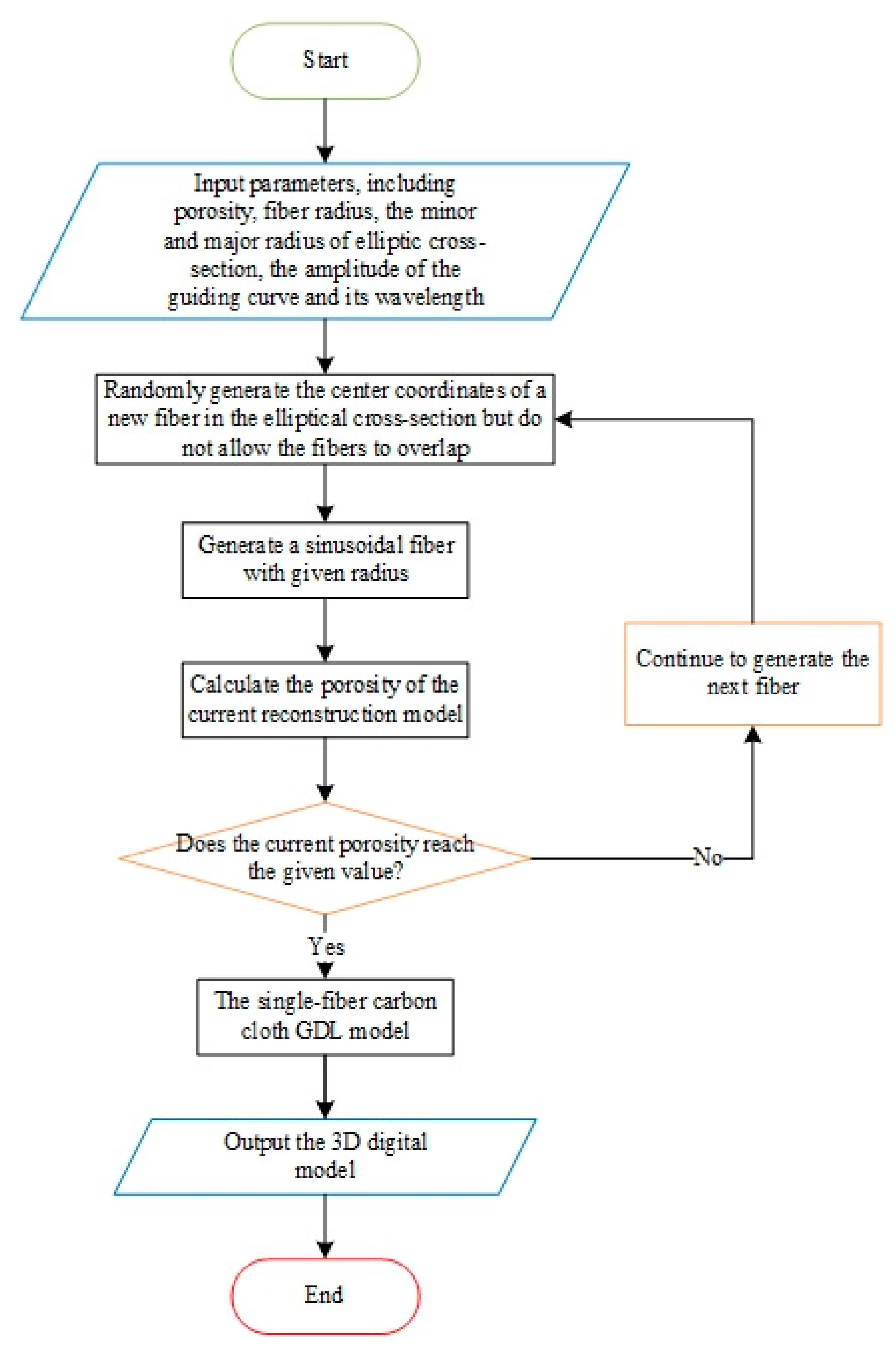
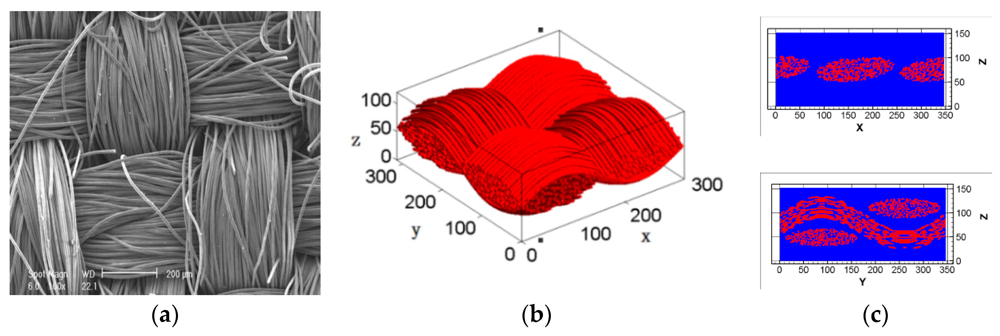
2.3. The Single Fiber Model of Carbon Cloth GDL

Based on the bunched fiber model, the single fiber model is given to obtain a more precise digital sample of carbon cloth GDL with more adjustable parameters. Four bundles are formed by many single cylinder fibers respectively. The conditions met by an arbitrary point P(x, y, z) are changed into the following forms for x,y directions:
( z z i A sin ( 2 π x / L ) r ) 2 + ( y y i c o n s t r ) 2 1 ( z z i A sin ( 2 π x / L ) r ) 2 + ( x x i c o n s t r ) 2 1
where (yi/xi, zi) is the coordinate of the ith cylinder fiber center in the elliptical bundle, r is the fiber radius and A is the amplitude of the sinusoidal curve mentioned in Section 2.2. The coordinates of the fiber centers are randomly generated in the elliptical bundle. When the semi-minor and semi-major axis of elliptical bundle, the radius of carbon fiber and the porosity of the carbon cloth are all given, the number of fibers can be calculated. The detailed reconstruction process is shown in Figure 3.
Figure 4 shows the single fiber carbon cloth GDL model generated by MATLAB. Compared with the bunched fiber model of carbon cloth GDL, the single fiber model is more virtually similar to the real carbon cloth. The stochastic distribution of fibers makes the carbon cloth exhibit anisotropic characteristics in three directions, rather than the homogeneous structure constructed by previous researchers. It expresses more complex characteristics inside the structure and has more adjustable parameters. The structure parameters are embedded in the model, so that the structural samples can better reflect the complex pores in the carbon cloth, realize multi-structure adjustability, and provide support for seeking optimal structural parameters.
The relationship of porosity between the two samples is defined as:
p s = 1 e ( 1 p b )
where ps and pb are the porosity of the single fiber and the bunched fiber sample of carbon cloth GDL respectively. The porosity is the ratio of the number of all zeros and all elements for 3D binary array, e is the area proportion of all circles and ellipse. The generating time of bunched fiber is obviously much less than the single fiber model, so Equation (7) can be used to calculate ps quickly to study the effect of structural parameters on porosity of carbon cloth GDL.

2.4. Determination of the Anisotropic Permeability and Tortuosity

Permeability and tortuosity are key parameters that characterize the pore structure and the transmission properties of porous materials. The permeability is used to represent the anisotropic properties of a porous material. Permeability of a porous media describes how easily a fluid can pass through its porous structure when subjected to a given pressure drop. The tortuosity is a characteristic parameter of the degree of bending of the interconnected pores in the reacting porous medium.

2.4.1. Calculation of Permeability

The permeability tensor is usually used to represent the anisotropic properties of a porous medium. Permeability represents the ability of a fluid passing through a given porous medium. The mechanics of the flow is governed by the Navier–Stokes equation:
d d t ( ρ u ) + ( ρ u u ) = P + η 2 u
where ρ is the density of the fluid, u is the velocity, ∇P is the pressure gradient, and η is the dynamic viscosity of the fluid. When the fluid flow reaches steady state, the permeability of the medium can be calculated based on Darcy’s law:
q = K P η
where q is the volumetric average for fluid flux and K is the permeability.
When a fluid in a porous medium is subjected to a pressure gradient in z-direction, it will not only flow in the direction in which the pressure is applied, but also flow in the x- and y-directions due to the connectivity between the pores. Therefore, 9 permeability components can be obtained depending on the direction of pressure application.
When applying the pressure drop in the x-direction:
K x x = ρ μ q x ( P / L x ) ; K x y = ρ μ q y ( P / L x ) ; K x z = ρ μ q z ( P / L x )
When applying the pressure drop in the y-direction:
K y x = ρ μ q x ( P / L y ) ; K y y = ρ μ q y ( P / L y ) ; K y z = ρ μ q z ( P / L y )
When applying the pressure drop in the z-direction
K z x = ρ μ q x ( P / L z ) ; K z y = ρ μ q y ( P / L z ) ; K z z = ρ μ q z ( P / L z )
where Lx/y/z is the length of digital model in the x-, y- and z-direction, respectively, qx, qy, qz are the average flow rates and are calculated by:
q x = c 3 i u i , x L x L y L z ; q y = c 3 i u i , y L x L y L z ; q z = c 3 i u i , z L x L y L z
where c is the acoustic speed, ui,x, ui,y, ui,z are the fluid velocity components at the ith lattice in the x-, y- and z-directions, respectively.

2.4.2. Calculation of Tortuosity

For a porous medium, the tortuosity quantifies the microscopic flow deviation and the degree of curvature of pores inside the medium. The tortuosity λ is defined as the ratio of the free diffusion coefficient of a gas in free space D0 to its effective diffusion coefficient in the porous medium De:
λ = D 0 D e
The free diffusion coefficient for a gas can be calculated by:
D 0 = δ x 2 ( τ 0.5 ) / 3.5 δ t
where τ is the relaxation time parameter. The diffusion of a gas in the porous medium is simulated by applying a concentration difference at both ends of the structural model in the same direction. Assuming that the concentration difference is applied in the z-direction, the effective diffusion coefficient in this direction can be calculated by:
D e = L N Δ c i = 1 N q z , i
where N is the total number of pore voxels in our 3D digital model, Δc is the concentration difference, and L is the length of our model along the direction which the concentrate differs.

3. Results and Discussion

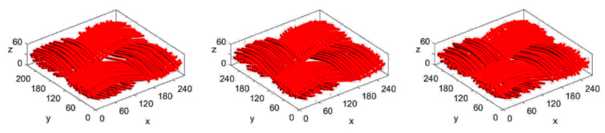
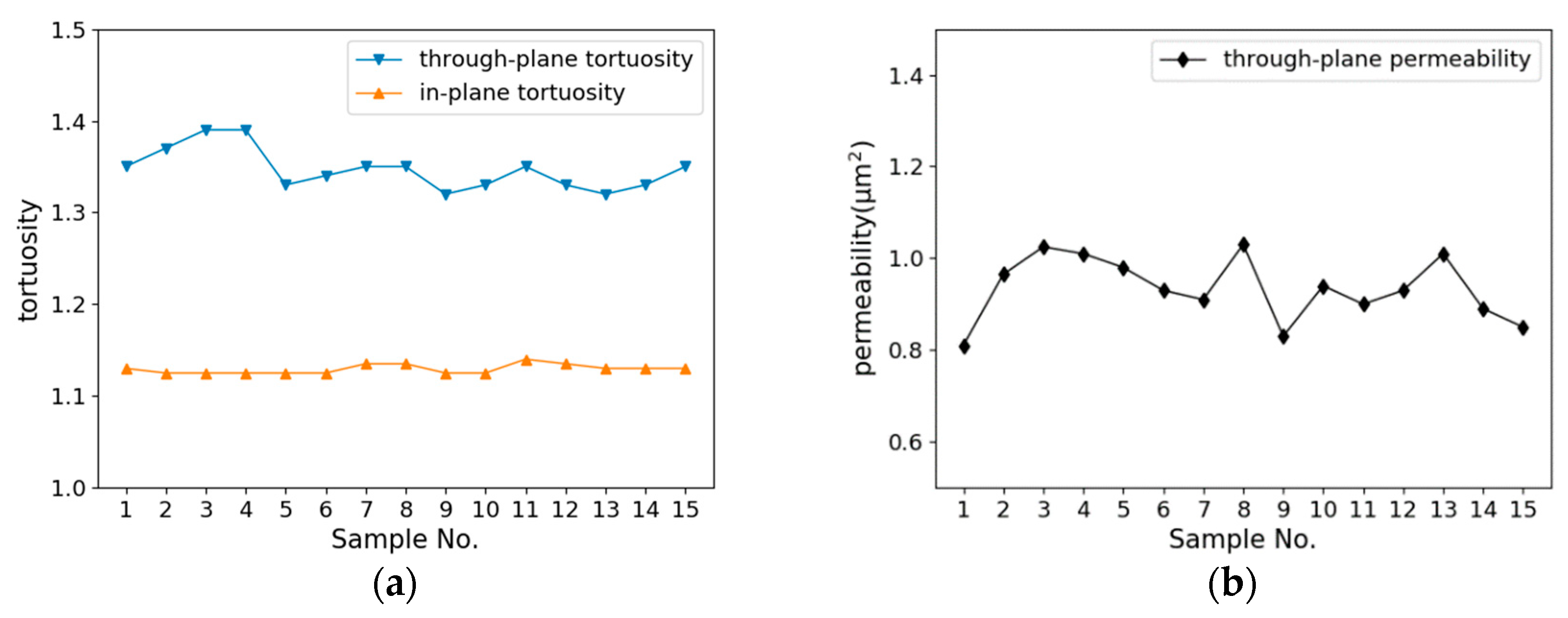
3.1. Calculation Permeability and Tortuosity of the Single Fiber Carbon Cloth Model

According to Salomov’s paper [24], the calculated porosity of his carbon cloth reconstruction model is 0.6892, which is close to the experimental value. Based on the carbon cloth reconstruction method proposed in Section 2.3 and authors’ previous studies, the carbon cloth structure parameters in Table 1 are taken as input, and constructed 15 different carbon cloth samples for modeling. Three samples are chosen from the 15 reconstruction results and are shown in Figure 5. It can be seen that the structure of the carbon cloth sample is a regular woven-type, and the randomness of the fiber distribution is embodied in the elliptical bundle.
The calculation method of permeability based on Lattice Boltzmann method, Navier–Stokes equation, and Darcy’s law and the calculation method of tortuosity based LBM was introduced in detail in our previous paper [26]. Furthermore, some researchers have studied the relationship between the permeability and porosity. For GDL-type materials, Tamadakis and Robertson [27] derive the following equation:
k r 2 = ε 8 ln 2 ε ( ε ε p 1 ε p ) a ( 1 + α ε ε ε p ) 2
where k is the permeability of materials, r is the fiber radius, ε is the porosity, εp is the percolation porosity, and α is an Archie’s law parameter. The value of εp and α will be different for through-plane and in-plane direction. α depends on medium structure and flow direction. For the GDL-type media, the value of εp is 0.11, α is 0.785 for the through-plane direction and 0.521 for the in-plane direction.
As for tortuosity, Koponen et al. [28] proposed the following equation, which has been widely used to verify anisotropic tortuosity prediction in PEMFC models:
τ = 1 + a 1 ε ( ε ε p ) m
where ε is porosity, εp is the percolation threshold, a and m are constants. For through-plane direction and in-plane direction, a and m will take different values.
In this section, authors use the Tamadakis and Robertson equation and the Koponen equation as verifications for the calculated permeability and tortuosity.
Figure 6a,b are plotted from the calculated values of tortuosity and permeability of these 15 samples. The fluid inside the GDL is driven by a pressure gradient along the z-direction. It can be seen from the figure that the tortuosity and permeability of the 15 carbon cloth models vary within a certain range. Table 2 shows the average of these 15 calculations and the values calculated by the Tamadakis and Robertson equation and the Koponen equation. The through-plane tortuosity and permeability calculated by the formulas are slightly different from the calculated value of the model. Considering that the difference is so small, the calculated value of the model can be approximated to be consistent with the formulas.

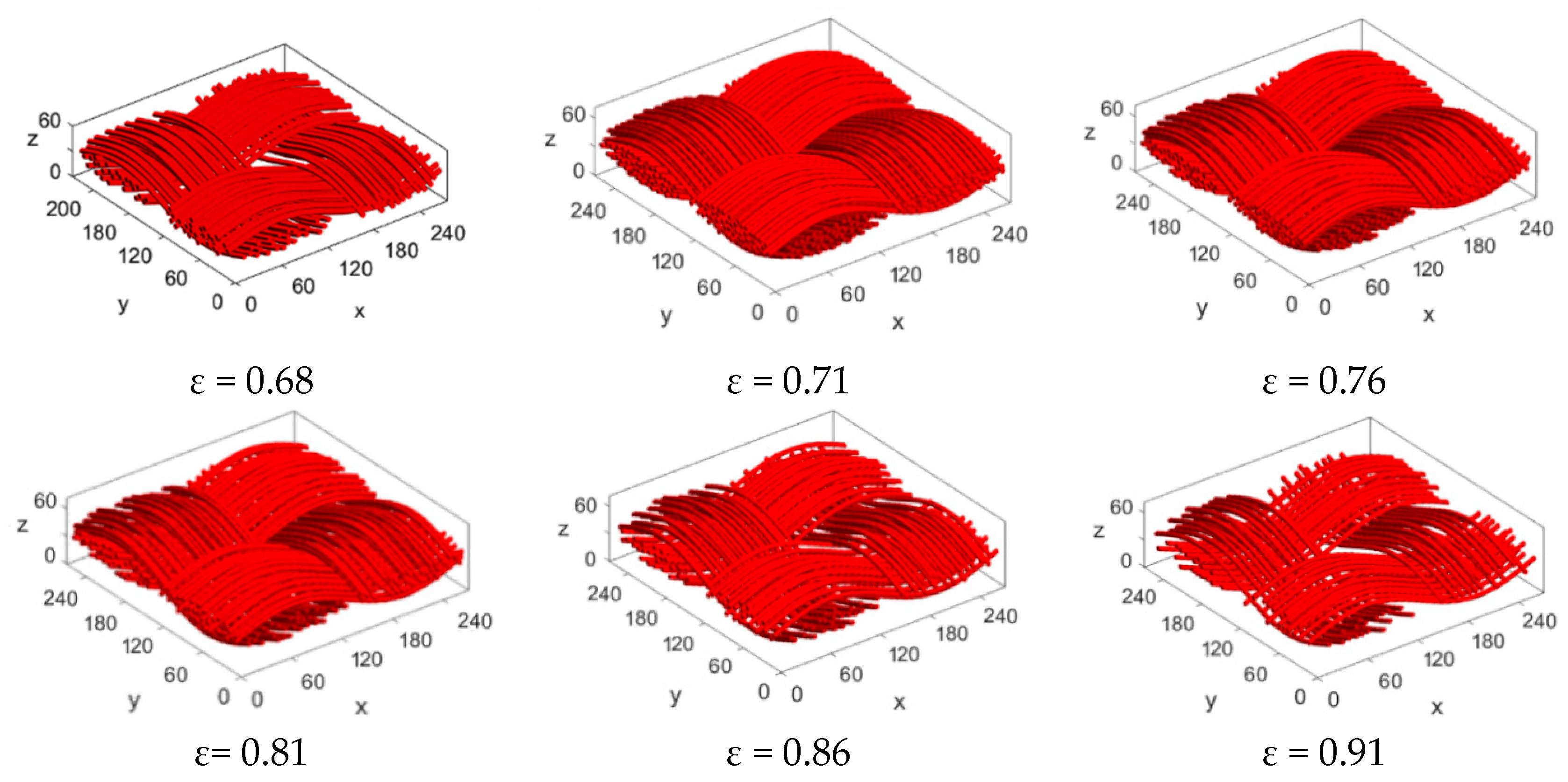
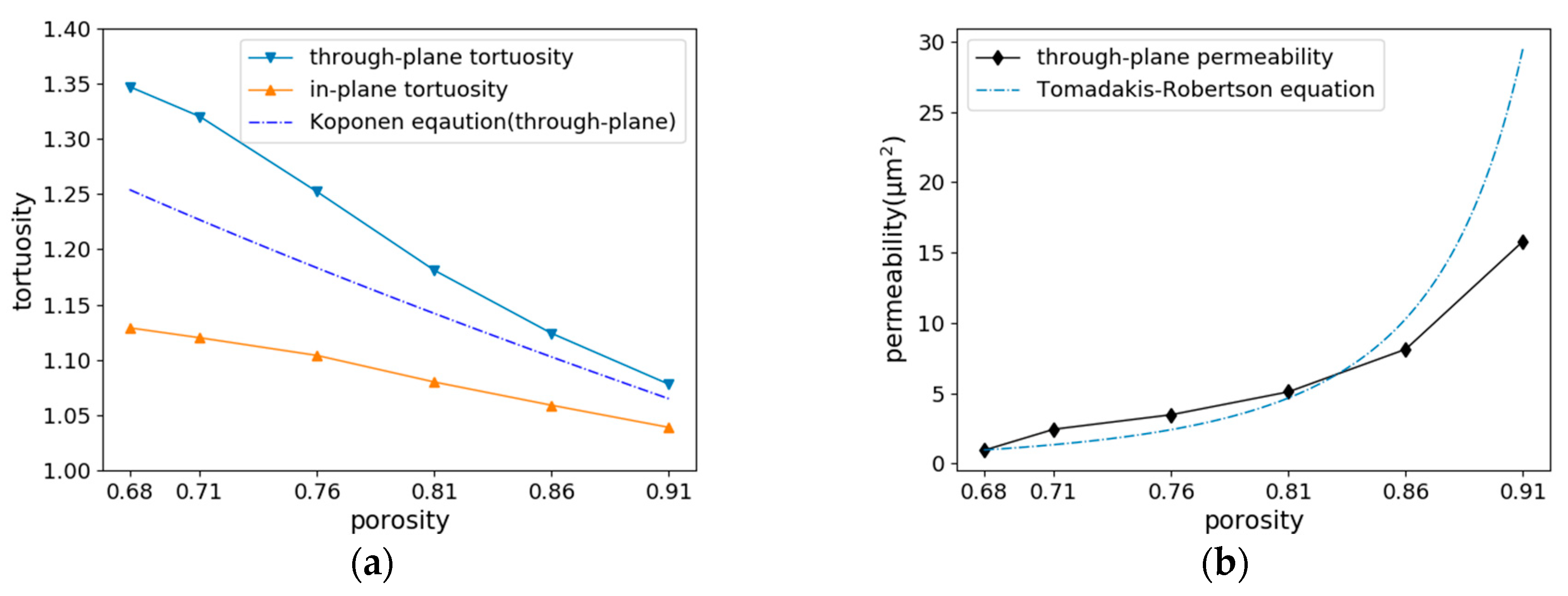
3.2. Calculation of Permeability and Tortuosity for Carbon Cloth Models with the Same Fiber Radius but Different Porosity

Figure 7 shows several 3D visual samples of stochastically reconstructed carbon cloth with different porosities. When other parameters are constant, as the porosity increases, the fiber distribution of the carbon cloth gradually becomes sparse, the pore area increases significantly and the number of fibers reduces. It can be seen in the figure that the carbon cloth model with a porosity greater than 0.91 no longer looks like the actual carbon cloth structure. Although fuel cell is preferring this kind of thin GDL because it has light weight and saves cost on material spending, also it can have more superiority over the water and gas transmission, this material cannot give enough support to the catalyst layer, and the compression resistance is also greatly reduced.
Figure 8a,b are the calculation results of the tortuosity and permeability of the 3D numerical samples of carbon cloth with different porosities. Figure 8a shows the change of tortuosity with different porosity values. In order to ensure a smaller error, each porosity value was used to stochastically constructed six different samples for calculation, and then compared the average values in both through-plane and in-plane directions. It can be seen from the figure that as the porosity increases, the tortuosity along through-direction decreases gradually, same as the Koponen equation, but only a slight decrease along in-plane direction. The reason is that the random distribution of fibers has a great impact on the through-plane direction of carbon cloth, which makes the pore size and pore distribution characteristics between each fiber inconsistent, and it also affects the pore diameter curvature inside the structure. In the range of 0.71–0.86, the tortuosity along through-plane direction decreases greatly, which indicates that the degree of twists of the mass transmission paths on through-plane direction is gradually decreasing. However, when the porosity increases to more than 0.86, the pore structure similarity is higher due to the significant decrease of the fiber numbers and make the tortuosity is almost unchanged.
From Figure 8b, we can find that when the porosity is in the range of 0.68–0.86, the permeability of our samples is in good agreement with the Tamadakis and Robertson equation. However, as the porosity continues to increase, the permeability of our samples remains almost constant and is much smaller than the empirical formula. This may be due to the fact that at high porosity, the models are already difficult to access the actual GDL structure, which makes large errors in calculating the permeability.

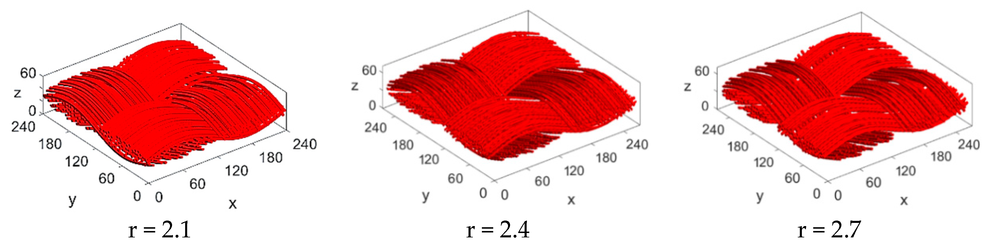
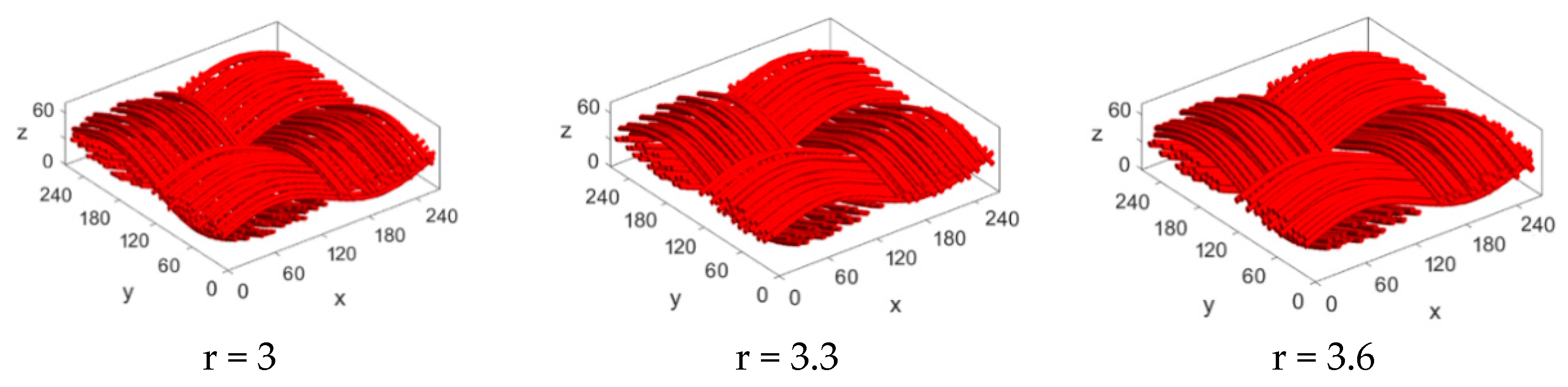
3.3. Calculation of Permeability and Tortuosity for Carbon Cloth Models with the Same Porosity but Different Fiber Radius

Figure 9 shows some 3D visual samples of stochastically reconstructed carbon cloth with different fiber radii. When the other parameters are constant, as the fiber radius increases, the number of fibers contained in the bundle decreases, and the fiber distribution becomes sparser. Compared with the obvious change of the carbon paper model, the regularity of the carbon cloth fiber distribution makes the visual effect of the model be similar, and the change of the pore structure is mainly reflected in the fiber bundle.
Figure 10a,b are the calculation results of the tortuosity and permeability of the 3D numerical model of carbon cloth with different radii. The results show that when the radius increases, the tortuosity along in-plane direction is basically unchanged and the tortuosity along through-plane direction is slightly reduced in the range of 2.1–3.3 μm. When the fiber radius is greater than 3.3 μm, the tortuosity along through-plane direction remains essentially the same. The permeability along through-plane direction gradually increases, which is constant with the trend of Tamadakis and Robertson equation. As the fiber radius becomes larger, the pore size correspondingly becomes larger, too. In the microscopic flow, the fluid has a trend to flow forward larger pores, which shortens the flow path of the fluid and provides better fluidity.

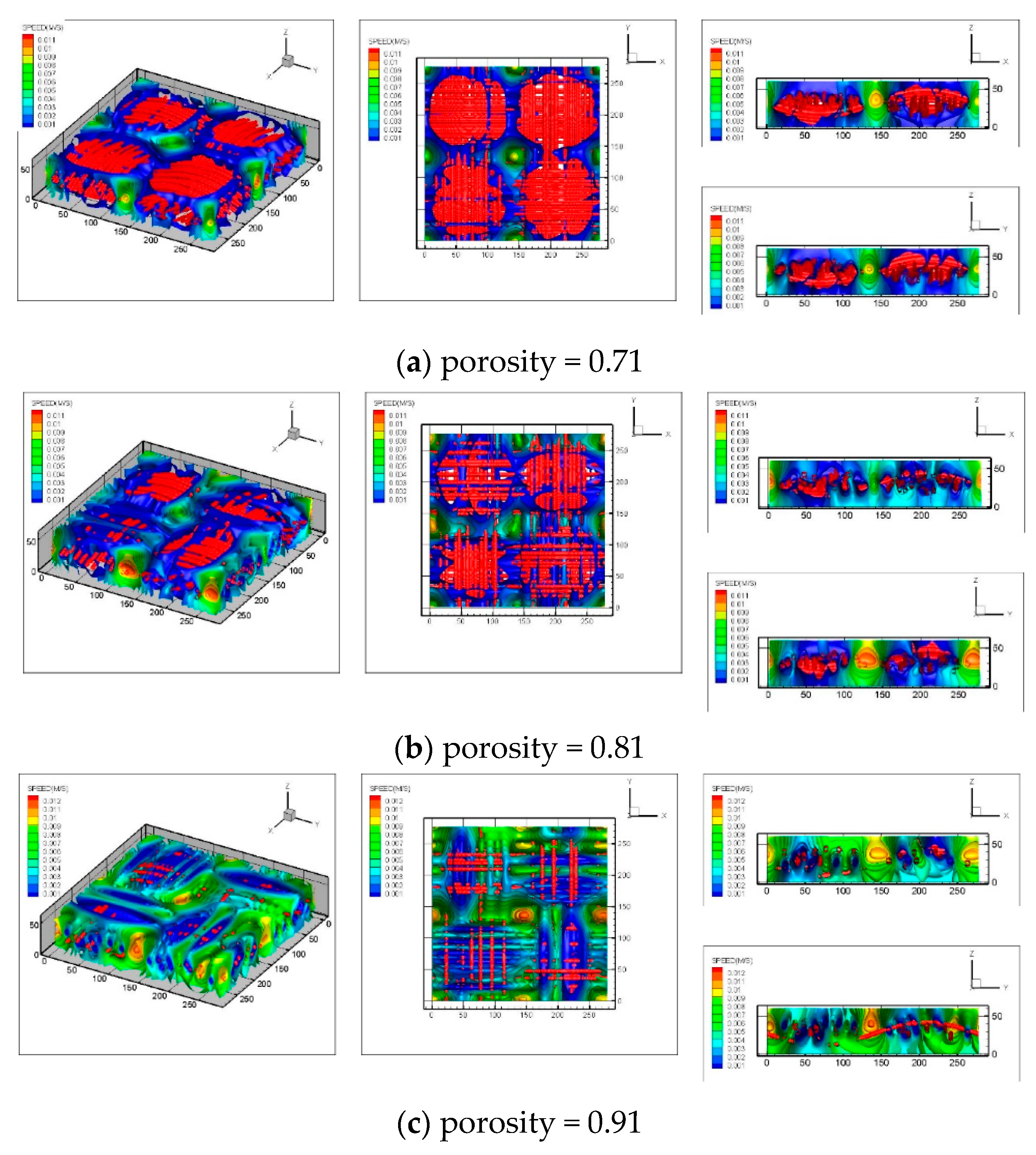
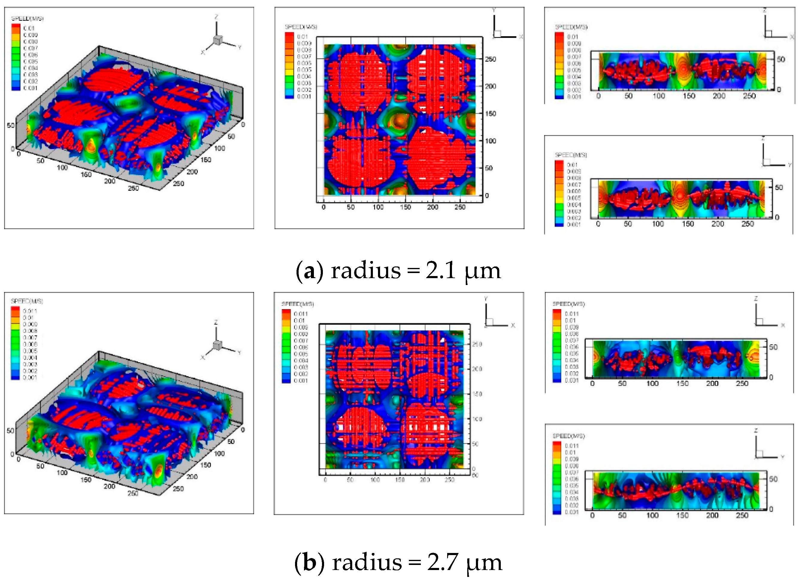
3.4. Velocity Distribution

The velocity distribution of fluid in the porous medium can reflect the penetrability of the medium. To drive the fluid flowing, inlet and output pressure boundaries are applied. Steady water flow in the reconstructed carbon cloth is simulated by applying a constant pressure gradient between the bottom and top along z-direction and the bounce-back method is used. Figure 11a–c shows the three-dimensional velocity distributions in the reconstructed carbon cloth GDLs with different porosities. It can be seen that due to the anisotropy structure of the carbon cloth, the velocity field in it is complicated. The velocity distribution show that the main flow paths were through larger pores because of their less flow resistance. The flow of water was more concentrated at the pores formed by the overlap of fiber bundles, where the velocity was much larger. As the porosity increases, the pore space between the fiber bundles increases correspondingly, and the velocity distribution tends to be uniform. However, for carbon cloth GDL with the porosity of 0.91, the carbon cloth structure is difficult to form, water flow tends to accumulate in the pores due to the excessive porosity. Therefore, for better drainage and avoiding flooding, a porosity of 0.81 is more suitable.
Figure 12a–d shows the three-dimensional flow fields in carbon cloth GDLs with different fiber radii. As shown in the figure, as the radius increases, the pore space in the carbon cloth increases correspondingly, and the velocity distribution becomes more uniform. For the carbon cloth GDL with the fiber radius of 3.6 μm, the pore space is too large. Water tends to accumulate in the pores and the entire GDL is immersed. To avoid such immersion, a fiber radius of 3 μm or slightly more than 3 μm is optimal.

4. Conclusions

In this study, a new carbon cloth GDL stochastic reconstruction model is proposed, assuming that the carbon cloth is woven by sinusoidal elliptical fiber bundles. The major results about this model are as follows:
  • In the GDL model, the fiber radius and fiber distribution are taken as input parameters and all the input parameters are adjustable. The initial model porosity is 0.68 and the initial fiber radius is 3 μm. The model predictions are validated with the tortuosity along both through-plane and in-plane directions and the permeability along through-plane direction.
  • Different structural parameters can be changed individually to analyze its influence on the transmission characteristics of the structure. By changing the porosity and fiber radius, respectively, it is found that with the increase of porosity, the tortuosity in the through-plane direction gradually decreases and in the in-plane direction stays nearly constant. When the porosity is in the range of 0.68–0.86, the permeability in the through-plane direction basically conforms to the calculation results of the empirical equation and increases gradually as the porosity increases. When the fiber radius is changed, as the radius becomes larger, the tortuosity in the through-plane direction slightly decreases while the permeability correspondingly increases.

Author Contributions

Conceptualization, Y.G. and X.W.; Methodology, X.W.; Software, T.J.; Validation, Y.G., T.J. and X.W.; Formal Analysis, T.J.; Investigation, T.J.; Resources, Y.G.; Data Curation, X.W.; Writing-Original Draft Preparation, J.T.; Writing-Review & Editing, Y.G.; Visualization, Y.G.; Supervision, Y.G.; Project Administration, Y.G.; Funding Acquisition, Y.G. All authors have read and agreed to the published version of the manuscript.

Funding

This research was funded by the National Key R&D Program of China, Grant number 2018YFE0105000, Natural Science Foundation of Shanghai (China), Grant number 19ZR1460300 and Special Foundation for State Major Basic Research Program of China, Grant number 2018YFB0104501 and the National Natural Science Foundation of China, Grant number 21506165. And the APC was funded by the National Key R&D Program of China, Grant number 2018YFE0105000.

Conflicts of Interest

We declare that we have no conflicts of interest to this work. We declare that we do not have any commercial or associative interest that represents a conflict of interest in connection with the work submitted.

References

  1. Fadzillah, D.; Rosli, M.; Talib, M.; Kamarudin, S.; Daud, W. Review on microstructure modelling of a gas diffusion layer for proton exchange membrane fuel cells. Renew. Sustain. Energy Rev. 2017, 77, 1001–1009. [Google Scholar] [CrossRef]
  2. El-Kharouf, A.; Mason, T.J.; Brett, D.J.; Pollet, B.G. Ex-situ characterisation of gas diffusion layers for proton exchange membrane fuel cells. J. Power Sources 2012, 218, 393–404. [Google Scholar] [CrossRef] [Green Version]
  3. Park, S.; Popov, B.N. Effect of a GDL based on carbon paper or carbon cloth on PEM fuel cell performance. Fuel 2011, 90, 436–440. [Google Scholar] [CrossRef]
  4. Inoue, G.; Yoshimoto, T.; Matsukuma, Y.; Minemoto, M. Development of simulated gas diffusion layer of polymer electrolyte fuel cells and evaluation of its structure. J. Power Sources 2008, 175, 145–158. [Google Scholar] [CrossRef]
  5. Schulz, V.P.; Becker, J.; Wiegmann, A.; Mukherjee, P.P.; Wang, C.-Y. Modeling of Two-Phase Behavior in the Gas Diffusion Medium of PEFCs via Full Morphology Approach. J. Electrochem. Soc. 2007, 154, B419–B426. [Google Scholar] [CrossRef]
  6. Mukherjee, P.P.; Kang, Q.; Wang, C.-Y. Pore-scale modeling of two-phase transport in polymer electrolyte fuel cells—progress and perspective. Energy Environ. Sci. 2011, 4, 346–369. [Google Scholar] [CrossRef]
  7. Oostrom, M.; Lenhard, R. Comparison of relative permeability-saturation-pressure parametric models for infiltration and redistribution of a light nonaqueous-phase liquid in sandy porous media. Adv. Water Resour. 1998, 21, 145–157. [Google Scholar] [CrossRef]
  8. Wang, Z.H.; Wang, C.Y.; Chen, K.S. Two-phase flow and transport in the air cathode of proton exchange membrane fuel cells. J. Power Sources 2001, 94, 40–50. [Google Scholar] [CrossRef] [Green Version]
  9. Hinebaugh, J.; Bazylak, A. Stochastic modeling of polymer electrolyte membrane fuel cell gas diffusion layers—Part 1: Physical characterization. Int. J. Hydrog. Energy 2017, 42, 15861–15871. [Google Scholar] [CrossRef]
  10. Hinebaugh, J.; Gostick, J.; Bazylak, A. Stochastic modeling of polymer electrolyte membrane fuel cell gas diffusion layers—Part 2: A comprehensive substrate model with pore size distribution and heterogeneity effects. Int. J. Hydrog. Energy 2017, 42, 15872–15886. [Google Scholar] [CrossRef]
  11. Shojaeefard, M.; Molaeimanesh, G.; Nazemian, M.; Moqaddari, M. A review on microstructure reconstruction of PEM fuel cells porous electrodes for pore scale simulation. Int. J. Hydrog. Energy 2016, 41, 20276–20293. [Google Scholar] [CrossRef]
  12. Becker, J.; Flückiger, R.; Reum, M.; Büchi, F.N.; Marone, F.; Stampanoni, M. Determination of Material Properties of Gas Diffusion Layers: Experiments and Simulations Using Phase Contrast Tomographic Microscopy. J. Electrochem. Soc. 2009, 156, B1175. [Google Scholar] [CrossRef]
  13. Thiedmann, R.; Fleischer, F.; Hartnig, C.; Lehnert, W.; Schmidt, V. Stochastic 3D Modeling of the GDL Structure in PEMFCs Based on Thin Section Detection. J. Electrochem. Soc. 2008, 155, B391. [Google Scholar] [CrossRef]
  14. Koido, T.; Furusawa, T.; Moriyama, K. An approach to modeling two-phase transport in the gas diffusion layer of a proton exchange membrane fuel cell. J. Power Sources 2008, 175, 127–136. [Google Scholar] [CrossRef]
  15. Ostadi, H.; Rama, P.; Liu, Y.; Chen, R.; Zhang, X.; Jiang, K. Nanotomography based study of gas diffusion layers. Microelectron. Eng. 2010, 87, 1640–1642. [Google Scholar] [CrossRef] [Green Version]
  16. Ostadi, H.; Rama, P.; Liu, Y.; Chen, R.; Zhang, X.; Jiang, K. Influence of threshold variation on determining the properties of a polymer electrolyte fuel cell gas diffusion layer in X-ray nano-tomography. Chem. Eng. Sci. 2010, 65, 2213–2217. [Google Scholar] [CrossRef] [Green Version]
  17. Rama, P.; Liu, Y.; Chen, R.; Ostadi, H.; Jiang, K.; Zhang, X.; Gao, Y.; Grassini, P.; Brivio, D. Determination of the anisotropic permeability of a carbon cloth gas diffusion layer through X-ray computer micro-tomography and single-phase lattice Boltzmann simulation. Int. J. Numer. Methods Fluids 2011, 67, 518–530. [Google Scholar] [CrossRef] [Green Version]
  18. Rama, P.; Liu, Y.; Chen, R.; Ostadi, H.; Jiang, K.; Gao, Y.; Zhang, X.; Brivio, D.; Grassini, P. A Numerical Study of Structural Change and Anisotropic Permeability in Compressed Carbon Cloth Polymer Electrolyte Fuel Cell Gas Diffusion Layers. Fuel Cells 2011, 11, 274–285. [Google Scholar] [CrossRef]
  19. García-Salaberri, P.A.; Hwang, G.; Vera, M.; Weber, A.Z.; Gostick, J.T. Effective diffusivity in partially-saturated carbon-fiber gas diffusion layers: Effect of through-plane saturation distribution. Int. J. Heat Mass Transf. 2015, 86, 319–333. [Google Scholar] [CrossRef] [Green Version]
  20. García-Salaberri, P.A.; Gostick, J.T.; Hwang, G.; Weber, A.Z.; Vera, M. Effective diffusivity in partially-saturated carbon-fiber gas diffusion layers: Effect of local saturation and application to macroscopic continuum models. J. Power Sources 2015, 296, 440–453. [Google Scholar] [CrossRef] [Green Version]
  21. Schladitz, K.; Peters, S.; Reinel-Bitzer, D.; Wiegmann, A.; Ohser, J. Design of acoustic trim based on geometric modeling and flow simulation for non-woven. Comput. Mater. Sci. 2006, 38, 56–66. [Google Scholar] [CrossRef] [Green Version]
  22. Froning, D.; Yu, J.; Gaiselmann, G.; Reimer, U.; Manke, I.; Schmidt, V.; Lehnert, W. Impact of compression on gas transport in non-woven gas diffusion layers of high temperature polymer electrolyte fuel cells. J. Power Sources 2016, 318, 26–34. [Google Scholar] [CrossRef]
  23. Froning, D.; Yu, J.; Reimer, U.; Lehnert, W. Stochastic Analysis of the Gas Flow at the Gas Diffusion Layer/Channel Interface of a High-Temperature Polymer Electrolyte Fuel Cell. Appl. Sci. 2018, 8, 2536. [Google Scholar] [CrossRef] [Green Version]
  24. Salomov, U.R.; Chiavazzo, E.; Asinari, P. Pore-scale modeling of fluid flow through gas diffusion and catalyst layers for high temperature proton exchange membrane (HT-PEM) fuel cells. Comput. Math. Appl. 2014, 67, 393–411. [Google Scholar] [CrossRef] [Green Version]
  25. Gao, Y.; Zhang, X.; Rama, P.; Chen, R.; Ostadi, H.; Jiang, K. An Improved MRT Lattice Boltzmann Model for Calculating Anisotropic Permeability of Compressed and Uncompressed Carbon Cloth Gas Diffusion Layers Based on X-Ray Computed Micro-Tomography. J. Fuel Cell Sci. Technol. 2012, 9, 041010. [Google Scholar] [CrossRef]
  26. Gao, Y.; Montana, A.; Chen, F. Evaluation of porosity and thickness on effective diffusivity in gas diffusion layer. J. Power Sources 2017, 342, 252–265. [Google Scholar] [CrossRef]
  27. Tomadakis, M.M.; Robertson, T.J. Viscous Permeability of Random Fiber Structures: Comparison of Electrical and Diffusional Estimates with Experimental and Analytical Results. J. Compos. Mater. 2005, 39, 163–188. [Google Scholar] [CrossRef]
  28. Koponen, A.; Kataja, M.; Timonen, J. Tortuous flow in porous media. Phys. Rev. E 1996, 54, 406–410. [Google Scholar] [CrossRef]
Figure 1. The bunched fiber sample of carbon cloth gas diffusion layer (GDL). (a) A primitive cell of carbon cloth GDL and (b) the concatenation of primitive cells.
Energies 13 00572 g001
Figure 2. Geometrical relation between abscissa and minimum distance.
Energies 13 00572 g002
Figure 3. Flow chart of reconstruction process of the single fiber carbon cloth.
Energies 13 00572 g003
Figure 4. Images of carbon cloth GDL samples. (a) SEM image of carbon cloth GDL [25]. (b) The single-fiber carbon cloth GDL and (c) slices of the reconstructed model.
Energies 13 00572 g004
Figure 5. Three-dimensional stochastically reconstructed carbon cloth samples.
Energies 13 00572 g005
Figure 6. Calculated (a) tortuosity and (b) permeability of samples.
Energies 13 00572 g006
Figure 7. Carbon cloth models with different porosities (fiber radius = 3 μm).
Energies 13 00572 g007
Figure 8. Calculated (a) tortuosity and (b) permeability of models with different porosities.
Energies 13 00572 g008
Figure 9. Carbon cloth models with different fiber radii (porosity = 0.81).
Energies 13 00572 g009aEnergies 13 00572 g009b
Figure 10. Calculated (a) tortuosity and (b) permeability of models with different fiber radii.
Energies 13 00572 g010
Figure 11. The simulated velocity fields of carbon cloth GDLs with different porosities. (fiber radius = 3 μm). (a) porosity = 0.71 (b) porosity = 0.81 (c) porosity = 0.91.
Energies 13 00572 g011
Figure 12. The simulated velocity fields of carbon cloth GDLs with different fiber radii (porosity = 0.81). (a) radius = 2.1 μm (b) radius = 2.7 μm (c) radius = 3 μm (d) radius = 3.6 μm.
Energies 13 00572 g012aEnergies 13 00572 g012b
Table 1. Input parameters of stochastically reconstructed carbon cloth model.
ModelPorosityFiber Radius/μmEllipse Size/μmThickness/μm
Single fiber model of carbon cloth GDL0.683Semi-major/semi-minor axis 60/1260
Table 2. Average of calculation permeability and tortuosity.
Through-Plane TortuosityIn-Plane TortuosityThrough-Plane Tortuosity (Koponen Equation)Through-Plane Permeability (μm2)Through-Plane Permeability (μm2) (Tamadakis and Robertson Equation)
1.3471.1291.2540.9341.077

