Article

An Intelligent Model to Predict Energy Performances of Residential Buildings Based on Deep Neural Networks

by
Azadeh Sadeghi
1,
Roohollah Younes Sinaki
1,
William A. Young II
2,* and
Gary R. Weckman
1
1
Industrial and Systems Engineering, Russ College of Engineering, Ohio University, Athens, OH 45701, USA
2
Analytics and Information Systems, College of Business, Ohio University, Athens, OH 45701, USA
*
Author to whom correspondence should be addressed.
Energies 2020, 13(3), 571; https://doi.org/10.3390/en13030571
Submission received: 18 December 2019 / Revised: 15 January 2020 / Accepted: 22 January 2020 / Published: 24 January 2020
(This article belongs to the Special Issue Optimal Design and Operation of Sustainable Energy Systems)

Abstract

:
As the level of greenhouse gas emissions increases, so does the importance of the energy performance of buildings (EPB). One of the main factors to measure EPB is a structure’s heating load (HL) and cooling load (CL). HLs and CLs depend on several variables, such as relative compactness, surface area, wall area, roof area, overall height, orientation, glazing area, and glazing area distribution. This research uses deep neural networks (DNNs) to forecast HLs and CLs for a variety of structures. The DNNs explored in this research include multi-layer perceptron (MLP) networks, and each of the models in this research was developed through extensive testing with a myriad number of layers, process elements, and other data preprocessing techniques. As a result, a DNN is shown to be an improvement for modeling HLs and CLs compared to traditional artificial neural network (ANN) models. In order to extract knowledge from a trained model, a post-processing technique, called sensitivity analysis (SA), was applied to the model that performed the best with respect to the selected goodness-of-fit metric on an independent set of testing data. There are two forms of SA—local and global methods—but both have the same purpose in terms of determining the significance of independent variables within a model. Local SA assumes inputs are independent of each other, while global SA does not. To further the contribution of the research presented within this article, the results of a global SA, called state-based sensitivity analysis (SBSA), are compared to the results obtained from a traditional local technique, called sensitivity analysis about the mean (SAAM). The results of the research demonstrate an improvement over existing conclusions found in literature, which is of particular interest to decision-makers and designers of building structures.

1. Introduction

Energy waste is a growing concern, given its negative effects on the environment. As a result, decision-makers should pay close attention to energy efficiency. According to the International Energy Agency (IEA) [1], buildings are the largest energy-consuming sector. In 2018, the International Energy Agency (IEA) [2] reported a 3% annual increase in building energy demand, due to the continuous increase in global access to energy, greater access to energy devices, and global growth in building floor area. Recent studies indicate that the thermal load efficiency in buildings is 33%, buildings consume more than 50% of the global energy, and carbon emitted by buildings accounts for 30% of the global carbon emissions [3]. Given this impact, increasing the efficiency of energy performance buildings (EPB) has captured the attention of many researchers. Being able to accurately predict EPB has significant consequences for the world, including being able to better reduce electricity consumption, manage energy demand by keeping a better balance between energy production and demand, reduce operational costs, and reduce carbon emissions ([4,5]). Domestic and international factors affect the energy consumption of residual buildings [6]. The energy load of residential buildings is defined as the amount of electricity or fuel that a building needs in order to ensure the residents’ comfort and safety. Heating load (HL) is the heat transfer within the building and between the building and the external environment when the building is cold. Similarly, cooling load (CL) is defined as the cold transfer within the building and between the building and the external environment when the building is hot. In addition to the temperature, the thermal load controls the moisture (e.g., latent heat) [3].
Estimating thermal load requires knowing a significant amount about a building’s characteristics before it is evaluated. There are four significant tools mainly used to forecast EPB. These tools include engineering calculations, simulation modeling, statistical modeling, and machine learning [7]. Engineering calculations apply laws and complex mathematics to estimate energy consumption. Simulation tools have been widely applied in order to simulate energy performance with respect to a pre-determined status; however, it requires specific knowledge and skills, and it is time-consuming. Bagheri et al. [8] reviewed simulation techniques, software, and drawbacks in the area of energy performance. Statistical methods frequently apply regression when modeling EPB. Machine learning is mostly categorized as a subsection of statistical methods, but it does have the capability to learn from the existing data in order to forecast the desired outputs. Machine learning provides options for designers to quickly analyze the effects of modifying parameters and performing statistical analysis. Modeling EPB with artificial intelligence and machine-learning methods has become more popular in recent years, given the growing amount of EPB data that is available to the public. Machine-learning methods, such as artificial neural networks (ANNs), support vector machines, Gaussian-based regression, and clustering, have been applied to specific models of HL and CL [7].
Machine learning applies a specific algorithm to a dataset, and based on the methodology, the algorithm can “learn” from the given data. Machine-learning algorithms are mainly classified into two categories: supervised learning and unsupervised learning. In supervised learning, the expected output variables are available. This is not like unsupervised learning since for the latter, a specific labeled output does not exist. The focus of the current research is on supervised learning since the available dataset is labeled. Among supervised learning techniques, ANNs have attracted attention because of their capability to model non-linear relationships within data. In other words, activation functions in ANNs can forecast outputs which have non-linear relationships with various inputs. ANNs are a form of main machine learning that has been applied in EPB [7]. ANNs have many structures. Three commonly used ANN architectures include feed-forward, radial basis function, and recurrent networks. In this study, feedforward multi-layer perceptron (MLP) ANNs are applied. In MLPs, data travels in multiple layers in a single direction. A simple MLP model includes an input layer, a hidden layer, and an output layer. In this structure, the model consists of neurons that act as weighted transfer functions. Even though simple MLP designs are quite powerful, increasing the number of hidden layers can help model more complex data. ANNs including a significant number of hidden layers are referred to as deep neural networks (DNNs), and the process of training the model is called deep learning (DL).
An ANN is a powerful tool for handling large and complex datasets, although it has been criticized by researchers due to a lack of model transparency [9]. In order to adequately examine the relationship between variables, sensitivity analysis (SA) is widely applied. Eliminating insignificant inputs in an ANN has been shown to increase forecasting accuracies, which also simplifies and improves the knowledge that can be extracted from an accurate model [10]. One of the traditional techniques is sensitivity analysis about the mean (SAAM), which is categorized as a local sensitivity technique. In SAAM, the changing of dependent variables is captured while individual independent variables vary across their sample range and the rest of the inputs are held to their sample means [11]. SAAM captures cause-and-effect relationships between dependent and independent variables. The advantages of this method include easy implementation, simple interpretation, and application, along with quality statistical analysis [12,13]. On the other hand, global SA techniques, such as state-based sensitivity analysis (SBSA), take a different approach. For example, in SBSA, as independent variables are individually varied, all other independent variables are simultaneously adjusted in order to capture the resultant change in the dependent attribute [9].
There are many factors that can affect the HL and the CL in residential buildings. For example, user behavior profiles would inevitably yield high variations of HLs and CLs within structures. Thus, inputs related to the use of structures could play a critical role when trying to build predictive models for HLs and CLs. However, the focus of this study specifically involves relative compactness, surface area, wall area, roof area, overall height, building orientation, glazing area, and glazing distribution. Tsanas and Xifara [14] identified these factors by simulating different building shapes in order to forecast EPB. According to Tsanas and Xifara [14], simulation tools play a critical role in facilitating the design of structures. Moreover, simulation can often accurately reflect actual measurements [15]. This paper applies and compares ANN and DNN techniques to the available dataset in order to forecast the energy performance of residential buildings. To date, the capability of DNNs in forecasting EPB has not been thoroughly explored. In this regard, DNNs make an ideal choice to forecast HL and CL, due to highly non-linear relationships observed in the dataset. Experiments are conducted by considering ANNs, implementing different numbers of layers in the DNN, using different numbers of processing elements, and using data preprocessing techniques that include normalization, randomization, and moving averages (MAs). ANN models were developed to forecast HLs and CLs individually, as well as predict HLs and CLs simultaneously within a single ANN structure. In order to evaluate the performance of the proposed models, a prediction interval analysis was performed. Consequently, after identifying the best-performing model on an independent testing dataset, both SAAM and SBSA were conducted. The significance of this research can help engineers understand key structural considerations so that they can construct more energy-efficient buildings.
The organization of this paper includes a description of both background literature and related work on EPB and the applied machine-learning techniques in Section 2. Section 3 discusses the methodological approach by describing the characteristics of the dataset and the framework used to process the data. Section 4 shows the results after applying the developed framework, local and global SA, and statistical analysis. Section 5 focuses on the conclusion.

2. Literature Review
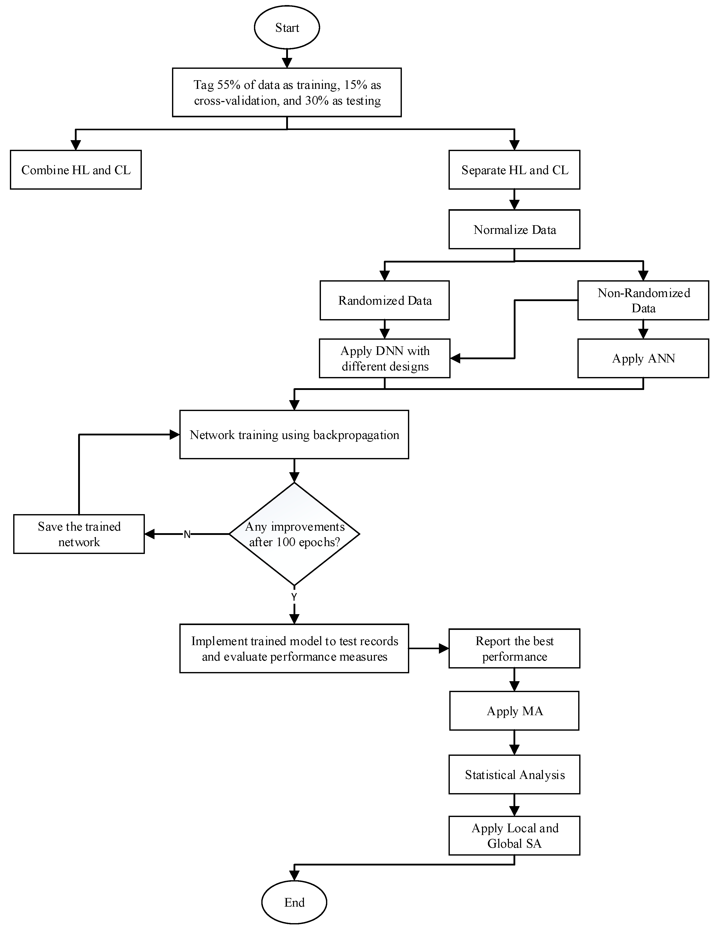
In the literature reviewed for this research, buildings are often categorized into four main groups: commercial, educational, residential, and mixed-use. One discovery showed that residential buildings incorporate 30% of the literature on building energy models [16]. Forecasts for thermal load in residual buildings can be made for both short-term and long-term periods of time [17]. In order to forecast HL and CL in residual buildings in the long-term, Tsanas and Xifara [14] simulated 12 different building shapes in a software program called Ecotects. When considering all the different combinations of input variables, 768 building shapes were created. Heating, ventilation, and air conditioning (HVAC) regulations were followed while simulating building shapes. This dataset has become popular in the area of EPB, and different machine-learning techniques have been applied for accurate forecasting. Table 1 summarizes the literature that is based on the influential contributions from Tsanas and Xifara [14]. Though the dataset is based on simulated data and lacks certain inputs related to the use of the structures that might be included in other datasets, the dataset is publicly available and has been widely used within the research community that explores data-driven applications within energy studies. Given the significance that simulation plays within designing building structures, the significance of this dataset should not go unrecognized. The table categorizes the literature that has used this dataset by identifying the applied machine-learning method, the applied method to identify significant inputs, whether HL and CL were considered combined or separated when forecasting EPB, and performance measures used to indicate the accuracy of the machine-learning method. The nomenclatures used in Table 1 are summarized below in Table 1.
Table 1 shows the publications that applied machine-learning techniques to the dataset created by Tsanas and Xifara [14]. Tsanas and Xifara [14] performed a comprehensive statistical analysis that consisted of density plots and scatter-plots. The result of the statistical analysis indicates the non-linear nature of the problem and the necessity of applying machine-learning algorithms that capture this nature. For this reason, an ANN is one of the most appropriate machine-learning methods for the current dataset. According to Table 1, some papers specifically applied ANN to the dataset (Ahmed et al. [20]; Nwulu [28]), while others applied the ensemble approach by incorporating ANNs (Chou and Bui [18]; Sonmez et al. [21]; Naji et al. [25]; Nilashi et al. [27]). To the best of the authors’ knowledge, Sekha et al. [4] is the only paper that applied DNNs to forecast HL and CL. The performance of DNNs is compared with other machine-learning algorithms, including Gaussian process regression (GPR) and minimax probability machine regression (MPMR). It was concluded that the overall performance of GPR and MPMR surpasses that of the other methods. However, Sekhar et al. [4] did not discuss the characteristics of the applied DNN models, such as the number of layers, the number of processing elements, and activation functions.
While applying machine-learning algorithms on a dataset, it is important to recognize the significant and insignificant inputs. By eliminating insignificant inputs, the efficiency of the model will improve. According to Roy et al. [3], multivariate adaptive regression splines (MARS) is a non-parametric regression model that identifies the importance of each parameter before it is processed by a machine-learning technique. MARS can be used along with hybrid models in order to improve efficiency. Another SA technique is principal component analysis (PCA), which identifies significant inputs in a dataset, reduces the dimension of the data, and eliminates the problem of multi-collinearity. Nilashi et al. [27] states that PCA has four objectives: extracting important information, compressing data, simplifying the descriptions, and analyzing the structure of observations. According to Table 1, most of the reviewed papers did not apply any SA techniques on the dataset.
Quantitative SA techniques are categorized as local and global [33]. Ardjmand et al. [9] criticized local SAs because they did not capture non-linear relationships or multicollinearity, and they did not assume input variables were independent of each other. In other words, changing the value of one of the input variables will affect the value of other inputs; therefore, assuming fixed values for other inputs in local SAs are not realistic. Global SA alters the value of the desired input while multidimensionality takes the average of other inputs [34]. Depending upon the objective of the SA, Ardjmand et al. [9] categorized global SA techniques into screening, regression-based, and variance-based approaches, and extended traditional SA into SBSA, which is classified as a regression-based approach.
There are several decisions that affect the performance of a mathematical model. In order to forecast EPB, HL and CL can be combined or separated outputs. Most of the reviewed articles considered HL and CL separately, but none of them compared two scenarios in a single study. Another important criterion to improve the quality of a predictive model is data pre-processing. By plotting the EPB data, Kumar et al. [31] indicated that none of the inputs follow a normal distribution. Therefore, normalizing inputs before processing them should improve the performance of the model. None of the reviewed papers applied moving average (MA) or randomization as preprocessing techniques in order to improve the predictive performances of a model. Table 1 summarizes the performance measures that were found in the literature. Notably, R2, MAE, and RMSE were among the most popular goodness-of-fit statistics used by researchers.
A review of the literature reveals different machine-learning techniques that were applied to forecast HL and CL for the dataset created by Tsanas and Xifara [14]. The main oversight found in the literature was the lack of attention to the capability of DNNs to forecast CL and HL. This study evaluates the performance of DNNs by exploring different characteristics of a network structure, including the number of hidden layers and the number of processing elements. The second gap that was identified was the lack of preprocessing methods that were used to model HL and CL. In fact, very little of the cited literature used normalization techniques, and none of the previous research included the use of MAs or randomization when preprocessing data. This study used normalization, randomization, and MAs as data preprocessing techniques. The third area overlooked was the possibility of combining or separating outputs of the model, which is fulfilled in this research paper. Finally, the lack of application of SA techniques to identify the importance of each input and examine the effect of those inputs on forecasting accuracy motivated the authors to apply and compare the performance of SAAM as well as SBSA. In addition to improving forecasting accuracy, SA provides a deeper insight with respect to the knowledge that can be extracted from an accurate model, and which later can be considered by building designers in order to construct energy-efficient buildings.

3. Methodology

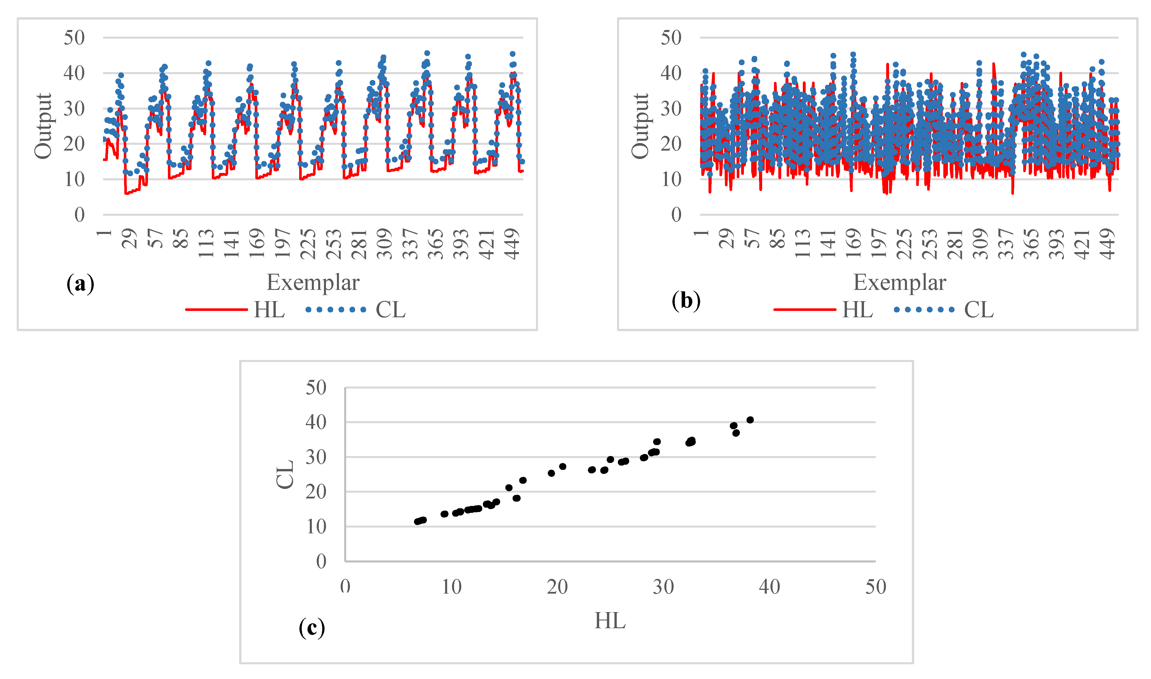
3.1. Description of the Dataset

The characteristics of the dataset used for this research are identical to that of Tsanas and Xifara [14]. Using elementary cubes, 12 building forms were simulated, each of which contained 18 cubes. The buildings’ total volume was 771.75 m3. Building forms have the associated relative compactness (RC) Relative compactness is calculated by comparing the areas of the building shapes to the area of a reference shape when the volumes of the building and the reference shapes are equal [18].
Similar materials were evaluated as U-values and provided for each building. A U-value measures heat transfer and indicates the quality of insulation. The unit for a U-value is Watts-Per-Meter-Square-Kelvin (W/m2 K). Architecture characteristics and associated U-values included walls (1.780), floors (0.860), roofs (0.500), and windows (2.260). The dataset consisted of residential buildings that are located in Athens, Greece. The internal design characteristics included 0.6 clo (c.f. amount of clothing required by a person in a comfortable condition with a temperature of 21 °C—One clo is thermal insulation which is comfortable for a resting man in a specific weather condition) for clothing, 60% of humidity, 0.3 m/s airspeed, and a 300 Lux lighting level. The thermal properties had a 95% efficiency with a thermostat range of 19–24 °C and were operating for 15–20 h on weekdays and 10–20 h on weekends. Three types of glazing areas were used according to what percentage they took up of the total floor area, with 10%, 25%, and 40% being used. There were five different scenarios for the glazing area. These scenarios included: (1) uniform, with 25% glazing on each side, (2) north, with 55% glazing on the north side and 15% glazing on each of the other sides, (3) east, with 55% glazing on the east side and 15% glazing on each of the other sides, (4) south, with 55% glazing on the south side and 15% glazing on each of the other sides, and (5) west, with 55% glazing on the west side and 15% glazing on each of the other sides. Furthermore, there were some buildings with no glazing area at all. There are four orientations represented by 2, 3, 4, and 5, which indicate north facing, south facing, east facing, and west facing, respectively.
The dataset included twelve building forms with three glazing areas, five glazing area distributions, and four orientations, which equated to 720 samples. However, if we included the twelve buildings that did not have glazing with four orientations, the dataset consisted of 768 buildings with their respective HL and CL values. The dataset is freely available at the Center of machine-learning and intelligent systems repository [35].
Table 2 summarizes the characteristics of the input and output variables. The dataset contained eight attributes as inputs and two response variables as outputs. The table shows each variable’s observed range of values.
Actual and randomized measurements of HL and CL for training records are plotted in Figure 1. As shown in Figure 1a,b, output variables were highly correlated with each other both before and after randomization. Figure 1c shows the correlation in a scatter plot. In other words, HL and CL follow similar trends. For instance, if a specific configuration of inputs results in a high HL, it will also result in a high CL.

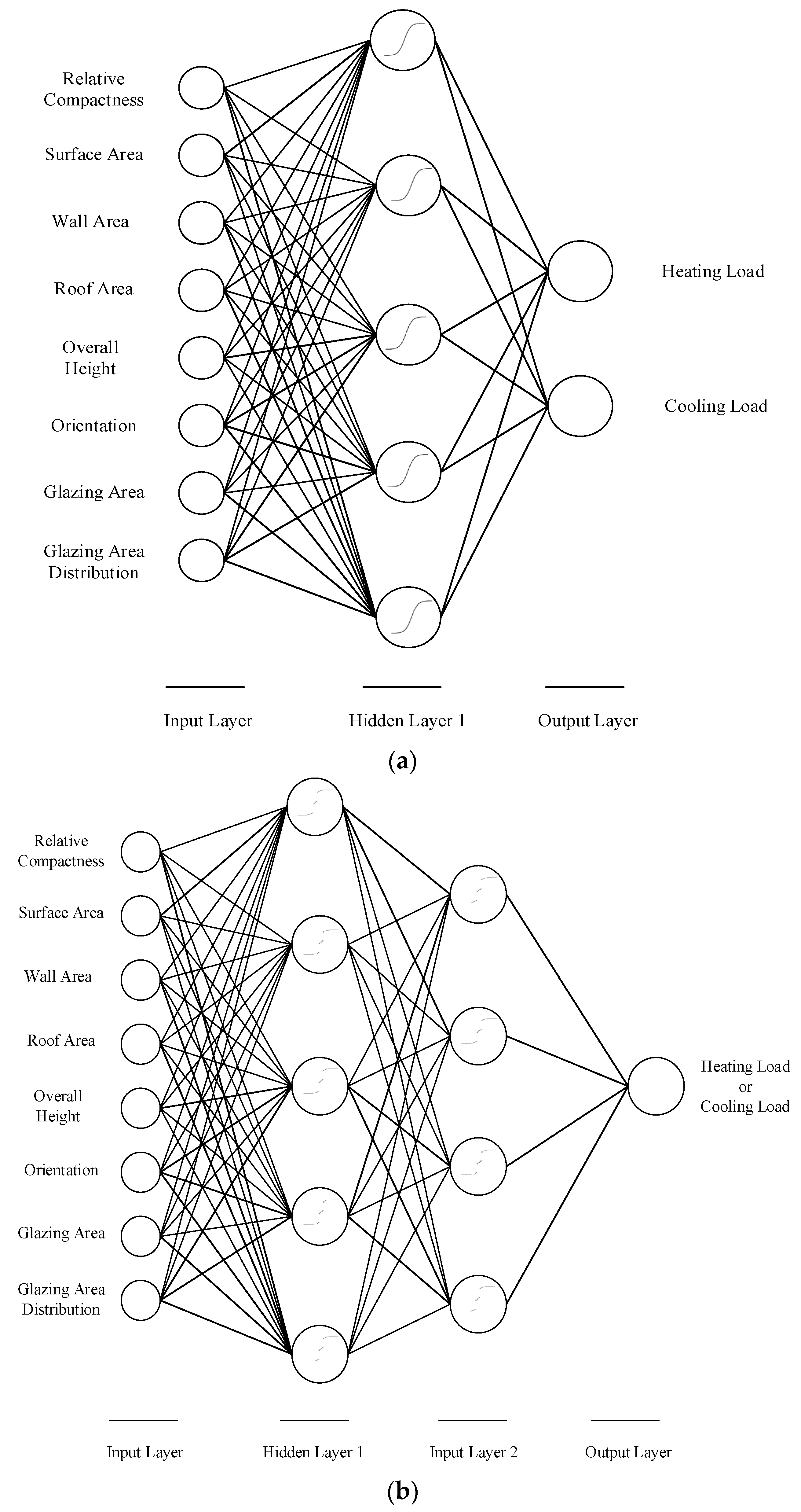
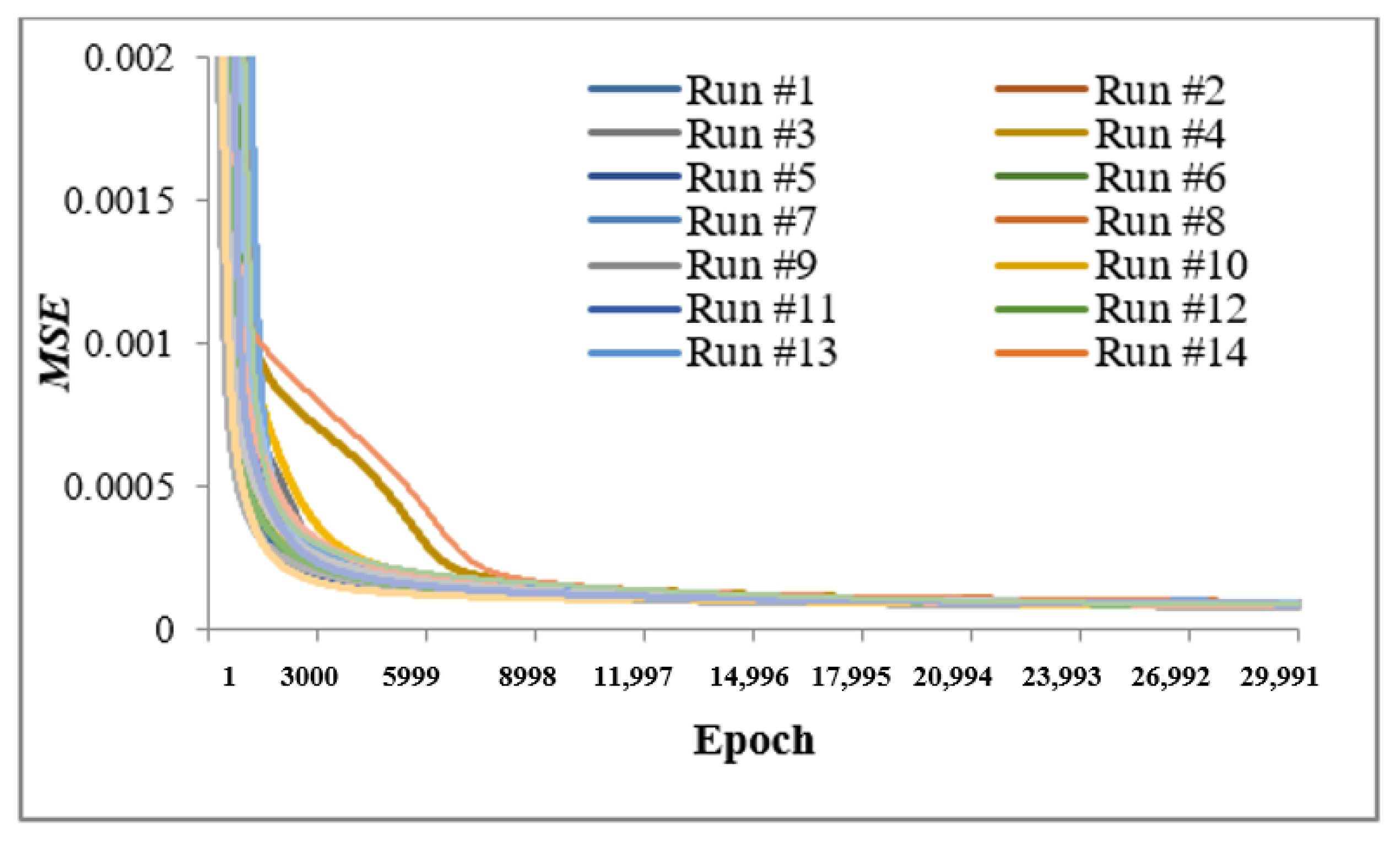
3.2. Experimental Characteristics

The research presented in this article utilizes the dataset created by Tsanas and Xifara [14]. As noted, this particular dataset has been used by other researchers that have explored the use of predictive analytics for studies within energy systems. Since various sensitivity analysis techniques are being explored in this article, it is critical that an accurate model is developed. By analyzing a dataset that has been explored by others in the research community, comparisons related to the quality-of-fit can be made in order to ensure that the model generated for this research is as accurate as what others have produced from the research community. In order to evaluate the accuracy of the proposed framework, various experiments were designed. In each experiment, 55% of the records were randomly selected for training, 15% were randomly selected for validation, and the remaining 30% of the records were held out for independent testing. Cross-validation (CV) is an important part of determining how well the model will perform when it encounters data that was not a part of training or even testing data. In other words, it is useful to see how a model generalizes data it has never seen before. Normalization, MA, and randomization are preprocessing procedures that were applied to the dataset in order to improve generalizability. The number of training runs for each model developed was set to 30, with 30,000 epochs. If the model did not experience improvements within 100 epochs for the validation data, the training routine was terminated, and the next model repeated the training process. Finding the most accurate model when it comes to the performance measures of the test records can be an arduous task. Next, statistical analysis was implemented to compare the performance of different experiments. Finally, both the local and global SA techniques were applied in order to rank the inputs according to their ability to forecast HL and CL. ANN and DNN models were developed in NeuroSolutions 7 software (NeuroSolutions, Inc., Denver, Colorado, USA). Figure 2 indicates the procedure implemented to forecast EPB.
In the experiments that were performed in this study, all of the models were developed with hyperbolic tangent neurons, which were represented in the software as TanhAxon, and momentum was used for the learning method. Since TanhAxon was used, the range of each neuron varied between −1 and 1. Equation (1) shows the calculation for a TanhAxon. In this equation, x i is the record associated with input i, w i is the weight associated with the bias vector, and x i l i n is the scaled term adapted from a Linear Axon.
f ( x i , w i ) = tanh [ x i l i n ]
The momentum leaning rule produced a value between 0 and 1, and the weight was applied within the objective function to avoid achieving a local-optimal solution. In other words, momentum helped to avoid sub-optimal results. In general, a large value for momentum translated into faster convergences and required a smaller learning rate. A small value of momentum generally decreased training time but did not guarantee optimal local results.
Table 3 shows the characteristics of the empirically designed experiments that were conducted. Empirical designs that explore machine learning methods for energy studies are commonly used by the research community. For example, Sekhar et al. [4], Alam et al. [22], Fei et al. [23], and Nwulu [28] have all used an empirical design for their design procedure. In terms of Table 3, the first experiment involved creating a single ANN that consisted of two outputs (i.e., HL and CL). This particular experiment used a single hidden layer and five processing elements. Likewise, experiments 2 and 11 were ANNs that consisted of single hidden layer network designs with five processing elements; however, unlike with experiment 1, the ANN had only one output. In order to identify the appropriate number of layers and processing elements, considerably more experiments were conducted. For example, in experiments 3 through 10, HL was forecasted with DNNs. Likewise, in experiments 12 through 19, CL was forecasted with DNNs. Moreover, in order to explore the effects of randomization and MA, additional experimental configurations were considered.
Figure 3a represents the network for experiment 1 in which HL and CL were forecasted by a single model. This type of neural network in experiment 1 used an ANN and consisted of one hidden layer with five processing elements. Figure 3b visualizes the DNN network for experiments 3 and 12, which forecasted HL and CL in separate models, respectively. Each of the models consisted of two hidden layers. The number of processing elements in the first and the second hidden layers were five and four, respectively.

3.3. Performance Measures

This section summarizes goodness-of-fit metrics which were useful in evaluating the performance of the developed models. Two main dimensions—trend fit and location fit—were important in presenting the given data. Trend fit specifies whether the displayed data captures the data trends, while location fit evaluates whether it is possible to easily evaluate the accuracy of the model by following the location of the predicted points [36]. Among the performance measures presented in this section, the coefficient of determination (R2) is representative of trend fit, while the root mean square error (RMSE), mean absolute error (MAE), prediction interval (PI), and score are representative of location fit. Low values for RMSE and MAE indicate high model accuracy. R2 values close to 1 and score values close to 100% show predicted outputs that are similar to the actual output values. PI depends upon the prediction level identified by the user.
RMSE calculates the average square error of prediction and is useful when capturing large differences between predicted and actual outputs. RMSE is calculated using the following equation:
R M S E =   ( 1 n ) × i = 1 n [ p i y i ] 2
MAE indicates the average absolute value of the magnitude of the error, and is calculated using the following equation:
M A E = 1 n ×   i = 1 n ( | p i y i | )
R2 measures the proportion of variance in the dependent variable that is predictable via the independent variables. The following equation calculates R2:
R 2 = 1 S S E S S T = 1   i = 1 n ( y i   p i ) 2 i = 1 n ( y i   y ¯ ) 2
In Equations (2) to (4), p i identifies the predicted value for sample i, y i identifies the actual value for sample i, n is the sample size, y ¯ indicates the mean of the predicted values, SSE indicates the residual sum of squares, and SST indicates the total sum of the square.
PI is designed to capture the fluctuations of the dependent variable in future observations and is calculated using the following equation:
P I = Y ^ ± t , n 2 *   s y   1 + 1 n + ( x * x ¯ ) 2 ( n 1 ) s X 2 .
where Y ^ indicates the estimated response value, t n 2 * represents the t distribution with a prediction level of 1 and n−2 degrees of freedom, n refers to the number of rows in the dataset, s y is the residual standard error in regression output, x * is the given data for an independent variable, x ¯ is the sample mean, and s X 2 is the residual standard error in regression input. This score measures the accuracy of the model based on its statistics, which include the normalized root mean squared error and the normalized mean absolute error for regression models.

4. Results

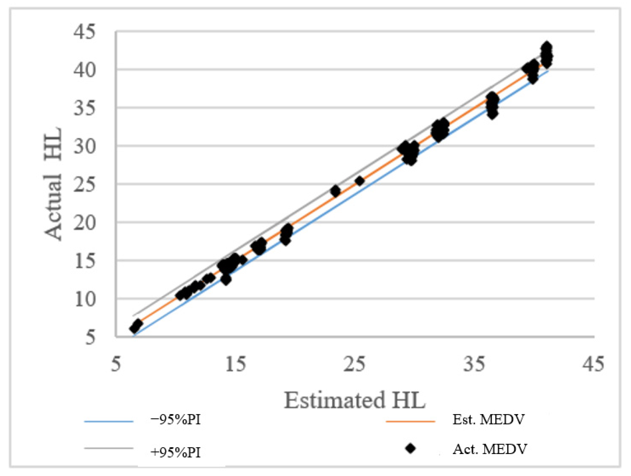
4.1. Comparison of ANN and DNN Performance

This section applies the proposed methodology and summarizes the results of the experimental procedure. The outputs of the ANN and DNN models are summarized in Table 4 for the testing dataset and in Table 5 for the training dataset. Experiments 7 to 10 and 16 to 19 adopted randomization, while experiments 20 and 21 adopted MA as data preprocessing techniques. According to Table 4 the best performance found for HL was experiment 9, and the best-performing model for CL was experiment 18. Experiments 9 and 18 consisted of three hidden layers, where the first, second, and third layers consisted of 10, 8, and 8 processing elements, respectively. Comparing the performance measures in experiments 5 and 9 indicated that, by applying randomization as a data preprocessing technique, RMSE was improved by 44.37%. The same comparison for CL shows an improvement of 50.07% in RMSE. Applying MA as a data preprocessing technique improved RMSE for HL by 16.34%; however, it did not improve the performance measures of CL. Different periods of MA were tested, and the results of the best MA period equaled 5. As noted, the first experiment forecasted HL and CL as outputs in a single ANN model. Comparing the results of experiment 1 with experiment 2 shows that, when HL and CL were forecasted in a single model, the accuracy of HL was 26.51% higher than if we were to consider HL in a separate model; however, comparing experiments 1 and 11 showed that the same conclusion was not applicable for CL since RMSE in experiment 11 was improved by 14.95%. Models using DNNs significantly increased forecasting accuracy. For example, comparing the results of experiment 2 (in which an ANN was applied) to experiment 3 (in which a DNN was applied) yielded an improvement of 28.69% in RMSE when it came to forecasting HL. Comparing the results of experiment 11 to experiment 12 showed that, by adding an additional hidden layer, RMSE for CL forecasting improved by 14.47%.
Table 5 shows the results of the experiments with respect to the training dataset. The best-performing model was associated with experiment 10 when it came to forecasting HL and experiment 18 when it came to forecasting CL. Applying MA improved the forecasting accuracy of HL by 7.18% and the forecasting accuracy of CL by 6.63%. Analysis of the improvements in the performance measurements of these training records showed the same results obtained from the testing records. More specifically, separating HL and CL into individual models improved the forecasting performance of CL, but decreased the accuracy in forecasting HL. However, in both cases of HL and CL prediction, the DNN models showed an improvement over the ANN models. In addition, randomization and MA also improved the forecasting of HL and CL.
Figure 4 shows the learning curve associated with experiment 9, which represents the highest-performing model for HL. The learning curve plots the square difference between the actual values and the network output (MSE) as a function of time measured as an epoch. During the training phase, the network learned from the training records while the error decreased and reached zero exponentially. The stopping criteria are important factors when training an ANN or DNN. For example, training was terminated when MSE performance did not improve by a predetermined amount over a defined number of iterations. In experiment 9, the best training network was obtained in run 21 at 30,000 epochs.
Table 6 and Table 7summarize the performance measures of HL and CL in training and testing results, respectively. The results found in recent literature were compared with the results obtained from the research conducted and presented in this article. One observation that was made while reviewing the literature was that some of the previous research conducted did not consider cross-validation; therefore, as a result, it is possible that some of these models might exhibit over-fitting. Table 6 and Table 7 summarize these studies by stating the goodness-of-fit statistics that were reported in the related studies. Moreover, the normalized or non-normalized values of MSE and RMSE were reported, depending upon the availability of the information presented in the literature published at the time of this investigation. Thus, some of the information appears to be incomplete; however, this is simply due to the fact that not all of the information was reported.
In order to obtain additional insight into the performance of the proposed model, prediction intervals for experiment 9 were constructed. Figure 5 shows the 95% prediction intervals for experiment 9, which obtained the highest forecasting accuracy among HL models in the experiments conducted with respect to the testing data. As Figure 5 indicates, there are six observations that fall outside of the prediction intervals. This proportion is 6.96%, which is close to the theoretical value of 5% (with the associated 95% prediction level).

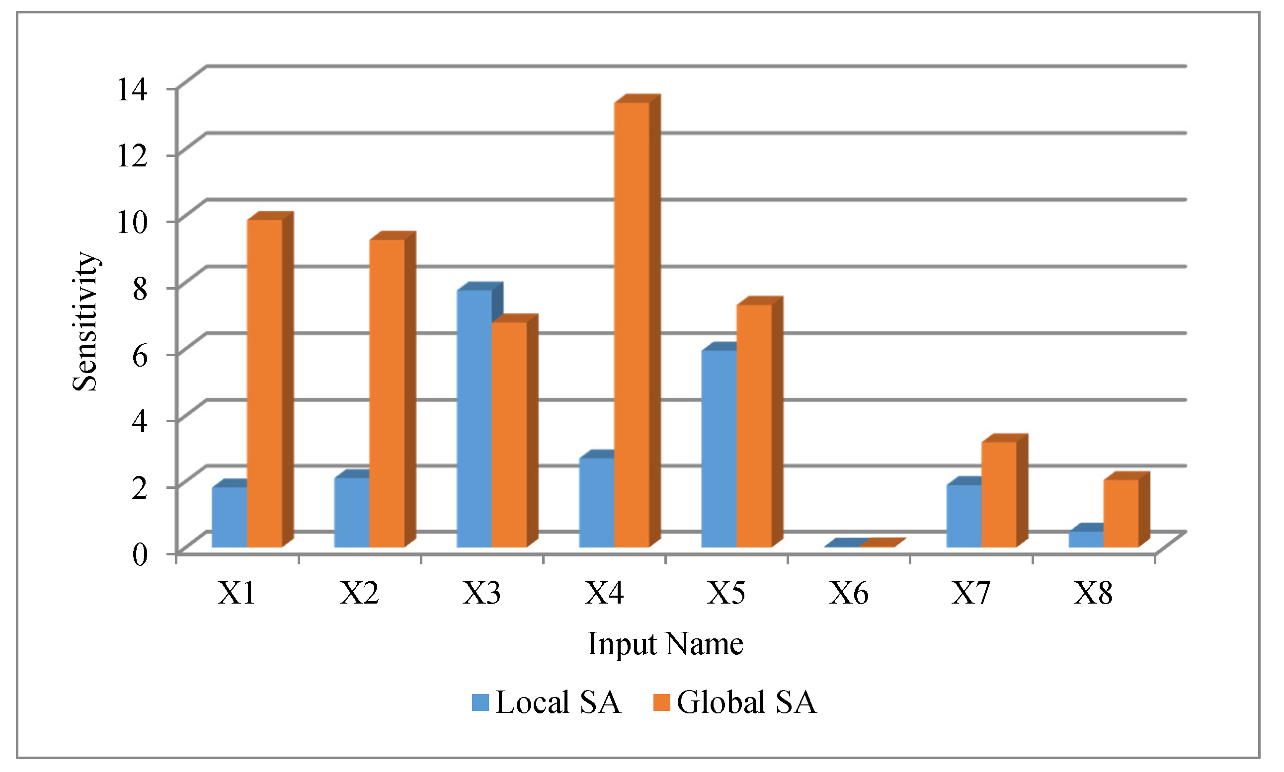
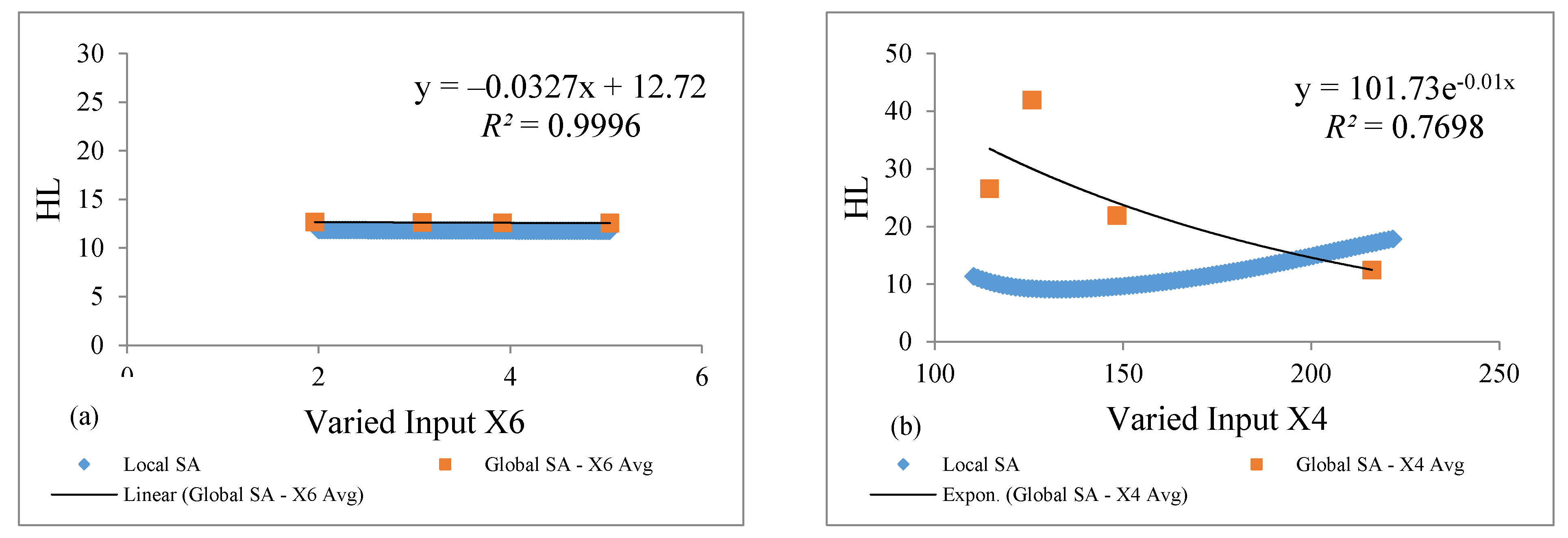
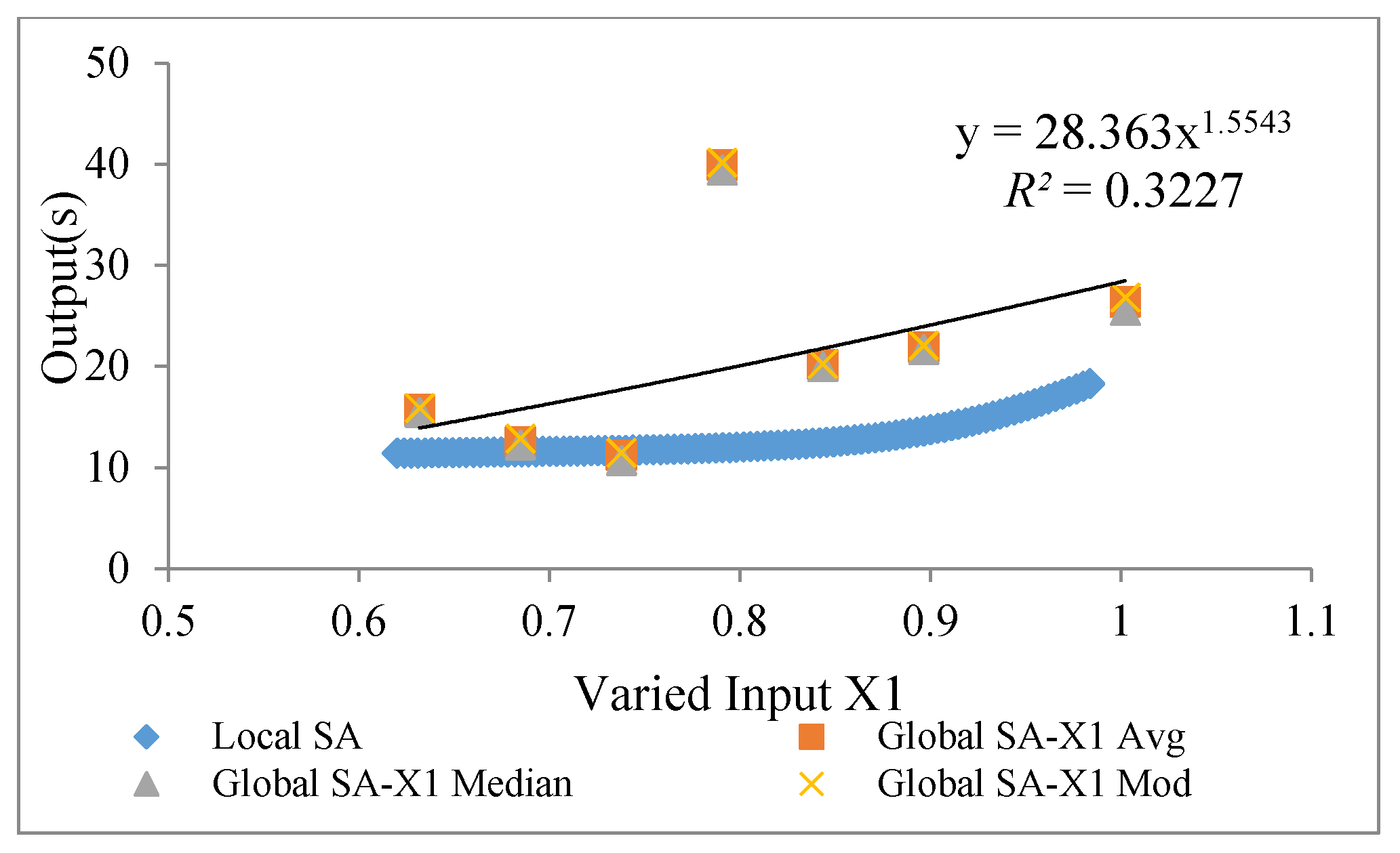
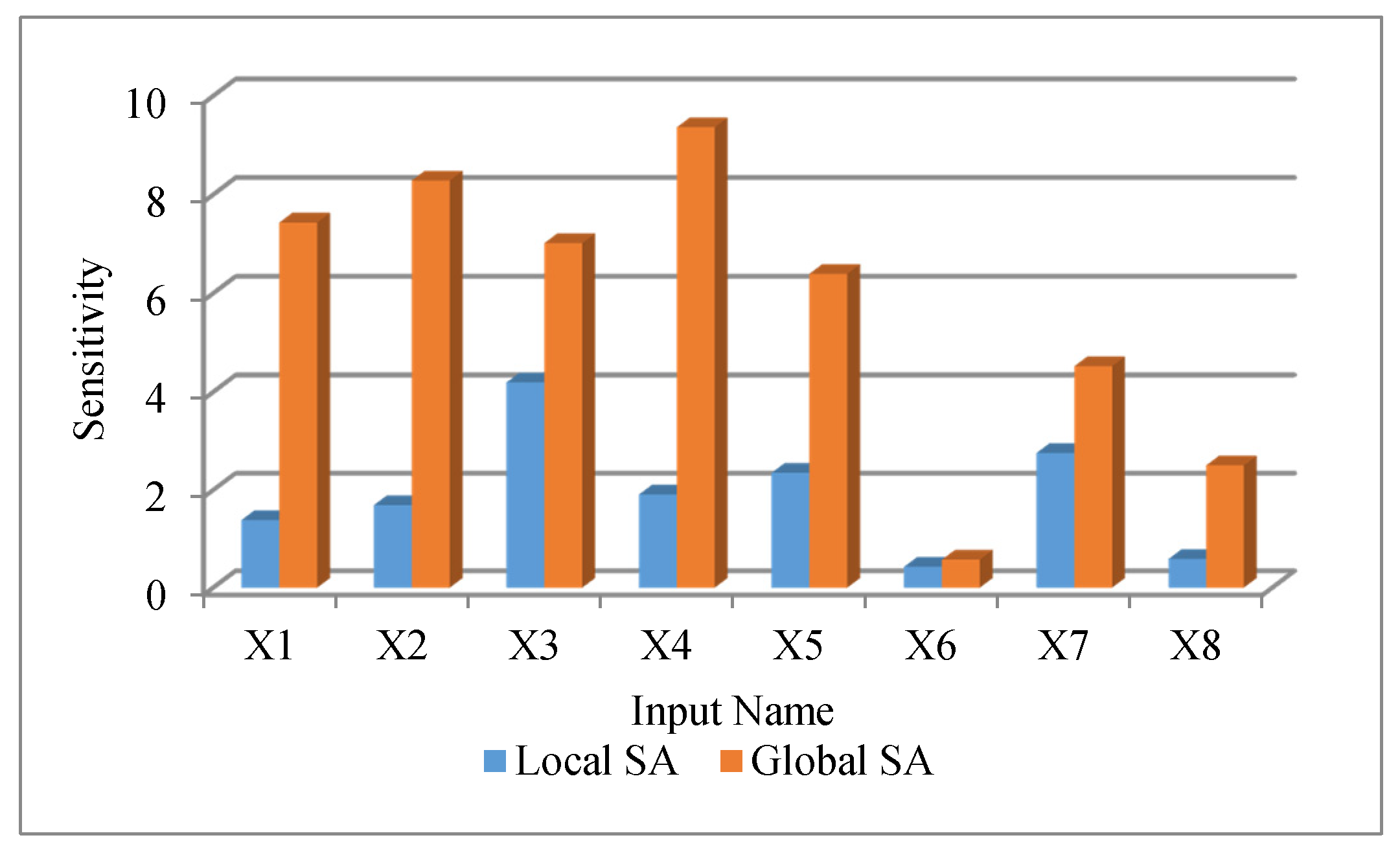
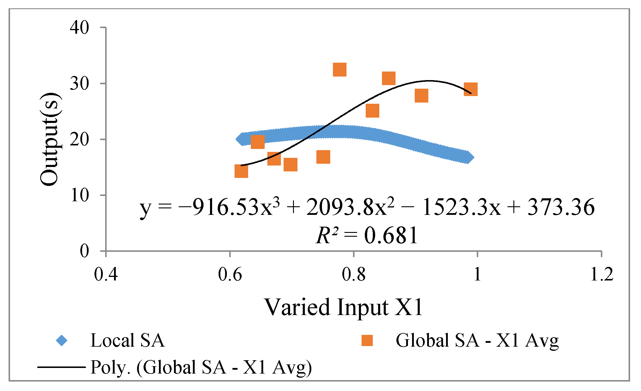
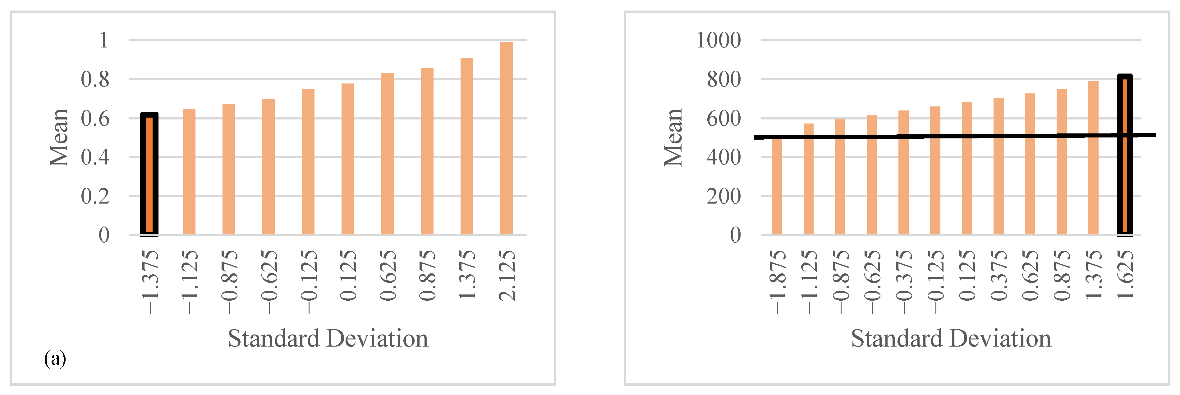
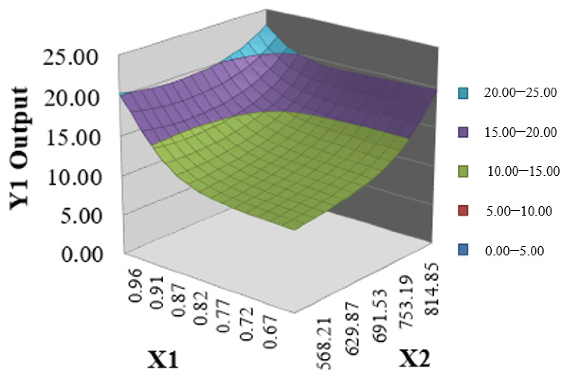
4.2. Local and Global SA

The objective of this section is to apply SA in order to determine how variations in the output variables can be explained by variations in the input parameters. Both SAAM and SBSA attempt to capture the relationships between dependent and independent variables. SAAM is an automated process and is also a feature available in NeuroSolutions 7. Using this technique, one variable is changed at a time, and the difference in output is recorded. Each variable is changed over a range of 50 step sizes with a range of ±3 standard deviation of the attribute’s mean, while all other variables are held at their sample mean. SAAM examines the influence of each attribute independent from the other attributes. However, local SAAM ignores the lack of multicollinearity among database variables. Independence among multiple input variables is typically not a valid assumption and reduces the ability to accurately predict a response variable. For example, if two variables are highly correlated, analyzing the model’s predictive ability for a given variable while keeping the value of the other variable static (as an average), is neither appropriate nor logical. The assumption of independence and non-association between these two inputs is incorrect.
On the other hand, SBSA incorporates the presence of the multivariate relationships amongst all the variables. For example, the value of all variables changes when just one input attribute is varied. For each variable, a few intervals are defined with respect to the mean and standard deviation of the sample population. These intervals were assigned to a “state” (± standard deviation value). The range wherein every “state” was equivalent to a predetermined standard deviation of that distribution. This allowed the predictor influences to represent themselves as input probability density functions by averaging the correlations among multiple inputs. Table 8 indicates the correlation matrix for the studied problem. For example, X2 has a negative correlation to Y1 and Y2, while X5 has a positive correlation.
Adjusting both predictor variables to their respective states allows for a calculation of the overall effects that more accurately determines the output variable. The higher the standard deviation, the more important an input attribute is to a model. This implies that small changes for a sensitive attribute result in large changes to the output variable. Likewise, an insensitive attribute implies that large changes of an input can be made with very little effect on the output of a model. This is the main advantage of global over local (SAAM) methods. Ardjmand et al. [9] provided a detailed analysis of SBSA. Figure 6 shows the result of applying SAAM and SBSA for experiment 9, where the Y-axis shows the standard deviation of HL with respect to each of the inputs which are shown along the X-axis.
As Figure 6 indicates, both SAAM and SBSA show that the least significant input is X6 (orientation) for HL. The low influence of X6 is also expected according to the associated correlation in Table 8. SAAM shows X3 (wall area) is the most significant input for HL, while SBSA shows that the most significant attribute for HL is X4 (roof area). Though Figure 6 is useful in determining which input attribute is the most and least sensitive, it does not show how the output variable changes with respect to changes in input. In Figure 7, the change of HL is shown as a function of X4 and X6 for both the SAAM and the SBSA techniques. Figure 7a shows that the orientation of the building (X6) is insignificant since changing the value of the orientation from −3 to +3 standard deviation does not change the output of HL. This result is consistent in both the SAAM and SBSA. However, the results in Figure 7b show that the SAAM and SBSA produce different behaviors in terms of how the output reacts to a change in X4. In other words, SAAM suggests that increasing the roof area (X4) requires more heat within the building when the building is cold (HL). However, the SBSA suggests that increasing the roof area (X4) ultimately requires less HL within buildings.
At first glance, the idea that as roof area increases, the HL would have a lower requirement may not seem intuitive, but let us look at the interaction of 2 variables with respect to HL. First, as the roof area increases, the ratio of the outside exposure with the exterior wall area decreases. The exterior wall area has a smaller impact on the overall energy requirements (cold outside temperatures) due to this lower ratio of square footage exposure to the total area being heated. This is mainly because exterior walls (typically those with windows) have a much higher energy loss transfer compared to roofs [37]. This is confirmed by an analysis completed by Agarwal [38] on the current dataset, in which the relationship between roof areas and heating and cooling loads is discussed.
Figure 8 shows the results of SAAM and SBSA associated with X1 (relative compactness). The figure shows that the distribution of change is unimodal since the values of mean, mode, and median are approximately the same for each of the seven different state values. The value of R2 shows a low accuracy in terms of the trend found with SBSA. Both SAAM and SBSA represent a continuous increase in HL when relative compactness increases. However, SBSA shows a more dramatic increase in HL when the relative compactness changes. Notice that in the correlation shown in Table 8, the correlation of X1 was very positive with respect to HL (Y1), which supports the SBSA relationship.
Figure 9 shows the variation of CL after applying SAAM and SBSA for experiment 18. Similar insights that were obtained for HL (in regards to the significance of the input variables) are also applicable for CL. For example, both SAAM and SBSA show that the least significant input is X6 (orientation). However, in terms of the most significant input attribute for CL, the results are inconsistent. For example, SAAM suggests that X3 (wall area) is the most significant input, while SBSA suggests that X4 (roof area) is the most significant input. As discussed previously, the literature supports the fact that the roof area typically has more of an impact than the wall area. In addition, the correlation for X4 is twice as much as X3 regarding both CL and HL.
Figure 10 shows the behavior of CL when changing X1 (relative compactness). SAAM suggests that, by increasing the relative compactness, CL remains fairly stable until, at one point, the value of CL gradually decreases. This is much different than the results of SBSA. For example, the SBSA technique suggests that, for the most part, a constant increase of CL is obtained when the relative compactness increases. It should be noted that Figure 8 shows that SAAM and SBSA both suggest that increasing the relative compactness also results in an increase in the value of HL. Sharizatul et al. [39] reinforce this relationship in which the more compact the form of a building, the lower the cooling load will be. Another interesting observation regarding relative compactness (X1) in this study is the step increase after a value of about 0.75. It seems there are two different clusters of buildings. Figure 11 supports this observation since all relative compactness above 0.75 are two-story buildings. All of the two-story buildings will have considerably higher ratios of wall-area-to-roof-area, which will result in higher HL and CL.
Readers of this article might be asking which SA should be trusted or is more accurate. This, of course, is a difficult question to answer. However, the evidence would suggest that SBSA represents true system dynamics more accurately. For example, Figure 11a shows that X1 consists of 10 states. This figure also shows the mean of each state for the X1 variable. Likewise, Figure 11b shows that X2 also has 10 states, and the respective mean for each state is also shown. State graphs like the ones shown in Figure 11 help us to understand what one input attribute’s value is likely to be when another variable is a certain value. For example, when X1 is at its lowest state value (highlighted in Figure 11a), X2 is likely to be at its highest state value, which is highlighted in Figure 11b. This means that when X1’s value is around 0.6, it is likely that X2’s value will be around 800. Furthermore, state graphs like the ones presented below provide evidence that SAAM, although a popular technique, fails to capture the true multivariate nature of complex system dynamics. For example, the average value of X2 is just above 600. In SAAM, the average value for X2 (approximately 600) would be used for all value ranges in X1 (approximately 0.6 to 1.0). As shown in Figure 11, this is not the case and will build inaccuracies when estimating the value of the output variable. SBSA suggests that while X1 is valued at around 0.6, the value of X2 should be much higher, at around 800.
Though two-dimensional (2D) plots are useful when it comes to understanding the underlying behavior of the data being modeled, a deeper analysis can be conducted. Figure 12 shows a three-dimensional (3D) relationship between X1 (relative compactness), X2 (surface area), and the model’s forecasted value of HL, given that SBSA is employed. Based on this analysis, the relationships that occur when X1 and X2 are varied simultaneously can be more easily understood. For example, as X1 and X2 both decrease, so does the value of HL. Likewise, higher values of HL are the result of high values of both X1 and X2. From a design perspective, the three-dimensional SBSA could help building designers achieve more desirable building characteristics. For example, if a minimum value of HL is desired, this can be obtained by minimizing both X1 (relative compactness) and X2 (surface area). The problem with this relationship is that the correlation between X1 and X2 have opposite impacts on HL and CL. In this scenario, some of the areas on the graph will not be achievable. This 3D graph can be fitted to an equation, and then the designer can vary characteristics of the building in order to optimize the HL and CL (while still keeping in mind other factors).

5. Conclusions

Residential buildings consume a considerable proportion of total energy consumption, which results in environmental pollution. This paper evaluated the application of both machine-learning and deep-learning techniques in order to forecast the HL and CL of the residential buildings for a specific dataset. Comparing the results of ANNs and DNNs showed that DNNs outperform ANNs in terms of forecasting accuracy for HL and CL. Therefore, the results of this study support the application of deep learning in the area of EPB. Though the experimental design focused on within this research suggests that forecasting HL and CL in a combined or separated manner results in different predictive accuracies, by adding an MA component as a preprocessing step, the quality of the models improved. In addition to this step, the data used in this investigation was also normalized and randomized into training, testing, and cross-validation data partitions. These simple yet effective steps were shown to improve predictive capabilities when comparing the best model found in this study to other reported models in the literature. Additional statistical analysis was performed on the models that performed the best on independent testing data. This analysis included the development of a 95% prediction interval, which gives practitioners additional information in terms of how well the model generalized the dynamics within the mined data. The study presented in this article applied SAAM, which is a local SA, as well as a global SA called SBSA. These techniques were invoked in order to analyze the impact of each independent variable. In addition, these methods were compared and contrasted with a few variables of interest. SA provided insight as to the effect each input had on predicting HL and CL. In some cases, the analysis showed conflicting results. However, when certain input variables can be correlated with certain other input variables, global sensitivity methods like SBSA provide more realistic results than local SA approaches like SAAM. From a data-mining perspective, identifying and eliminating less significant inputs can decrease the overall complexity of the system being modeled, as well as lessen the time needed to develop a machine-learning method such as DNNs. By knowing the most sensitive variables of a model, it is possible to leverage that model from a design standpoint, especially in the field of EPB.

Author Contributions

Conceptualization, W.A.Y.II and G.R.W.; Formal analysis, A.S., R.Y.S., W.A.Y.II and G.R.W.; Funding acquisition, G.R.W.; Investigation, A.S., R.Y.S., W.A.Y.II and G.R.W.; Methodology, A.S., R.Y.S., W.A.Y.II and G.R.W.; Project administration, W.A.Y.II and G.R.W.; Supervision, W.A.Y.II and G.R.W.; Validation, A.S., R.Y.S., W.A.Y.II and G.R.W.; Visualization, A.S., R.Y.S., W.A.Y.II and G.R.W.; Writing—original draft, A.S. and R.Y.S.; Writing—review & editing, A.S., R.Y.S., W.A.Y.II and G.R.W. All authors have read and agreed to the published version of the manuscript.

Funding

This research received no external funding.

Conflicts of Interest

The authors declare no conflict of interest.

Nomenclature

AbbreviationDescriptionAbbreviationDescription
EMARSEvolutionary Multivariate Adaptive Regression SplinesOLSOrdinary Least Squares
MARSMultivariate Adaptive Regression SplinesPLSPartial Least Squares
MIMutual InformationGPRGaussian Process Regression
IRLSIteratively Reweighted Least SquaresMPMRMinimax Probability Machine Regression
RFRandom ForestMAEMean Absolute Error
DTDecision TreeRMAERoot Mean Absolute Error
SVRSupport Vector MachineMAPEMean Absolute Percentage Error
ABC-KNNArtificial Bee Colony-Based K-Nearest NeighborWMAPEWeighted Mean Absolute Percentage Error
GA-KNNGenetic Algorithm-Based K-Nearest NeighborMSEMean Square Error
GA-ANNAdaptive Artificial Neural Network with Genetic AlgorithmRMSERoot Mean Square Error
ABC-ANNAdaptive ANN with Artificial Bee ColonyR2Coefficient of Determination
SVRSupport Vector RegressionVAFVariance Accounted For
ANOVAAnalysis of VarianceRAAERelative Average Absolute Error
ANFISAdaptive Neuro-Fuzzy Inference SystemNSNash-Sutcliffe
ELMExtreme Learning MachineMREMean Relative Error
SDStandard DeviationrPearson Correlation Coefficient
SISynthesis IndexRRSERoot Relative Square Error
EMExpected MaximizationRAERelative Absolute Error
PCAPrincipal Component Analysis

References

  1. International Energy Agency (IEA). Transition to Sustainable Buildings; International Energy Agency (IEA): Paris, France, 2013; ISBN 978-92-64-20241-2. [Google Scholar]
  2. International Energy Agency (IEA). Energy Efficiency: Buildings; International Energy Agency (IEA): Paris, France, 2018. [Google Scholar]
  3. Roy, S.S.; Roy, R.; Balas, V.E. Estimating heating load in buildings using multivariate adaptive regression splines, extreme learning machine, a hybrid model of MARS and ELM. Renew. Sustain. Energy Rev. 2018, 82, 4256–4268. [Google Scholar]
  4. Sekhar, S.; Pijush, R.; Ishan, S.; Hemant, N.; Vishal, J. Forecasting heating and cooling loads of buildings: A comparative performance analysis. J. Ambient Intell. Humaniz. Comput. 2019, 1–12. [Google Scholar] [CrossRef]
  5. Bouktif, S.; Fiaz, A.; Ouni, A.; Serhani, M. Optimal Deep Learning LSTM Model for Electric Load Forecasting using Feature Selection and Genetic Algorithm: Comparison with Machine Learning Approaches. Energies 2018, 11, 1636. [Google Scholar] [CrossRef] [Green Version]
  6. Yu, W.; Li, B.; Lei, Y.; Liu, M. Analysis of a Residential Building Energy Consumption Demand Model. Energies 2011, 4, 475–487. [Google Scholar] [CrossRef]
  7. Seyedzadeh, S.; Rahimian, F.P.; Glesk, I.; Roper, M. Machine learning for estimation of building energy consumption and performance: A review. Vis. Eng. 2018, 6, 5. [Google Scholar] [CrossRef]
  8. Bagheri, A.; Feldheim, V.; Ioakimidis, C. On the Evolution and Application of the Thermal Network Method for Energy Assessments in Buildings. Energies 2018, 11, 890. [Google Scholar] [CrossRef] [Green Version]
  9. Ardjmand, E.; Millie, D.F.; Ghalehkhondabi, I.; Ii, W.A.Y.; Weckman, G.R. A State-Based Sensitivity Analysis for Distinguishing the Global Importance of Predictor Variables in Artificial Neural Networks. Adv. Artif. Neural Syst. 2016, 2016, 2303181. [Google Scholar] [CrossRef] [Green Version]
  10. Weckman, G.R.; Millie, D.F.; Ganduri, C.; Rangwala, M.; Young, W.; Rinder, M.; Fahnenstiel, G.L. Knowledge Extraction from the Neural ‘Black Box’ in Ecological Monitoring Knowledge Extraction from the Neural ‘Black Box’ in Ecological Monitoring. Int. J. Ind. Syst. Eng. 2009, 3, 38–55. [Google Scholar]
  11. Millie, D.F.; Weckman, G.R.; Young, W.A.; Ivey, J.E.; Carrick, H.J.; Fahnenstiel, G.L. Environmental Modelling & Software Modeling microalgal abundance with artificial neural networks: Demonstration of a heuristic ‘Grey-Box’ to deconvolve and quantify environmental influences. Environ. Model. Softw. 2012, 38, 27–39. [Google Scholar]
  12. Saltelli, A.; Tarantola, S.; Campolongo, F.; Ratto, M. Sensitivity Analysis in Practice: A Guide to Assessing Scientific Models; Wiley: Chichester, UK, 2004. [Google Scholar]
  13. Yeung, D.S.; Cloete, I.; Shi, D.; Ng, W.W.Y. Sensitivity Analysis for Neural Networks; Springer: Berlin/Heidelberg, Germany, 2010. [Google Scholar]
  14. Tsanas, A.; Xifara, A. Accurate quantitative estimation of energy performance of residential buildings using statistical machine learning tools. Energy Build. 2012, 49, 560–567. [Google Scholar] [CrossRef]
  15. Yezioro, A.; Dong, B.; Leite, F. An applied artificial intelligence approach towards assessing building performance simulation tools. Energy Build. 2008, 40, 612–620. [Google Scholar] [CrossRef]
  16. Bourdeau, M.; Nefzaoui, E.; Guo, X.; Chatellier, P. Modeling and forecasting building energy consumption: A review of data-driven techniques. Sustain. Cities Soc. 2019, 48, 101533. [Google Scholar] [CrossRef]
  17. Park, S.; Ryu, S.; Choi, Y.; Kim, J.; Kim, H. Data-Driven Baseline Estimation of Residential Buildings for Demand Response. Energies 2015, 8, 10239–10259. [Google Scholar] [CrossRef] [Green Version]
  18. Chou, J.; Bui, D. Modeling heating and cooling loads by artificial intelligence for energy-efficient building design. Energy Build. 2014, 82, 437–446. [Google Scholar] [CrossRef]
  19. Cheng, M.; Cao, M. Accurately predicting building energy performance using evolutionary multivariate adaptive regression splines. Appl. Soft Comput. J. 2014, 22, 178–188. [Google Scholar] [CrossRef]
  20. Ahmed, A.; Srihari, K.; Khasawneh, M.T. Integrating Artificial Neural Networks and Cluster Analysis to Assess Energy Efficiency of Buildings. In Proceedings of the 2014 Industrial and Systems Engineering Research Conference, Montreal, QC, Canada, 31 May–3 June 2014. [Google Scholar]
  21. Sonmez, Y.; Guvenc, U.; Kahraman, H.T.; Yilmaz, C. A Comperative Study on Novel Machine Learning Algorithms for Estimation of Energy Performance of Residential Buildings. In Proceedings of the 2015 3rd International Istanbul Smart Grid Congress and Fair (ICSG), Istanbul, Turkey, 29–30 April 2015; pp. 1–7. [Google Scholar]
  22. Alam, A.G.; Baek, C.; Han, H. Prediction and Analysis of Building Energy Efficiency Using Artificial Neural Network and Design of Experiments Prediction and Analysis of Building Energy Efficiency using Artificial Neural Network and Design of Experiments. Appl. Mech. Mater. 2016, 819, 541–545. [Google Scholar]
  23. Fei, Y.; Pengdong, G.; Yongquan, L. Evolving Resilient Back-Propagation Algorithm for Energy Efficiency. MATEC Web Conf. 2016, 77, 06016. [Google Scholar]
  24. Regina, G.; Capriles, P. Prediction of energy load of buildings using machine learning methods database and machine learnig methods. In Proceedings of the Conference of Computational Interdisciplinary Science, São José dos Campos, Barzil, 7–10 November 2016. [Google Scholar]
  25. Naji, S.; Shamshirband, S.; Basser, H.; Keivani, A. Application of adaptive neuro-fuzzy methodology for estimating building energy consumption. Renew. Sustain. Energy Rev. 2016, 53, 1520–1528. [Google Scholar] [CrossRef]
  26. Naji, S.; Keivani, A.; Shamshirband, S.; Alengaram, U.J.; Zamin, M.; Lee, M. Estimating building energy consumption using extreme learning machine method. Energy 2016, 97, 506–516. [Google Scholar] [CrossRef]
  27. Nilashi, M.; Dalvi-esfahani, M.; Ibrahim, O.; Bagherifard, K. A soft computing method for the prediction of energy performance of residential buildings. Measurement 2017, 109, 268–280. [Google Scholar] [CrossRef]
  28. Nwulu, N.I. An artificial neural network model for predicting building heating and cooling loads. In Proceedings of the 2017 International Artificial Intelligence and Data Processing Symposium (IDAP), Malatya, Turkey, 16–17 September 2017; pp. 0–4. [Google Scholar]
  29. Duarte, G.R.; Vanessa, P.; Capriles, Z.; Celso, A.; Lemonge, D.C. Comparison of machine learning techniques for predicting energy loads in buildings. mbiente Construído 2017, 17, 103–115. [Google Scholar] [CrossRef] [Green Version]
  30. Kavaklioglu, K. Robust modeling of heating and cooling loads using partial least squares towards efficient residential building design. J. Build. Eng. 2018, 18, 467–475. [Google Scholar] [CrossRef]
  31. Kumar, S.; Pal, S.K.; Pal, R. Intra ELM variants ensemble based model to predict energy performance in residential buildings. Sustain. Energy Grids Netw. 2018, 16, 177–187. [Google Scholar] [CrossRef]
  32. Al-Rakhami, M.; Gumaei, A.; Alsanad, A.; Alamri, A.; Hassan, M.M. An Ensemble Learning Approach for Accurate Energy Load Prediction in Residential Buildings. IEEE Access 2019, 7, 48328–48338. [Google Scholar] [CrossRef]
  33. Cariboni, J.; Gatelli, D.; Liska, R.; Saltelli, A. The role of sensitivity analysis in ecological modelling. Ecol. Modell. 2006, 3, 167–182. [Google Scholar] [CrossRef]
  34. Saltelli, A.; Ratto, M.; Andres, T.; Campolongo, F.; Cariboni, J.; Saisana, M. Global Sensitivity Analysis: The Primer; John Wiley & Sons: Hoboken, NJ, USA, 2008. [Google Scholar]
  35. Bache, M.L.K. UCI Machine Learning Repository; University of California: Irvine, CA, USA, 2012. [Google Scholar]
  36. Schunn, C.D.; Wallach, D. Evaluating Goodness-of-Fit in Comparison of Models to Data. Psychol. Kognit. Reden Vor. Anlässlich Emeritierung Werner Tack 2005, 1, 115–135. [Google Scholar]
  37. Geletka, V.; Sedlákováa, A. Shape of buildings and energy consumption. Czas. Tech. Bud. 2012, 109, 124–129. [Google Scholar]
  38. Saxena, A.; Agarwal, N.; Srivastava, G. Energy savings parameters in households of Uttar Pradesh, India. TERI Inf. Dig. Energy Environ. 2012, 11, 179–188. [Google Scholar]
  39. Sharizatul, W.; Rashdi, S.W.M.; Embi, M.R. Analysing Optimum Building Form in Relation to Lower Cooling Load. Procedia Soc. Behav. Sci. 2016, 222, 782–790. [Google Scholar]
Figure 1. Training Records: (a) Actual output of heating load (HL) and cooling load (CL); (b) Randomized output of HL and CL; (c) Scatter plot.
Energies 13 00571 g001
Figure 2. Methodology Framework.
Energies 13 00571 g002
Figure 3. Graphical Representation of the Proposed DNN for (a) Experiments 1 and (b) Experiment 3 and 12.
Energies 13 00571 g003
Figure 4. Learning curve: Experiment 9.
Energies 13 00571 g004
Figure 5. Prediction interval (PI) for testing data: Experiment 9.
Energies 13 00571 g005
Figure 6. Comparison of local and global sensitivity for Heating Load (HL).
Energies 13 00571 g006
Figure 7. Network output (HL) for varied (a) orientation (X6) and (b) roof area (X4).
Energies 13 00571 g007
Figure 8. Network output (HL) for varied relative compactness (X1).
Energies 13 00571 g008
Figure 9. Comparison of local and global sensitivity for HL.
Energies 13 00571 g009
Figure 10. Network output (CL) for varied relative compactness (X1).
Energies 13 00571 g010
Figure 11. (a) Different states of relative compactness (X1); (b) different states of surface area (X2).
Energies 13 00571 g011
Figure 12. Three-dimensional (3D) modeling of relative compactness (X1), surface area (X2), and HL.
Energies 13 00571 g012
Table 1. Literature Review.
Related StudiesMachine Learning MethodVariable Importance MethodCombined Outputs Evaluation Criteria
Tsanas and Xifara [14] IRLS, RFSpearman rank correlation coefficient and p-value, MI-MAE, MSE, MRE
Chou and Bui [18] Ensemble approach (SVR + ANN), SVR--RMSE, MAE, MAPE, R, SI
Cheng and Cao [19] EMARSMARS-RMSE, MAPE, MAE, R2
Ahmed et al. [20] ANN and cluster analysis-Silhouette Score
Sonmez et al. [21] ABC-KNN
GA-KNN
GA-ANN
ABC-ANN
--MAE, SD
Alam et al. [22] ANNANOVA-RMSE
Fei et al. [23] ANN--MSE
Regina and Capriles [24] DT, MLP, RF, SVR--MAE,
RMSE,
MRE,
R2
Naji et al. [25]ANFIS--RMSE, r, R2
Naji et al. [26]ELM-RMSE, r, R2
Nilashi et al. [27] EM, PCA, ANFISPCA-MAE, MAPE, RMSE
Nwulu [28] ANN--RMSE, RRSE, MAE, RAE, R2
Duarte et al. [29] DT, MLP, RF, SVM--MAE, RMSE, MAPE, R2
Roy et al. [3] multivariate adaptive regression splines, ELM, a hybrid model of MARS and ELMMARS-RMSE, MAPE, MAE, R2, WMAPE, Time
Kavaklioglu [30] OLS, PLS--RMSE, R2, Goodness of fit
Kumar et al. [31] ELM, Online Sequential ELM, Bidirectional ELM--MAE, RMSE
Al-Rakhami et al. [32] Ensemble Learning using XG Boost--RMSE, R2, MAE, MAPE
Sekhar et al. [4] DNN, GRP, MPMR--VAF, RAAE, RMAE, R2, MAPE, NS, RMSE, WMAPE
Table 2. Description of the energy performance buildings (EPB) dataset.
Variable TypeDescriptionParameters#Possible ValuesType of ParameterUnitsMinMaxAverage
Input VariablesRelative Compactness(X1)12RealNone0.620.980.76
Surface Area(X2)12Realm2514.50808.50671.71
Wall Area(X3)7Realm2245.00416.50318.50
Roof Area(X4)4Realm2110.25220.50176.60
Overall Height(X5)2RealM3.507.005.25
Orientation(X6)4IntegerNone253.50
Glazing Area(X7)4RealNone00.400.23
Glazing Area Distribution(X8)6IntegerNone052.81
Output VariablesHeating Load(Y1)586RealkWh/m26.0143.1022.31
Cooling Load(Y2)636RealkWh/m210.9048.0324.59
Table 3. Characteristics of experimental models. “PEs” stand for processing elements
ExperimentOutputHidden LayerPEs per LayerRandomization MA Neural Network
1HL and CL15--ANN
2HL15--ANN
3HL25,4--DNN
4HL35,4,4--DNN
5HL310,8,8--DNN
6HL410,8,8,8--DNN
7HL25,4-DNN
8HL35,4,4-DNN
9HL310,8,8-DNN
10HL330,24,24-DNN
11CL15--ANN
12CL25,4--DNN
13CL35,4,4--DNN
14CL310,8,8--DNN
15CL410,8,8,8--DNN
16CL25,4-DNN
17CL35,4,4-DNN
18CL310,8,8-DNN
19CL330,24,24-DNN
20HL310,8,8DNN
21CL310,8,8DNN
Table 4. Testing Results.
Exp.OutputNeural NetworkRMSE (kW)MAE (kW)R2Score (%)
1HL and CLANN(1.9269, 2.3491)(1.6850, 2.0527)(0.9906, 0.9535)(96.3351, 95.0842)
2HLANN2.43781.96110.989295.9005
3HLDNN1.73841.53780.993096.5646
4HLDNN1.86531.47830.989296.3879
5HLDNN1.20791.03050.991897.0908
6HLDNN2.22091.85760.977795.7743
7HLDNN0.71160.58460.995897.8955
8HLDNN1.02170.76940.991297.3968
9HLDNN0.67190.48280.996097.9669
10HLDNN0.92610.663410.993697.5763
11CLANN1.9981.54610.964995.7065
12CLDNN1.70881.17850.964796.0625
13CLDNN3.0092.02880.911493.6079
14CLDNN2.1171.54390.967195.6793
15CLDNN2.22321.68710.966395.5631
16CLDNN1.68081.15720.970496.2431
17CLDNN1.74661.18090.966796.0941
18CLDNN1.0570.76440.988097.2973
19CLDNN1.54611.02510.977396.5457
20HLDNN0.56210.40120.998797.9999
21CLDNN1.39291.06960.985996.8377
Table 5. Training Results.
ExperimentOutputNeural Network TypeRMSE (kW)MAE (kW)R2Score (%)
1HL and CLANN(0.7070, 1.8612)(0.5486, 1.3954)(0.9946, 0.9590)(97.8051, 95.6846)
2HLANN0.97520.74530.989697.3294
3HLDNN0.50880.36920.997298.1863
4HLDNN0.75350.57070.993997.7245
5HLDNN0.4080.29470.998298.3921
6HLDNN0.51180.32940.997298.1916
7HLDNN0.40550.30500.998098.4461
8HLDNN0.48250.36000.997498.2921
9HLDNN0.37860.2850.998498.5026
10HLDNN0.26330.20010.999998.8582
11CLANN1.56871.09360.970896.2696
12CLDNN1.61401.09930.972096.3331
13CLDNN3.22812.54040.888992.8027
14CLDNN1.62891.13130.968696.1579
15CLDNN1.59311.06040.970096.2362
16CLDNN1.61491.11650.970896.3094
17CLDNN1.581.065030.972496.3901
18CLDNN0.73860.56010.993697.8248
19CLDNN1.03590.71510.991697.4158
20HLDNN0.35140.24910.998798.5635
21CLDNN0.68960.48460.994497.8871
Table 6. Comparison of performance measures in training data. “NMAE” stands for normalized MAE and “NRMSE” stands for normalized RMSE.
PaperTrain
NMAEMAENRMSERMSER2
HLCLHLCLHLCLHLCLHLCL
Tsanas and Xifara [14]----------
Chou and Bui [18]----------
Cheng and Cao [19]--0.340.68--0.460.9710.99
Sonmez et al. [21]----------
Alam et al. [22]----------
Regina and Capriles [24]----------
Naji et al. [25]------40.8540.850.990.99
Naji et al. [26]----------
Nilashi et al. [27]----------
Nwulu [28]----------
Duarte et al. [29]----------
Roy et al. [3]----------
Kavaklioglu [30]------2.8593.204--
Kumar et al. [31]--0.1320.127--0.3120.636--
Al-Rakhami et al. [32]----------
Sekhar et al. [4]----------
Current paper 0.0050.0130.20.4850.0070.0190.2630.6910.994
Table 7. Comparison of performance measures in testing data. “NMAE” stands for normalized MAE and “NRMSE” stands for normalized RMSE.
PaperTestCross-Validation
NMAEMAENRMSERMSER2
HLCLHLCLHLCLHLCLHLCL
Tsanas and Xifara [14]--0.511.42------
Chou and Bui [18]--0.2360.89--0.3461.566--
Cheng and Cao [19]--0.350.71--0.47110.99
Sonmez et al. [21]--0.611.25------
Alam et al. [22]------0.191.42--
Regina and Capriles [24]--0.2460.39--1.0941.2840.990.98
Naji et al. [25]------74.0274.020.990.99
Naji et al. [26]------98850.990.95
Nilashi et al. [27]--0.160.52--0.260.81--
Nwulu [28]--0.9771.654--1.2282.1110.990.97
Duarte et al. [29]--0.3150.565--0.2230.8370.990.99
Roy et al. [3]--0.0370.127--0.0530.1950.990.964
Kavaklioglu [30]------3.163.122--
Kumar et al. [31]--0.1380.134--0.3210.646--
Al-Rakhami et al. [32]--0.1750.307--0.2650.470.990.99
Sekhar et al. [4]------0.0590.0790.990.99
Current paper 0.0180.030.20.4850.0250.0390.2630.6910.994
Table 8. Correlation matrix.
X1X2X3X4X5X6X7X8Y1Y2
X11.00000
X2−0.991901.00000
X3−0.203780.195501.00000
X4−0.868820.88072−0.292321.00000
X50.82775−0.858150.28098−0.972511.00000
X60.000000.000000.000000.000000.000001.00000
X70.000000.000000.000000.000000.000000.000001.00000
X80.000000.000000.000000.000000.000000.000000.212961.00000
Y10.62227−0.658120.45567−0.861830.88943−0.002590.269840.087371.00000
Y20.63434−0.673000.42712−0.862550.895790.014290.207500.050530.975861.00000

