Applying Deep Learning to the Heat Production Planning Problem in a District Heating System

Abstract

District heating system is designed to minimize energy consumption and environmental pollution by employing centralized production facilities connected to demand regions. Traditionally, optimization based algorithms were applied to the heat production planning problem in the district heating systems. Optimization-based models provide near optimal solutions, while it takes a while to generate solutions due to the characteristics of the underlying solution mechanism. When prompt re-planning due to any parameter changes is necessary, the traditional approaches might be inefficient to generate modified solutions quickly. In this study, we developed a two-phase solution mechanism, where deep learning algorithm is applied to learn optimal production patterns from optimization module. In the first training phase, the optimization module generates optimal production plans for the input scenarios derived from operations history, which are provided to the deep learning module for training. In the second planning phase, the deep learning module with trained parameters predicts production plan for the test scenarios. The computational experiments show that after the training process is completed, it has the characteristic of quickly deriving results appropriate to the situation. By combining optimization and deep learning modules in a solution framework, it is expected that the proposed algorithm could be applied to online optimization of district heating systems.

1. Introduction

A district heating system supplies heat to local demands through a heat transfer network from centralized production facilities [1]. It is designed to minimize energy consumption and environmental pollution by utilizing low-cost and high-efficiency heat production facilities such as waste incinerators, peak-load boilers, and combined heat and power plants. As urban population increases in recent years and the demand for heating and cooling increases in crowded cities, the need to produce energy eco-friendly is growing. As global warming accelerates, extreme weather changes in summer and winter are driving demand for more sustainable energy systems.

Heat demand for district heating is generally related to house and building heating and tends to be higher in winter than in summer. Local heat demand is high at night and early morning when the temperature is lower. Accordingly, it is reasonable to produce heat at a time when demand is high (typically mid-nights), but due to the limitation of the maximum production capacity and the difference in heat production cost by time, it might be economical to adjust heat production schedules considering heat production productivity. For example, if production cost is lower in day time, it would be better to produce heat during day time when heat demand is low and to store heat in an accumulator (heat storage) for the later use. However, considering characteristics of production facilities and heat demand patterns, economic heat production planning is quite a complicate process and it is important to manage the planning process effectively and efficiently.

Heat production planning in district heating systems is often made by the experience of the human planners and general rules of thumb and it has been known to be difficult to optimize district heating plan of multiple heat production facilities in a network [2]. Accordingly, it has been emphasized to optimize a heat production and supply plan that comprehensively considers heat production cost and emissions. In order to establish effective heat production plans, it is necessary to accurately predict heat demand and optimize the heat production plan according to the predicted heat demand. In the case of heat demand forecasting, it is common to integrate time-series-based forecasting that considers heat demand patterns for each time period and regression analysis-based forecasting that considers heat demand changes according to outdoor temperature, and various studies have been proposed [3,4,5]. In the case of heat production planning optimization, various studies are being conducted centering on the mathematical programming model, and case studies are being actively conducted to verify the effectiveness in an actual district heating system using optimization and simulation [6,7,8,9,10,11,12,13,14].

Optimization models employing combinational optimization and mathematical programming methods have the advantage of effectively reflecting various constraints and objective functions, but there is a disadvantage that it takes a long time to find optimal solutions when the problem size increases or complex constraints are added. In order to solve complicated problems efficiently, some hard constraints of the optimization problem have been relaxed or heuristics to obtain a near-optimal solution should be proposed. However, it is becoming very difficult to quickly find a solution while ensuring solution quality close to the optimal solution. In addition, if the heat demand fluctuates severely due to regional characteristics, the accuracy of the heat demand forecasting is likely to be lowered. In this case, even if an optimal heat production plan is established based on the heat forecasts, it is necessary to appropriately modify the plan according to any changes in circumstances. To manage uncertainties and dynamic fluctuations in real business practices, it is important to minimize the time it takes to search for an optimal solution to quickly generate a revised plan that fits the situation in real time, and for this, a solution differentiated from the existing optimization technique is required.

In this study, we propose a heat production planning algorithm applying the deep learning technique, which has been successfully applied to various prediction and pattern recognition problems in real world applications [15,16,17,18,19,20,21]. The deep learning is a technique that learns patterns in the large-scale data that has both input and output values for a given problem and derives appropriate results according to the situation. In particular, if sufficient data is supplied, the training process takes some time, but after the training process is completed, it has the characteristic of very quickly deriving the results appropriate to the situation. In the proposed solution framework, instead of solving the planning problems with optimization techniques directly, we will train deep learning algorithm with optimal operation patterns. After the training process, the trained deep learning model is used to predict candidate operation pattern for any input scenario. Since the deep learning model is trained with optimal patterns, if sufficient actual performance data is secured, it is expected that the deep learning model can predict future operation pattern quickly.

However, it is more difficult than expected to secure enough data necessary for training of the deep learning algorithm. If the past history data of operations for the same system is secured, it is possible to train the algorithm using it, but if the heat production cost function or heat demand pattern continuously changes, a new pattern may be required instead of the existing operation performance pattern and the past history data is no longer effective for the new operation pattern. This implies that it is difficult or impractical to collect data sufficient to train the deep learning model only from the past operation history. Accordingly, in this study, we used a mixed integer programming model to generate operation patterns which can be supplied to the deep learning model. In the framework, various input scenarios for heat demand and production cost are created under the real operations data, and a mixed integer programming model is applied to each scenario to determine the optimal operation pattern. Once we have optimal operation patterns from the mixed integer programming model, those patterns are used to train deep learning model. If the optimal operational patterns for the future situation scenarios are obtained in advance through optimization techniques and used for deep learning algorithm learning, a plan of almost similar quality to the optimal solution can be efficiently predicted from the trained deep learning model. Complex operational constraints are handled by the mixed integer programming model and the deep learning model will learn these constraints based on the solutions from the optimization model. This mechanism separates pattern learning and solution generation by combining optimization and deep learning models in a solution framework, and it is expected that the proposed model will solve the problem efficiently.

2. Literature Review

2.1. Optimal Design and Operation Models in District Heating Systems

Optimization based system design and operation of district heating in district heating systems have been extensively studied recently. Vesterlund et al. [2] proposed a hybrid evolutionary-MILP (Mixed Integer Linear Programming) algorithm for the problem of designing multi-source district heating network and showed that it can be used by energy companies for evaluating different heat supply strategies. Lesko, Bujalski, and Futyma [6] proposed multiple mixed integer linear programming formulations for the problem of efficient operation of district heating system with thermal heat storages. Wang et al. [7] developed an exact mathematical model for efficient operations of a multi-source district heating system with variable-speed pumps and tested algorithms for a case study problem in China. They showed that the proposed algorithms decreased total operation costs while minimizing heat losses. Mertz et al. [8] devised mixed integer non-linear programming models for a long-term district heating network design considering both operating and investment costs. Qin, Yan, and He [9] studied a problem of planning an integrated energy system with power grid, gas pipeline, heat transfer network, and renewable energy generation and applied robust optimization theory to deal with uncertain renewable energy generation and heat demands. Particle swarm optimization technique was utilized to solve the problem efficiently. Sameti and Haghighat [1] reviewed various optimization models with mathematical programming for district heating system design and operations. In addition to optimization models, constraints, techniques, and optimization tools for the problems were discussed.

Franco and Versace [10] provided optimized operation strategy of combined heat and power plant with auxiliary boilers and showed that the proposed strategy could improve economic benefit of district heating system while reducing energy waste and exergy losses. Dorotic, Puksec, and Duic [11] developed optimization models for a fourth generation district heating system where multiple technologies are integrated in a networked facility. Their model considers hourly based long-term planning problem with multiple objectives including carbon dioxide emissions and total discounted cost. Weinand et al. [12] formulated a mixed integer linear programming model and a three-stage solution algorithm to design a district heating system. The algorithm they proposed optimizes both the network structure and locations of plants. Sameti and Haghighat [13] devised a mathematical programming formulation to optimize a fourth generation district heating system with energy exchange between buildings. The model considers both annualized investment and operation costs and the computational results showed that the proposed model solved the scenarios efficiently and heat exchange between buildings leads to a reduction in cost and emission. Talebi et al. [14] combined simulation and optimization methodologies to find optimal configuration of a district heating system with thermal storages and argued that the proposed dynamic optimization method outperformed the conventional methods.

Optimization approaches were successfully applied to various real-world design and planning problems for district heating systems. One of promising approaches is application of mixed integer programming based optimization framework. The mixed integer programming models have many benefits when applied to the problems including the flexibility of considering diverse set of operational constraints easily in the framework. However, due to the algorithm characteristics, the MIP-based optimization models are computationally expensive to generate optimal solutions even for the medium-size problem instances and thus not suitable for quick planning and evaluation. This motivates us to propose a hybrid algorithm framework which combines optimization and deep learning models. We adopted mixed integer programming approach in the proposed solution framework and derived the mathematical formulation for the given production planning problem based on the models studied in the references.

2.2. Deep Learning Applications in District Heating Systems

Recently, deep learning mechanisms are successfully applied to energy load forecasting problem. Rahman et al. [15] investigated how a deep circulating neural network model to predict the building’s heating demand is performed, and developed a framework that can provide clear guidelines for sizing stratification tanks without requiring high-performance computing resources. It showed that the prediction of deep RNN (recurrent neural network) is more accurate than the prediction of layer 3 MLP (multi-layered perceptron). Lu et al. [16] proposed a GRU (gated recurrent unit) network-based ED (encoder–decoder) neural network for predicting the CHP (combined heat and power) heat load, using the GRU-based ED model as an automatic encoder to perform the past CHP heat load. By extracting the characteristics of the time series, the uncertainty of the model was reduced, and it was shown that the thermal load can be more effectively predicted in the long run. Kuan et al. [17] used CHP’s climate and heat load data in Shandong, China, to compare and compare existing LSTM (long short-term memory) techniques with high-density layers for two LSTM models. It showed that it converged to the optimal solution before LSTM. In addition, DNN (deep neural network)-based energy load forecast model variants were proposed and tested [18,19,20,21]. Deep learning algorithms had advantages when applied to prediction and forecasting problems, since the approach can easily encapsulate non-linear relations in the network. However, application of deep learning mechanism to the design and operation of district heating system is not well studied. If we have extensive set of fairly good operational data, then it is expected that the deep learning can learn the operation patterns and predict future operation pattern for any given input scenarios. By combining optimization and deep learning models in a single framework, the integrated approach may generate good solutions quickly. Therefore, we propose a two-phase algorithm framework consisting of training and prediction phases. In the first training phase, optimization model generates optimal production patterns for the various problem scenarios and deep learning model learns the pattern from the optimization model. In the second phase, the deep learning model trained in the first phase predicts future operation pattern for any input scenario.

3. Problem Description

3.1. Decision Problem in the District Heat System

In this paper, we consider a district heating system where a production facility produce heat based on demand forecast and a heat storage balances any supply and demand mismatches as depicted in Figure 1.

The system is connected to an external district heating network, which implies that when necessary it can exchange heat with the external network. If the production facility produces more heat than required, the over-produced heat can be stored in the accumulator (heat storage) or be supplied to the external network at a discounted price. If the produced heat is less than required, then the heat storage supplies any unmet demand or the external network may supply heat. Therefore, the heat storage and the external network play key roles in balancing any supply–demand mismatches. However, due to cost difference, it is discouraging to use the external network as a backup supply and it would be better to manage heat inventory at the heat storage properly.

The key decision problem in the district heating system explained is to determine optimal heat production schedules considering both the production capacity and the heat storage capacity. The objective function of the problem is to minimize the total operation cost including production cost, heat storage cost, and heat exchange cost with the external network. We assume that the heat production cost varies over time due to the fluctuation of the key resources such as fuel and electricity. Heat exchange cost and heat storage cost are assumed to be fixed during the planning horizon, for simplicity. If these costs change over time, the proposed mathematical model and the deep learning algorithm can easily handle these changes in cost terms.

3.2. Mathematical Model of District Heat System

To derive a mathematical programming formulation for the problem, we first define parameters and decision variables as in

Table 1. Notations for Mathematical Model.

Notation	Description	Unit
$t$	The unit period for the planning
$T$	The end of the planning periods
$k$	Heat production level
$K$	Maximum number of heat production levels
$x_t$	Heat production at time t	MWh
$u_{k,t}$	If heat production level k is selected at t, it is set to 1. Otherwise, 0.
$y_t$	If the facility is on at time t, it is set to 1. Otherwise, 0.
$z_t$	If the facility starts up at time t, it is set to 1. Otherwise, 0.
$w_t$	If the facility shuts down at time t, it is set to 1. Otherwise, 0.
$F_k$	Heat production volume at the production level k	MWh
${\tau }_k$	Priority (weight) of heat production level k in the loss function
$q_t$	Heat inventory at the heat storage at time t	MWh
$s_t$	Heat supply from external network at time t	MWh
$r_t$	Heat sales to external network at time t	MWh
$D_t$	Heat demand at time t	MWh
$V_t$	Heat production cost at time t	KRW/MWh
$O_t$	Heat supply cost from external network at time t	KRW/MWh
$R_t$	Heat sales price to external network at time t	KRW/MWh
H	Heat inventory holding cost	KRW/MWh
$C_{min},C_{max}$	Min/Max capacity at heat production facility	MW
$A{C}_{min},A{C}_{max}$	Min/Max capacity at heat storage	MW
DT	Min idle time of the production facility	Hour
UT	Min operation time of the production facility	Hour

.

Decision variables include heat production volume ($x_t$), heat production level ($u_{k,t}$), heat inventory ($q_t$), and supply to and from the external network ($r_t,s_t$). Heat demand forecast and key cost parameters should be given at the beginning of the planning process. DT and UT means that the production facility has operational restrictions on production runs. Minimum idle time of the facility (DT) enforce the machine should be off for the given duration (t, t + DT-1) if it shuts down at time t. Minimum operation time of the facility (UT) guarantees the machine should be on for the duration (t, t + UT-1) if it starts up at time t.

It is noted that the heat production decision is modeled as a discrete variable ($w_{k,t}$) to reflect real business practices. From the planning perspective, planners tend to initiate plans based on some discrete ranges of production level. A typical production facility has minimum and maximum operational capacities and planners usually select some pre-fixed production levels between the minimum and maximum capacities. In our computational experiments, we assume that the production variable should be one of the set {0, Cmin, (Cmin + Cmax)/2, Cmax} and K is set to 4.

$$Minimize{{\displaystyle \sum }}_{t=1}^T{V}_t·x_t+{{\displaystyle \sum }}_{t=1}^{T}H·q_t+{{\displaystyle \sum }}_{t=1}^{T}O·s_t+{{\displaystyle \sum }}_{t=1}^{T}R·r_t$$

(1)

$$subjectto{q}_{t-1}+x_t+r_t=q_t+s_t+D_t,\forall t\in T$$

(2)

$$x_t\le C_{max}·y_t,\forall t\in T$$

(3)

$$x_t\ge C_{min}·y_t,\forall t\in T$$

(4)

$$x_t={{\displaystyle \sum }}_{k=1}^K{F}_k·u_{k,t},\forall t\in T$$

(5)

$${{\displaystyle \sum }}_{k=1}^K{u}_{k,t}\le 1,\forall t\in T$$

(6)

$$y_t-y_{t-1}=z_t-w_t,\forall t\in T$$

(7)

$$y_{t+a}\ge z_t,\forall t\in T,0\le a<UT$$

(8)

$$y_{t+b}\le \left(1-w_t\right),\forall t\in T,0\le b<UT$$

(9)

$$q_t\le A{C}_{max},\forall t\in T$$

(10)

$$q_t\ge A{C}_{min},\forall t\in T$$

(11)

$$y_t,z_t,w_t\in \left\{0,1\right\},\forall t\in T$$

(12)

$$u_{k,t}\in \left\{0,1\right\},t\in T,k\in K$$

(13)

$$x_t,q_t,r_t,s_t\in R,\forall t\in T$$

(14)

The objective function (1) consists of four cost terms including the heat production cost, the heat inventory holding cost, and the heat exchange cost to and from the external network. If we do not have enough supply from both the production facility and the heat storage, the external network would supply any required heat. If the heat storage is at full capacity and we have any surplus heat from the production facility, we might sell the surplus to the external network. We assume that the heat exchange with the external network is unlimited but expensive, which restricts frequent heat exchange with the externa network. Only when it is unavoidable, we would have transactions with the outside network. Therefore, the external network can be thought as a back-up facility for the district heating system.

The constraint (2) is a well-known inventory balancing constraint. At time t, the available heat supply comes from the heat inventory stored at time t-1, heat production and heat supply from external network at time t. The heat supply would satisfy heat demand at time t, while any surplus will either be moved to the heat storage or be sold to the external network. The constraints (3) and (4) are production capacity constraints. If the production facility produce heat at time t, then the production volume $x_t$ is positive and the production state $y_t$ becomes 1 to satisfy the capacity constraint. The constraints (5) and (6) mean that the production volume will be one of the pre-fixed production levels K. Once we know the state of the production facility at time t, then we can enforce both minimum operation and idle time constraints using the constraints (8) and (9). The constraint (7) links the production state $x_t$ to the startup and shutdown state $z_t$ and $w_t$. The constraints (10) and (11) make sure that the heat inventory of the heat storage is between minimum and maximum storage restrictions. The state variables $u_{k,t}$, $y_t$, $z_t$, $w_t$ are binary and the other variables are real values.

Since the problem is modeled as a MIP (mixed integer programming) formulation, it is expected to be difficult to find optimal solutions when the size of the problem becomes large. The minimum idle and operation time constraints (8) and (9) make the problem more complicated. Even for smaller problems, it may take a few minutes to find optimal solutions. This gives us a motivation to apply deep learning technology to the derived mathematical model. Instead of solving the proposed MIP model directly with a commercial mathematical programming solver, such as xpress-mp, CPLEX, and gurobi, we will train a DNN (deep neural network) model with solutions from the proposed MIP model and approximate the MIP model in the planning process by using the trained DNN model. By properly training the DNN model with appropriate inputs, the DNN model is expected to produce solutions efficiently based on the training data.

To train the DNN model, we will generate a set of operation scenarios (input and output pairs) using the MIP model and the generated scenarios will be used as training data for the deep learning algorithm. As explained earlier, the real data from operations history are not enough to train the DNN model since the training process of the DNN model requires a larger set of input–output pairs to properly tune deep learning parameters. In the training process, we first build multiple set of input parameters and solve the MIP model with the input parameters. The solutions from the MIP model are used to train the DNN model. Even though it is a time-consuming task to solve the MIP model with the given set of input parameters, once we succeed to train the DNN model, it takes less than a second to find a solution for any given input parameter.

4. Solution Methodology

4.1. Proposed Heat Production Planning Framework

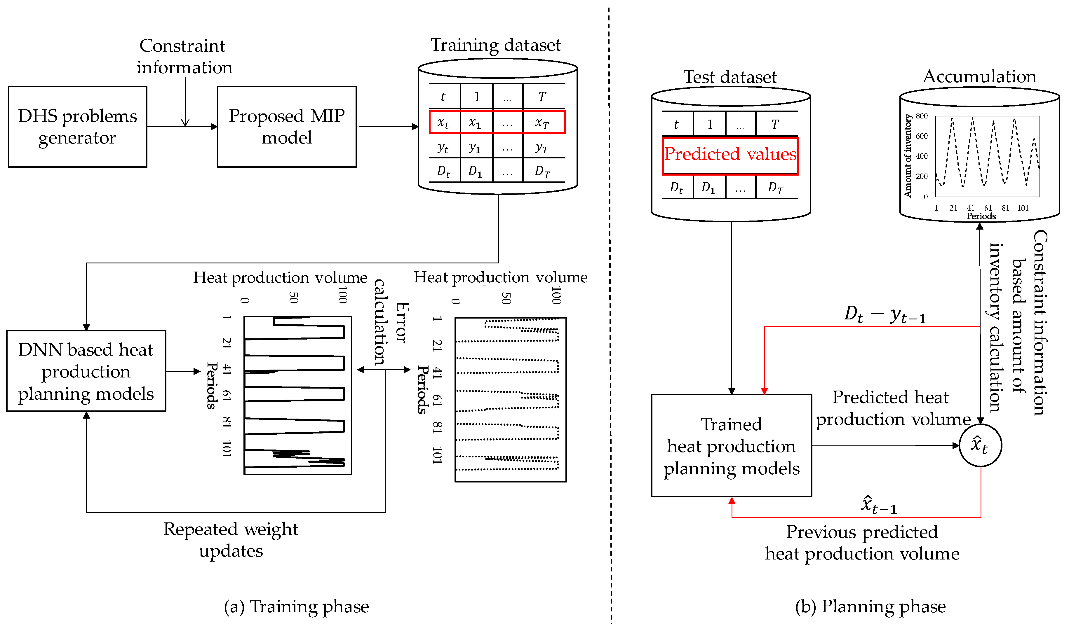
Figure 2 shows the details of the two-phase DNN framework with the training and planning phases. The first training phase consists of the DHS (district heating system) problem generator, the proposed MIP model, and the DNN planning model. In the beginning of the first training phase, the DHS problem generator produces a variety of heat production problems by changing the initial heat inventory $q_0$ and heat demands $D_t$ for the planning horizon. Then, the MIP model is executed to solve the problems generated by the DHS problem generator using commercial mathematical programming solvers. For the given input parameters including $q_0$, $D_t$ and other cost parameters, the MIP model yields solutions which will be used as a training dataset composing of inventory $q_t$, heat production $x_t$ and other production state variables $y_t$, $z_t$ and $w_t$. Then, the DNN planning model learns to minimize the differences between the optimal heat production volume $x_t$ and the predicted heat production volume ${\widehat{x}}_t$ by using the input variables including hourly demand $D_t$, hourly heat production cost, and previous heat production volume $x_{t-1}$. Since the predicted heat production schedule is near optimal solution from the MIP model, the DNN planning model trained by the schedule is expected to provide good solutions quickly in the test phase. After training, the algorithm keeps the best DNN parameter set for the training data.

In the second planning phase, the DNN planning model with the pre-trained parameter set is used to generate schedules for the cost and state parameters of the test data set. The trained DNN model predicts the heat production level at time t, ${\widehat{x}}_t$, using the previous heat production level $x_{t-1},$ and the previous status of accumulator, $D_t-y_{t-1}$. Note that the effective heat production estimation for the $t$-th period is directly related to its accuracy of the performances of the previous heat production estimation.

Note that the proposed solution mechanism does not include heat demand forecast algorithm in the framework and it is assumed that the heat demand forecasts for the planning periods will be given outside in the beginning of the planning process.

4.2. The Input and Output Features of DNN Model

A DNN model consists of input, hidden and output layers, where hidden layers may contain multiple layers interconnected.

Table 2. Inputs and output used for the proposed heat production planning model development.

Categories	Attributes	Descriptions	Number of Features
Inputs	1	${\widehat{q}}_{t-1}$, initial inventory at the beginning of time t	1
	2	${\widehat{x}}_{t-1}$, heat production at time t-1	1
	3	$D_t,\dots ,D_{t+23}$, heat demand forecasts for the next 24 h	24
	4	$V_t,\dots ,V_{t+23}$, hourly production costs for the next 24 h	24
Output	1	${\widehat{u}}_{k,t}$, target heat production level indicator at time t	K

shows the elements of the input and output values of the DNN model. The output layer has four features related to the production level variables ${\widehat{u}}_{k,t},mm,l$. The target of the DNN model is to predict heat production level at time t, while keeping the constraints (2) to (10) feasible and minimizing the proposed cost value by choosing an appropriate production level. The heat production level is assumed to be one of the values in the set {0, Cmin, (Cmin + Cmax)/2, Cmax}. If it is desirable to adjust the level of production, the number of features in the output layer needs to change accordingly. The DNN model can be thought as a classification model, which predicts the target state at time t with the information of the state variables at time t-1.

The input layer have 50 features including the initial inventory and heat production status at the beginning of time t, ($q_{t-1}$, ${\widehat{x}}_{t-1}$), future heat demand forecasts for the next 24 h, $D_t,D_{t+1},\dots ,D_{t+23}$ and future heat production costs $V_t,V_{t+1},\dots ,V_{t+23}$. The number of features in the input layer depends on the number of production levels and the reason why we include 24-h demand forecasts and production costs is that we are trying to minimize the total cost of operations during the planning horizon. To do this, we need to consider future demands and costs in advance. Since the goal of the planning process is to optimize hourly production schedule for the entire planning horizon, we give 24-h demand forecasts and costs to the DNN model. Therefore, DNN model is to predict the production level at time t when the inventory and production status at time t-1 and the 24-h demand forecasts and costs are given. By predicting heat production volume $x_t$ one by one recursively, we can generate a planning solution for the planning horizon more than 24 h. In the beginning of the process, the proposed solution framework predicts the target production volume $x_t$ at time t with 24-h cost and demand forecasts for the periods (t, t + 23). Once we predict the target heat production volume $x_t$ at time t, we can proceed to predict the heat production volume $x_{t+1}$ at the next time t+1 using the predicted heat production volume $x_t$ as input. In this recursive process, the predicted heat production volume $x_t$ in the output layer of DNN model is supplied to the input layer of DNN model when predicting heat production volume $x_{t+1}$ at time t + 1.

Since DNN model now has information about the previous production level and inventory remaining at the heat storage as well as the future demand and cost forecasts, it could properly choose the production level ${\widehat{u}}_{k,t}$ at time t. Once we have information about the production level, we could calculate the production related variables $y_t$, $z_t$, and $w_t$ by the following equations.

$${\widehat{x}}_t={\displaystyle \sum }_{k=1}^K{F}_k·{\widehat{u}}_{k,t}$$

(15)

$${\widehat{y}}_t=\{\begin{array}{cc}1& if{\widehat{x}}_t>0\\ 0& otherwise\end{array}$$

(16)

$${\widehat{z}}_t=\{\begin{array}{l}1,if{\widehat{y}}_t=1and{\widehat{y}}_{t-1}=0\hfill \\ 0,otherwise\hfill \end{array}$$

(17)

$${\widehat{w}}_t=\{\begin{array}{l}1,if{\widehat{y}}_t=0and{\widehat{y}}_{t-1}=1\hfill \\ 0,otherwise\hfill \end{array}$$

(18)

In addition, we can infer the remaining decision variables $q_t$, $r_t$, and $s_t$ as follows.

$${\widehat{q}}_t=\{\begin{array}{ll}A{C}_{max}\hfill & if{\widehat{q}}_{t-1}+D_t-{\widehat{x}}_t\ge A{C}_{max}\hfill \\ {\widehat{q}}_{t-1}+D_t-{\widehat{x}}_t\hfill & if{\widehat{q}}_{t-1}+D_t-{\widehat{x}}_t>A{C}_{min}and{\widehat{q}}_{t-1}+D_t-{\widehat{x}}_t<A{C}_{max}\hfill \\ A{C}_{min}\hfill & if{\widehat{q}}_{t-1}+D_t-{\widehat{x}}_t\le A{C}_{min}\hfill \end{array}$$

(19)

$${\widehat{r}}_t=\{\begin{array}{ll}{\widehat{q}}_{t-1}+D_t-{\widehat{x}}_t-A{C}_{max}\hfill & if{\widehat{q}}_{t-1}+D_t-{\widehat{x}}_t\ge A{C}_{max}\hfill \\ 0\hfill & if{\widehat{q}}_{t-1}+D_t-{\widehat{x}}_t<A{C}_{max}\hfill \end{array}$$

(20)

$${\widehat{s}}_t=\{\begin{array}{ll}A{C}_{min}-\left({\widehat{q}}_{t-1}+D_t-{\widehat{x}}_t\right)\hfill & if{\widehat{q}}_{t-1}+D_t-{\widehat{x}}_t\le A{C}_{min}\hfill \\ 0\hfill & if{\widehat{q}}_{t-1}+D_t-{\widehat{x}}_t>A{C}_{min}\hfill \end{array}$$

(21)

The DNN model is trained to predict heat production level $u_{k,t}$ at time t for the given parameters and the remaining decision variables $x_t$, $y_t$, $z_t$, $w_t$, $q_t$, $r_t$, and $s_t$ can be derived accordingly using the simple equations explained above. Therefore, we can predict production-related decisions for the entire planning horizon sequentially by predicting production level at each period and updating variables accordingly.

4.3. Structure of the Deep Neural Network for Planning

In this section, we outline the detailed structure of the DNN model as shown in Figure 3. The model consists of an input layer, five hidden layers, and an output layer, where nodes between adjacent layers are fully connected. Since the performances tend to vary according to the number of neurons and hidden layers, the number of layers and neurons in each layer are simultaneously determined by repeat trials [22]. In this study, by referring [19,23] we tested the DNN model training by varying the number of neurons and hidden layers to choose the best configuration. The number of layers were 4 to 7 in the references [19,23] and, in our setting, the proper number was set to five layers based on the preliminary experiments. The number of neurons in each layer is determined referring to the references [19,23] as well. If input data set changes, it is recommended to adjust the number of layers accordingly with initial experiments.

At first, each node in the input layer are corresponding to the input values related to attributes introduced in Section 4.2. For a node in the hidden layer, its input values which are calculated as the output values from its previous layer are used. A node in the output layer also utilizes the output values propagated from its previous layer as the input values and yields as the final estimation of the heat production. Here, we apply the rectified linear unit (ReLU) in the hidden and Softmax in the output layers. ReLU function was known to be effective in preventing gradient vanishing and radiant exploding problems in training process [24], and Softmax is widely used as classifier in classification problems [25,26,27].

The training process of the DNN model updates the weights of each hidden layer in the network gradually by minimizing the difference between the actual heat production level $u_{k,t}$ and the predicted heat production level ${\widehat{u}}_{k,t}$ The final output value is predicted by softmax function as presented in Equation (22), where $e^{{\widehat{u}}_{k,t}}$ is the estimation of heat production level obtained based on the highest probability value among the probability values of the actual heat productions $e^{u_{k,t}}$.

$$\mathsf{\sigma }\left({\widehat{u}}_{k,t}\right)=\frac{e^{{\widehat{u}}_{k,t}}}{{{\displaystyle \sum }}_{k=1}^K{e}^{u_{k,t}}}$$

(22)

To obtain the optimized weights in the hidden and output layers, the difference between the actual heat production level $u_{k,t}$ and the predicted heat production level ${\widehat{u}}_{k,t}$ is calculated by weighted categorical cross-entropy function. In addition, Adam optimizer manages how much the weights are updated based on the weighted categorical cross-entropy values for each training iteration. The back propagation approach is also adopted to optimize the weights for the proposed DNN model [2]. In this approach, the weighted categorical cross-entropy based difference value (loss function) is obtained by using Equation (23), where ${\tau }_k$ represents the weight value for the production level $u_{k,t}$.

$$Loss=-{\displaystyle \sum }_{k=1}^K{\tau }_k·(u_{k,t}·log{\widehat{u}}_{k,t})$$

(23)

In the planning phase, unlike the training phase, the trained DNN model uses the previous predicted heat production volume ${\widehat{x}}_t$ from its own self as the input value. When given value for each period, the predicted heat production volume ${\widehat{x}}_t$ is produced by computing the input values and the weights obtained in the training phase. The performances of the proposed heat production model are evaluated through the comprehensive experiment settings.

5. Computational Experiments

5.1. Data Set

To verify the efficiency and effectiveness of the proposed two-phase DNN model, it is applied to a regional office at KDHC (Korea District Heating Corporation, Gyeonggi-do, Korea), the largest district heating company in South Korea. KDHC is one of the companies owned by Korean government and provides district heating services to 17 demand regions with an installed capacity of 10,808 MW (9295.6 Gcal/h) in 2019, according to District Heating Business Handbook from Korea Energy Agency.

The data set used in the computational experiments in this section is derived from the one-year actual operational history of the selected demand region. In a typical regional office, a PLB (Peak Load Boiler) supplies heat to the corresponding demand area with a heat accumulator which balances the mismatch of supply and demand. Historical demand data for model building is sum of local heat demands including apartments and commercial buildings. Since the demand data is aggregated across demand region, specific demand characteristics are relaxed and the demand data is more tractable. We applied real cost parameters to the test scenarios while demands are generated from the real demand history by adding random noises to the real data. In the first training phase, the training data set has 1,440,000-h operational history and the validation data set has 360,000-h operational history data. In the second planning phase, the test data set has 12,000-h operational history. In the test run, we separate the 12,000-h data into 100 independent sets consisting of 120-h operations each. Figure 4 shows a sample operational history data given in the training phase. Each data set contains 120-h operations, which is five days per data set.

Table 3. Sample input and output values for the deep neural network (DNN) model.

Periods	Inputs				Output
	${\mathit{y}}_{\mathit{t}}$	${\mathit{d}}_{\mathit{t}}$	${\mathit{V}}_{\mathit{t}}$	${\widehat{\mathit{x}}}_{\mathit{t}\mathbf{-}\mathbf{1}}$	${\mathit{x}}_{\mathit{t}}$
1	470	68	60	0	77
2	405	63	60	${\widehat{x}}_1$	37
3	341	51	102	${\widehat{x}}_2$	43
4	312	41	102	${\widehat{x}}_3$	0
…	…	…	…	…	…
t	148	42	42	${\widehat{x}}_{t-1}$	40
…	…	…	…	…	…
120	730	0	0	${\widehat{x}}_{119}$	73

is a part of sample input and output values for the DNN model proposed. In each period (hour in this case), initial heat inventory status at the accumulator and heat demand will be used as input while heat production levels are used as target values for the DNN model. Note that the predicted heat production level ${\widehat{x}}_{t-1}$ is an output from the DNN model. Since the predicted heat production level is not supplied in the beginning of training and testing phases, the DNN model is applied to each period to forecast the production level, which will be supplied to the next-period DNN model as an input. This is somewhat similar to auto-regressive time-series forecast model. We tested the impact of the inclusion of the predicted heat production level in the input features in the computational experiments.

5.2. Experiment Settings

To test the effectiveness of the proposed model, we generated three model variants with different input attributes for the DNN model as defined in

Table 4. Attributes of DNN Model Variants.

Variant	Considered Attribute Types	Number of Input Features
DHP (DNN based heat production planning model)	1,3,4	49
DHPP (DNN based heat production model using predicted heat production)	1,2,3,4 (3: Predicted Heat Production)	50
DHPP2 (DHPP with on-off loss function weight differentiation)	1,2,3,4 (3: Predicted Heat Production)	50

. The first model DHP use pre-given input features excluding predicted heat production level. The second model DHPP includes the predicted heat production level in the input feature pools. The last model DHPP2 modifies ${\tau }_k$ in the loss function for the DNN model, where the parameters ${\tau }_k$ is set to 0.3 for the off state and 0.7/K for the remaining states (on states). In the DHP and DHPP model, the loss function parameters are set to the equal value regardless of the state. The reason of modifying the loss function parameters is to improve the on–off accuracy measure, which tests whether the given output from the DNN model classifies the on and off states appropriately. The main objective of the DNN model is to minimize the total cost and to classify the production level of each planning period. However, in the practice, it is equally import to estimate whether the production is on in any period. Due to demand uncertainties, it is inevitable to change production levels according to any demand changes but the on-and-off decision for each period is important to guide the overall planning process.

5.3. Experiment Results

As explained earlier, the DNN models has two modules including deep learning and mixed integer programming models. The deep learning part is tested in the Linux server using tensorflow 1.15 and python 3.8. The MIP models are optimized using xpress-mp solver in the OSX iMac Pro server with 128 GBytes memory and 18-core CPUs. The maximum runtime of the MIP model optimization is set to 300 s, which implies that the best feasible solution from the MIP solver might not be optimal in terms of the total cost measure. Therefore, the predicted solutions from the DNN model could be better than the solutions from the MIP model.

The DNN training and validation loss functions are shown in the Figure 5. Maximum number of the epochs is set to 100 and the loss functions show that the proposed DNN models are effectively trained. It is noted that the DNN models with heat production information in the input layer, DHPP and DHPP2, are more stable in terms of loss function compared to the model without heat production information in the input layer, DHP. Based on the learning curves, it seems that inclusion of heat production information in the input layer of the deep learning network is desirable to enhance stability of training process.

Table 5. Comparison of Cost and Accuracy Measures by Models.

Data Set	Total Cost				Level Accuracy			On–Off Accuracy
	MIP	DHP	DHPP	DHPP2	DHP	DHPP	DHPP2	DHP	DHPP	DHPP2
1	238,811	264,295	263,294	262,608	70.7%	75.5%	81.6%	87.0%	93.8%	94.5%
2	237,674	257,371	256,127	250,238	70.7%	73.4%	77.3%	87.0%	95.0%	96.2%
3	235,297	247,424	255,942	251,599	70.8%	74.4%	78.2%	87.5%	95.2%	97.3%
4	238,558	257,401	261,417	254,820	66.9%	72.7%	73.8%	85.2%	94.8%	95.6%
5	234,549	256,100	253,603	253,665	71.9%	77.8%	78.7%	86.6%	94.6%	92.6%
6	235,141	259,228	251,191	271,862	74.4%	76.4%	81.0%	89.9%	95.0%	94.9%
7	239,696	260,671	260,733	258,065	66.7%	73.3%	76.2%	84.9%	96.5%	95.1%
8	237,958	255,579	259,947	248,970	68.2%	72.6%	75.6%	87.2%	95.6%	96.4%
9	237,101	259,891	259,148	259,743	72.5%	77.2%	79.7%	85.1%	95.4%	95.4%
10	238,620	258,236	256,107	251,968	73.1%	78.8%	78.9%	82.8%	95.2%	95.9%
Average	237,341	257,620	257,751	256,354	70.6%	75.2%	78.1%	86.3%	95.1%	95.4%

summarized the performances of the given DNN models in terms of total cost, level accuracy and on–off binary accuracy measures. The total test instances are 100 cases of 120-h demand data. We grouped the test instances into a 10-data set and reported the average quality of the solutions for each data set in Table 5.

Table 5 shows that the total cost measures of three DNN models are slightly worse than those of the MIP models. Average total cost of DHPP2 is the best among the DNN models and is about 8% higher than that of the MIP model. In addition, DHPP2 shows better performances in terms of level and on-and-off accuracy measures. The production level accuracy of DHPP2 is 78.1% and the on–off state accuracy is 95.4%. These measures show that DHPP2 can effectively predict heat production level and production state for each planning period. Even though it takes time to train the DNN models, once we have the trained parameters, it only takes less than a second to predict production plans for the 120-h planning period using the DNN models proposed. As discussed, experimented in [1,6], the mixed integer programming model was effective to generate optimal solutions for the given scenarios but not able to find solutions quickly. As district heating systems have more constraints such as thermal storage storages, the problem becomes more complicated and it is necessary to relax hard constraints to find solutions efficiently [1]. However, the experiments in Table 5 show that the proposed solution framework would be effective even for long planning periods as well.

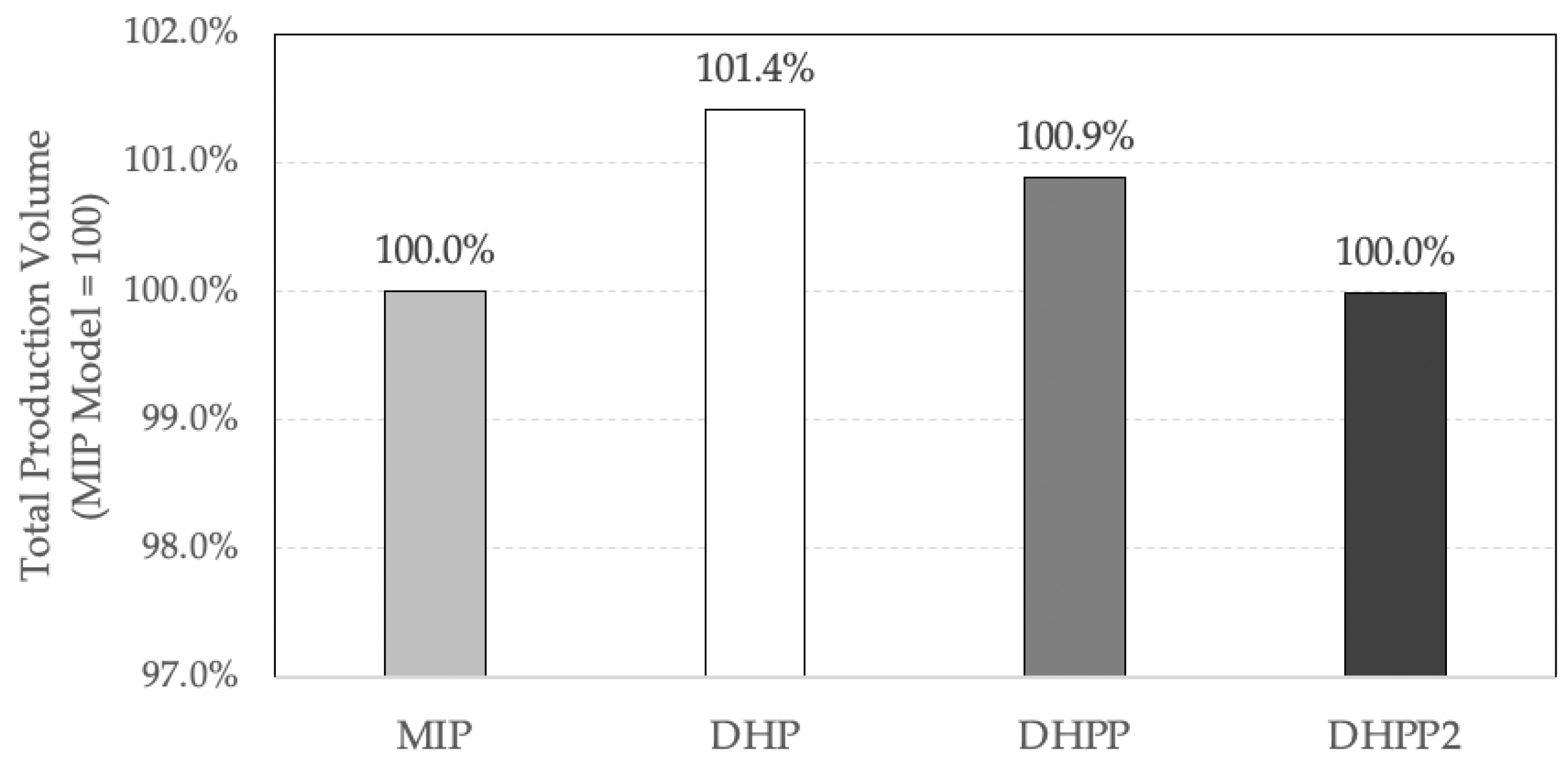
Figure 6 shows the comparison of the average production volume from each model. When the average production volume of the MIP model for the data is set to 100, DHP model generates solutions with slightly more heat production. The DHPP2 model is the closest to the MIP model.

6. Conclusions

In this study, we proposed deep learning based heat production planning models for a district heating system. Traditionally, optimization based heuristic algorithms were devised and applied to the heat production planning problem. Mixed integer programming models provided near optimal solutions, while it takes a while to generate solutions due to the characteristics of the underling solution mechanism. This inefficiency motivates development of efficient heuristic algorithms, but the solution qualities of these heuristics were insufficient in some problem settings. Therefore, we developed a two-phase solution mechanism, where deep learning algorithm is applied to learn optimal solutions from mixed integer programming models. By generating huge set of training instances using the optimization module, it was expected to train the deep learning module properly.

In the computation analysis, we tested the two-phase DNN model with test data instances collected from a district heating company in Korea. The test data set consists of 1,440,000-h operational history for training, 360,000-h operational data for validation and 12,000-h data for testing. To validate the effectiveness of the DNN model, we proposed three DNN model variants for the DNN model by varying input features and loss functions. The computation tests showed that the proposed DNN models were successful to generate fairly good solutions, which are comparable to the solutions from the MIP optimization model. The DNN model with predicted heat production level and on–off loss function modification (DHPP2) was shown to be better in terms of total cost and accuracy measures. In addition, the DNN models quickly predicted 120-h planning solutions in the second planning phase.

In real business practices, it is important to generate solutions quickly with less expensive way of computation. Even though the MIP model could generate near optimal solutions in the 300-min run time restriction, when a quick calculation is necessary, the proposed DNN models could be one of alternatives. If a district heating system contains multiple production sites across regions, it would be beneficial to implement the proposed DNN model since the proposed model could be deployed to cheaper computational environments. Moreover, data from the dispersed districting heating sites could be used to train the DNN model.

However, the solution quality from the DNN model strongly depends on the quality of the input operation patterns when training the DNN model in the first phase. If the DNN model is trained with poor quality of operation patterns, the algorithm cannot predict future operation patterns properly. Therefore, it is quite important to generate good operation patterns for the training purpose in the beginning of the process. If any key problem parameter changes, the proposed solution algorithm need to re-generate operation patterns for the changed problem parameters such as demand pattern changes, cost parameter changes or facility capacity changes. If parameter changes frequently occur, the first phase of generating operation patterns may be too time consuming since the algorithm adopted mixed integer programming model. To overcome this restriction, it might be better to replace the mixed integer programming model with heuristic solution algorithms. By combining computationally-light heuristic algorithm with deep learning model, it would shorten the learning and planning processes. The current solution framework considers a unit district heating system which consists of single production facility and demand node. To consider a network of multiple facilities and demand nodes, the proposed solution framework needs to be modified. In addition, to improve the prediction accuracy, any further study about problem specific input parameter is recommended. For example, if type of demand nodes and ambient temperature information is included in the input layer of the DNN model, it might be helpful to improve prediction process in the training process.

References

- Sameti, M.; Haghighat, F. Optimization approaches in district heating and cooling thermal network. Energy Build. 2017, 140, 121–130. [Google Scholar] [CrossRef]
- Vesterlund, M.; Toffolo, A.; Dahl, J. Optimization of multi-source complex district heating network, a case study. Energy 2017, 126, 53–63. [Google Scholar] [CrossRef]
- Protić, M.; Shamshirband, S.; Petković, D.; Abbasi, A.; Kiah, M.L.M.; Unar, J.A.; Raos, M. Forecasting of consumers heat load in district heating systems using the support vector machine with a discrete wavelet transform algorithm. Energy 2015, 87, 343–351. [Google Scholar] [CrossRef]
- Fang, T.; Lahdelma, R. Evaluation of a multiple linear regression model and SARIMA model in forecasting heat demand for district heating system. Appl. Energy 2016, 179, 544–552. [Google Scholar] [CrossRef]
- Bouktif, S.; Fiaz, A.; Ouni, A.; Serhani, M. Optimal deep learning LSTM model for electric load forecasting using feature selection and genetic algorithm: Comparison with machine learning approaches. Energies 2018, 11, 1636. [Google Scholar] [CrossRef]
- Lesko, M.; Bujalski, W.; Futyma, K. Operational optimization in district heating systems with the use of thermal energy storage. Energy 2018, 165, 902–915. [Google Scholar] [CrossRef]
- Wang, H.; Wang, H.; Haijian, Z.; Zhu, T. Optimization modeling for smart operation of multi-source district heating with distributed variable-speed pumps. Energy 2017, 138, 1247–1262. [Google Scholar] [CrossRef]
- Mertz, T.; Serra, S.; Henon, A.; Reneaume, J.M. A MINLP optimization of the configuration and the design of a district heating network: Academic study cases. Energy 2016, 117, 450–464. [Google Scholar] [CrossRef]
- Qin, C.; Yan, Q.; He, G. Integrated energy systems planning with electricity, heat and gas using particle swarm optimization. Energy 2019, 188, 116044. [Google Scholar] [CrossRef]
- Franco, A.; Versace, M. Multi-objective optimization for the maximization of the operating share of cogeneration system in District Heating Network. Energy Convers. Manag. 2017, 139, 33–44. [Google Scholar] [CrossRef]
- Dorotic, H.; Puksec, T.; Duic, N. Multi-objective optimization of district heating and cooling systems for a one-year time horizon. Energy 2019, 169, 319–328. [Google Scholar] [CrossRef]
- Weinand, J.M.; Kleinebrahm, M.; McKenna, R.; Mainzer, K.; Fichtner, W. Developing a combinatorial optimisation approach to design district heating networks based on deep geothermal energy. Appl. Energy 2019, 251, 113367. [Google Scholar] [CrossRef]
- Sameti, M.; Haghighat, F. Optimization of 4th generation distributed district heating system: Design and planning of combined heat and power. Renew. Energy 2019, 130, 371–387. [Google Scholar] [CrossRef]
- Talebi, B.; Haghighat, F.; Tuohy, P.; Mirzaei, P.A. Optimization of a hybrid community district heating system integrated with thermal energy storage system. J. Energy Storage 2019, 23, 128–137. [Google Scholar] [CrossRef]
- Rahman, A.; Smith, A.D. Predicting heating demand and sizing a stratified thermal storage tank using deep learning algorithms. Appl. Energy 2018, 228, 108–121. [Google Scholar] [CrossRef]
- Lu, K.; Meng, X.R.; Sun, W.X.; Zhang, R.G.; Han, Y.K.; Gao, S.; Su, D. GRU-based encoder-decoder for short-term CHP heat load forecast. IOP Conf. Ser. Mater. Sci. Eng. 2018, 392, 062173. [Google Scholar] [CrossRef]
- Kuan, L.; Zhenfu, B.; Xin, W.; Xiangrong, M.; Honghai, L.; Wenxue, S.; Zijian, Z.; Zhimin, L. Short-term CHP heat load forecast method based on concatenated LSTMs. In Proceedings of the 2017 Chinese Automation Congress (CAC), Jinan, China, 20–22 October 2017; pp. 99–103. [Google Scholar]
- Marino, D.L.; Amarasinghe, K.; Manic, M. Building energy load forecasting using deep neural networks. In Proceedings of the IECON 2016-42nd Annual Conference of the IEEE Industrial Electronics Society, Florence, Italy, 23–26 October 2016; pp. 7046–7051. [Google Scholar]
- Ryu, S.; Noh, J.; Kim, H. Deep neural network based demand side short term load forecasting. Energies 2017, 10, 3. [Google Scholar] [CrossRef]
- Sandberg, A.; Wallin, F.; Li, H.; Azaza, M. An analyze of long-term hourly district heat demand forecasting of a commercial building using neural networks. Energy Procedia 2017, 105, 3784–3790. [Google Scholar] [CrossRef]
- Shi, H.; Xu, M.; Li, R. Deep learning for household load forecasting—A novel pooling deep RNN. IEEE Trans. Smart Grid 2017, 9, 5271–5280. [Google Scholar] [CrossRef]
- Lee, D.; Kim, K. Recurrent neural network-based hourly prediction of photovoltaic power output using meteorological information. Energies 2019, 12, 215. [Google Scholar] [CrossRef]
- Alvarez, J.M.; Salzmann, M. Learning the number of neurons in deep networks. Adv. Neural Inf. Process. Syst. 2016, 29, 2270–2278. [Google Scholar]
- Krizhevsky, A.; Sutskever, I.; Hinton, G.E. Imagenet classification with deep convolutional neural networks. Commun. ACM 2017, 60, 84–90. [Google Scholar] [CrossRef]
- Pyakillya, B.; Kazachenko, N.; Mikhailovsky, N. Deep learning for ECG classification. J. Phys. Conf. Ser. 2017, 913, 012004. [Google Scholar] [CrossRef]
- Socher, R.; Huval, B.; Bath, B.; Manning, C.D.; Ng, A. Convolutional-recursive deep learning for 3d object classification. Adv. Neural Inf. Process. Syst. 2012, 25, 656–664. [Google Scholar]
- Chan, T.H.; Jia, K.; Gao, S.; Lu, J.; Zeng, Z.; Ma, Y. PCANet: A simple deep learning baseline for image classification? IEEE Trans. Image Process. 2015, 24, 5017–5032. [Google Scholar] [CrossRef]