Article

Thermodynamic Analysis of a High-Temperature Latent Heat Thermal Energy Storage System

Mechanical Engineering, The University of Alabama, Tuscaloosa, AL 35401, USA
*
Author to whom correspondence should be addressed.
Energies 2020, 13(24), 6634; https://doi.org/10.3390/en13246634
Submission received: 4 November 2020 / Revised: 11 December 2020 / Accepted: 14 December 2020 / Published: 16 December 2020
(This article belongs to the Special Issue The Concept of Entropy and Its Application in Thermal Engineering)

Abstract

:
Thermal energy storage (TES) technologies are becoming vitally important due to intermittency of renewable energy sources in solar applications. Since high energy density is an important parameter in TES systems, latent heat thermal energy storage (LHTES) system is a common way to store thermal energy. Though there are a great number of experimental studies in the field of LHTES systems, utilizing computational codes can yield relatively quick analyses with relatively small expense. In this study, a numerical investigation of a LHTES system has been studied using ANSYS FLUENT. Results are validated with experiments, using hydroquinone as a phase-change material (PCM), which is external to Therminol VP-1 as a heat transfer fluid (HTF) contained in pipes. Energy efficiency and entropy generation are investigated for different tube/pipe geometries with a constant PCM volume. HTF inlet temperature and flow rate impacts on the thermodynamic efficiencies are examined including viscous dissipation effects. Highest efficiency and lowest entropy generation cases exist when when flow rates are lowest due to low viscous heating effects. A positive relation is found between energy efficiency and volume ratio while it differs for entropy generation for higher and lower velocities. Both efficiency and entropy generation decreased with decreasing HTF inlet temperature. The novelty of this study is the analysis of the effect of volume ratio on system performance and PCM melting time which ultimately proved to be the most dominant factor among those considered herein. However, as PCM solidification and melting time is of primary importance to system designers, simply minimizing entropy generation by decreasing volume ratio in this case does not lead to a practically optimal system, merely to decrease heat transfer entropy generation. Therefore, caution should be taken when applying entropy analyses to any LHTES storage system as entropy minimization methods may not be appropriate for practicality purposes.

1. Introduction

Thermal energy storage (TES) is a popular tool to help match short and long-term energy demands. There are a variety of applications for TES, such as space heating and cooling and hot water storage [1]. The underlying premise behind TES is that thermal energy, or lack thereof, can be stored by heating or cooling a storage substance at high or low temperatures. This thermal store can be utilized at a later time for heating and cooling purposes [2]. There are a good number of advantages of TES systems: they can increase the efficiency and reliability of energy systems as well as reduce the investment cost and dependency of fossil fuels [2,3].
TES systems can be classified as sensible (STES), latent heat (LHTES), and thermochemical. In LHTES systems, the storage medium changes phase, and energy is released or absorbed during the phase change. The main parameters affecting LHTES performance are the specific heat, latent heat and fusion/boiling temperature of the storage material. LHTES systems have higher energy storage density compared to those of STES systems, and the operation temperature is relatively small as heat transfer usually takes place at a constant temperature. There are three important components in a LHTES system: the phase change material (PCM), heat transfer fluid (HTF), and PCM container. The PCM plays a crucial role, and desired characteristics include large heat of fusion, large specific heat, large thermal conductivity in both phases, large density, cost, and long-term chemical stability [1,4].
There have been a significant number of experimental studies analyzing LHTES systems. A high temperature pilot plant to test different TES systems has been built in the University of Lleida (Spain) that contains two storage tanks, based on a shell–and–tube heat exchanger design. Oro et al. [5] and Gil et al. [6] conducted experimental studies in this plant to test a TES system using two different PCMs, and it was found here that d-mannitol stored more energy than that of hydroquinone. The authors carried out two studies [7,8] to investigate the average effectiveness and effective thermal conductivity enhancement of TES systems using two different storage tanks with fins and without fins. Hydroquinone was found to be better for solar cooling applications because of its high enthalpy, suitable phase change temperature range and little subcooling [9]. Peiro et al. [10] performed an experimental study to examine the efficiency of heat exchangers of a LHTES systems in parallel and counter flow conditions comparing HTF inlet temperatures. Here, the authors found that counter flow with higher inlet temperature performs best.
Numerical analyses of LHTES systems have become a common tool to investigate heat transfer characteristics as of late. Sodhi et al. [11] performed a numerical investigation of the heat and mass transfer characteristics of a high temperature PCM using a multi tube heat exchanger system varying the tube size and number of tubes. The authors claimed that increasing the number of tubes from 13 to 25 reduced charging and discharging times by 20% and 48%, respectively. A novel heat transfer enhancement technique has been defined by Niyas and Muthukumar [12] to improve performance of encapsulated LTHES systems. The numerical model, developed in COMSOL [13], was used to show that fewer capsules can produce similar or higher energy storage with lower charging and discharging times. Meng et al. [14] carried out both experimental and numerical studies to examine the heat transfer characteristics of a tube-in-tank LHTES system. It was found here that heat transfer ratio increases with increasing the inlet velocity and the temperature variance between PCM and HTF. Niyas et al. [15] performed a numerical study to examine the storage characteristics of a LHTES system during charging and discharging periods changing the HTF inlet temperature, and flow rate. Here, the impact of HTF inlet temperature on melting and freezing time is greater than that of flow rate.
Energy and exergy analyses are often used to analyze TES systems from a thermodynamic standpoint. In order to undertake exergy analyses, entropy generation must be examined carefully to find locations of irreversibilities. Jegadheeswaran et al. [16] provided an intensive review on the exergy based evaluation of LHTES systems. The authors concluded that entropy generation is lower when the temperature difference between HTF inlet temperature and PCM temperature is lower for higher velocity cases. A numerical study by Elisa et al. [17] investigated design improvement of a shell-and-tube LHTES from an entropy generation standpoint, looking at finned and un-finned heat exchangers. The solidification time is reduced by 16% by improving the design of the fins, and it was concluded that entropy generation increases when the number of fins is increased. Riahi et al. [18] compared the exergy efficiencies of sensible and latent thermal energy storage systems, finding that PCM storage provides opportunities to minimize irreversibilities. An experimental study of a shell and helical heat exchanger has been performed by Rahimi et al. [19] to investigate the effect of helical diameter and temperature on the exergy efficiency of a LHTES system. The authors found that higher exergy efficiency (close to 95%) can be achieved when the helical diameter is lower. The authors also claimed a negative relation between PCM average temperature and entropy generation. MacPhee and Dincer [20,21,22] performed numerical studies to investigate thermodynamics efficiencies of encapsulated ice thermal energy storage system. Furthermore, the authors inspected the impact of viscous heating on the energy and exergy efficiencies as well as on entropy generation. The authors claimed that entropy generation decreases with decreasing flow rate and increasing the inlet temperature for charging process.
In this present work, a three-dimensional numerical LHTES model has been created to investigate the impacts of HTF inlet temperature, volumetric flow rate (VFR), and volume ratio (VR) of PCM to HTF domain on energy efficiency and entropy generation. ANSYS Fluent was used to simulate the cases, good agreement was found when comparing to a recent similar experimental study. Although other works exist that investigate the effect of temperature and flow rate on LHTES performance, geometry effects related to the performance varies for each study. The novelty behind this study is the focus on volume ratio, defined as the ratio of PCM to HTF volume, incorporating viscous dissipation losses, in energy efficiency and entropy generation along with the other two parameters. There are no known studies considering this volume ratio in this geometrical setting, and weighing losses comparing volume ratio to other factors such as HTF flow rate and temperature, on overall system performance in terms of energy efficiency and entropy generation.

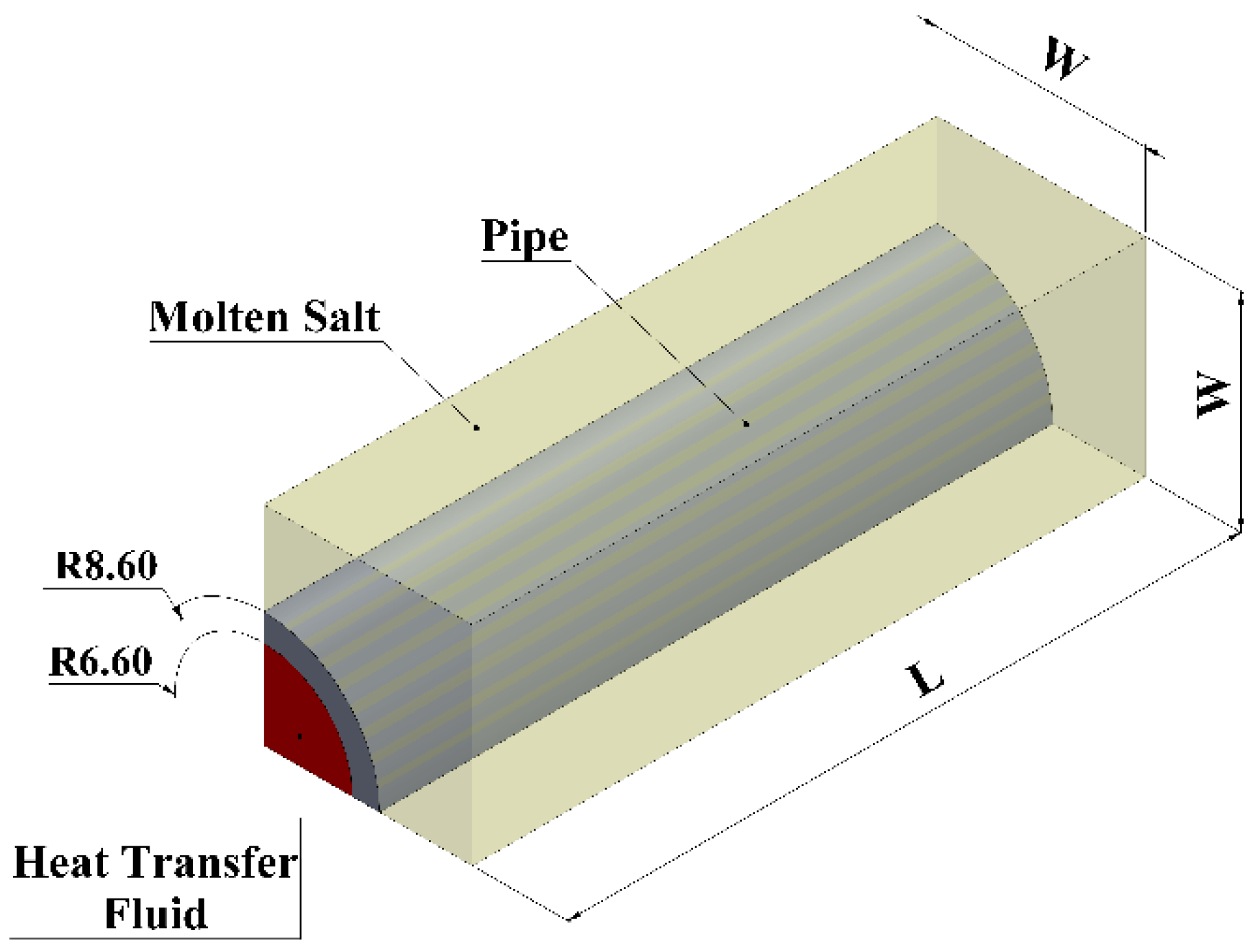
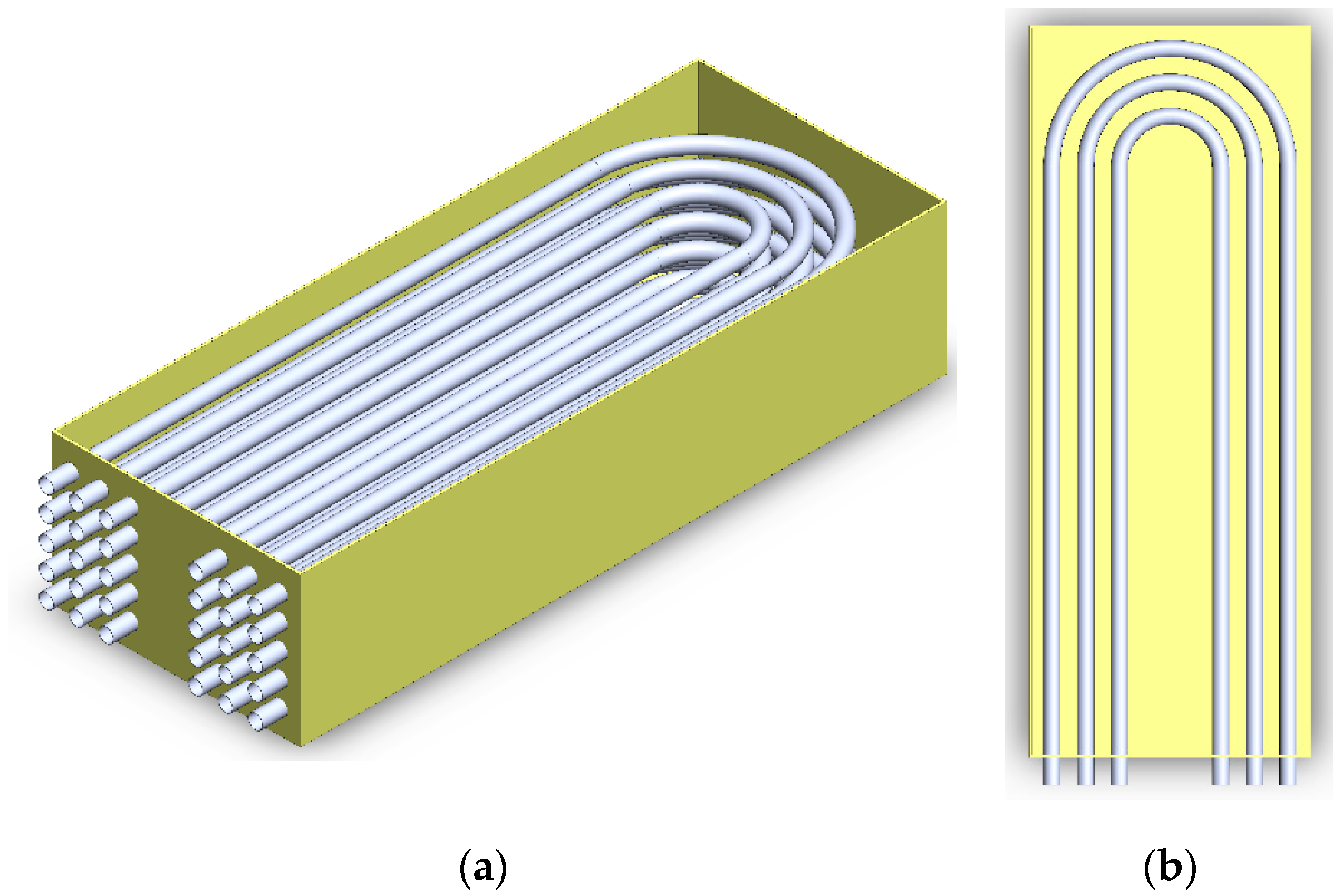
2. Mathematical Modeling

The numerical model created to store thermal energy in a molten salt using FLUENT is as shown in Figure 1. Although the geometry is essentially a shell-and-tube heat exchanger, only a quarter of a pipe is modeled to decrease computational cost. Here, hydroquinone is selected as a PCM due to its high enthalpy of fusion and melting temperature range. A synthetic thermal oil, Therminol VP1, is used as an HTF and stainless-steel piping separates the PCM and HTF. The property details of materials can be seen in Table 1. There are two processes considered in this study, charging and discharging. In the former, the HTF transfers thermal energy to the PCM and in the latter, the PCM releases thermal energy back to the HTF.
The impact of various input parameters on heat transfer and thermodynamic efficiency are explored by keeping the PCM volume constant at 236 mL (236,800 mm3) and the pipe inner and outer-radius constant at 6.6 mm and 8.6 mm, respectively. The PCM volume is constant in order to compare and validate result with a similar study [8], and the volume ratios of the PCM to HTF are varied from 1.5 to 30. More details about the volume ratio, length (L), and width (W) for all cases considered herein are shown in Table 2 and Figure 1.

2.1. Governing Equations

The continuity, momentum, and energy equations must be solved for the given transient model. This study assumes constant thermophysical properties, as seen in Table 1, as well as negligible radiation and gravitational effects. The energy equation for the HTF is as follows:
ρ H T F D h H T F D t = D p D t + k H T F 2 T + Φ
Here, Φ represents the viscous heating function, which results from shear stresses in the fluid:
Φ = μ [ 2 ( u x ) 2 + 2 ( v y ) 2 + 2 ( w z ) 2 + ( v x + u y ) 2 + ( w y + v z ) 2 + ( u z + w x ) 2 ]
Mass and momentum conservation for the HTF are given by Equations (3) and (4), respectively.
V = 0
ρ H T F D V t = p + μ 2 V
The energy equation for the PCM and pipe (containing the HTF) with the aforementioned assumptions are written as follows:
ρ p i p e D h p i p e D t = k p i p e 2 T
ρ p c m D H p c m D t = k p c m 2 T
In order to solve energy equations of the solidification and melting models, the enthalpy–porosity technique [23,24] is used, which evaluates enthalpy rather than temperature. Since there will be a phase change in the PCM, the enthalpy of the PCM, Hpcm, is the summation of the sensible enthalpy, h, and the latent heat enthalpy Hl.
H p c m = h + H l
Here, the sensible enthalpy, h, can written as:
h = h r e f + T r e f T C p d T
Here, href represents the reference enthalpy at the reference temperature, and the latent enthalpy term is evaluated using the liquid fraction:
H l = φ L
In the enthalpy–porosity method, the liquid fraction is determined for each iteration in all cells instead of tracking the solid/liquid interface explicitly. The range of liquid fraction changes from φ = 0 when T < Tsf to φ = 1 when T > Tsf.
φ = { 0   if   T < T s       C o m p l e t e y     S o l i d 1   if   T > T l       C o m p l e t e l y   L i q u i d ( T T s f ) / ( T l T s f )   if   T l > T > T s       S o l i d   a n d     L i q u i d }

2.2. Thermodynamic Analysis

In this study, energy and entropy analyses are undertaken to gain a better understanding of the location and severity of system losses. Only viscous dissipation losses are considered herein, though heat leakage can be a factor [25,26,27,28] but this becomes less pronounced as system size increases. Energy and entropy analyses are conducted in a similar format as in [21,29].

2.2.1. Energy Analysis

With the assumptions outlined earlier, the overall energy balance equation during charging or discharging processes are as follows:
Δ E s y s = E i n E o u t = U i n U o u t
At any time, the energy change in the system can be calculated by considering each material in the domain. Here, the HTF energy change incorporates the total mass existent at the initial state plus any mass flow that has entered during the simulation:
Δ E s y s = Δ E H T F + Δ E P i p e + Δ E P C M
Δ E H T F = m H T F C H T F ( T ¯ H T F T H T F , i n i )
Although it is possible to use Equation (13) to calculate energy changes in any domain, it is somewhate simpler and equivalent to use software capabilities to moinitor the heat transfer from fluid to the pipe as well as from pipe to the PCM.
Δ E P i p e = 0 t Q P i p e d t = i = 0 t Q P i p e , t
Δ E P C M = 0 t Q P C M d t = i = 0 t Q P C M , t
The energy efficiency of each process can then be calculated separately. Since the purpose of charging is to add thermal energy to the PCM domain, the charging energy efficiency is as follows:
η c h = E d e s E t o t a l = Δ E s y s H i n H o u t = Δ E s y s U i n U o u t + V ( P i n P o u t )
Here, U, H, V, and P are the internal energy, enthalpy, volume and pressure, respectively. In the discharging process, the desired energy represents the enthalpy change in the HTF, so the energy efficiency is written as follows:
η d i s = E d e s E t o t a l = H i n H o u t Δ E s y s = U i n U o u t + V ( P i n P o u t ) Δ E s y s
Since the majority of calculated efficiencies were well over 99% as a result of relatively low viscous dissipation, the efficiencies in this study were “contracted” or artificually decreased so as to look at the last percentile.
η c o n = η 0.99 0.0001

2.2.2. Entropy Analysis

In a similar way, the entropy balance equation can be written as follows:
Δ S s y s = S i n S o u t + S g e n , h e a t
Here, the change in entropy of the system can be calculated by summing the entropy change in each material:
Δ S s y s = Δ S H T F + Δ S P i p e + Δ S P C M
where,
Δ S P C M = Δ E p c m T ¯ b , p c m = i = 0 t Q p c m , t T ¯ b , p c m
Δ S H T F = m H T F C H T F l n ( T ¯ b , H T F T i n i )
Δ S P i p e = m P i p e C P i p e l n ( T ¯ b , P i p e T i n i )
T ¯ b represents the bulk temperature for each material. The flow entropy change is then:
S i n S o u t = i = 0 t m ˙ H T F C H T F l n ( T i n T ¯ o u t , t )
The total entropy generation can be calculated by summing the entropy generation due to heat transfer and viscous dissipation, Sgen,heat and Sgen,vd.
S g e n _ t o t a l = S g e n , h e a t + S g e n , v d
The entropy generation as a result of viscous dissipation can be calculated as follows:
S g e n , v d = V ( P i n P o u t ) T ¯ b , H T F
Here, T ¯ b , H T F is the fluid bulk temperature, which is easily monitred using Fluent software.

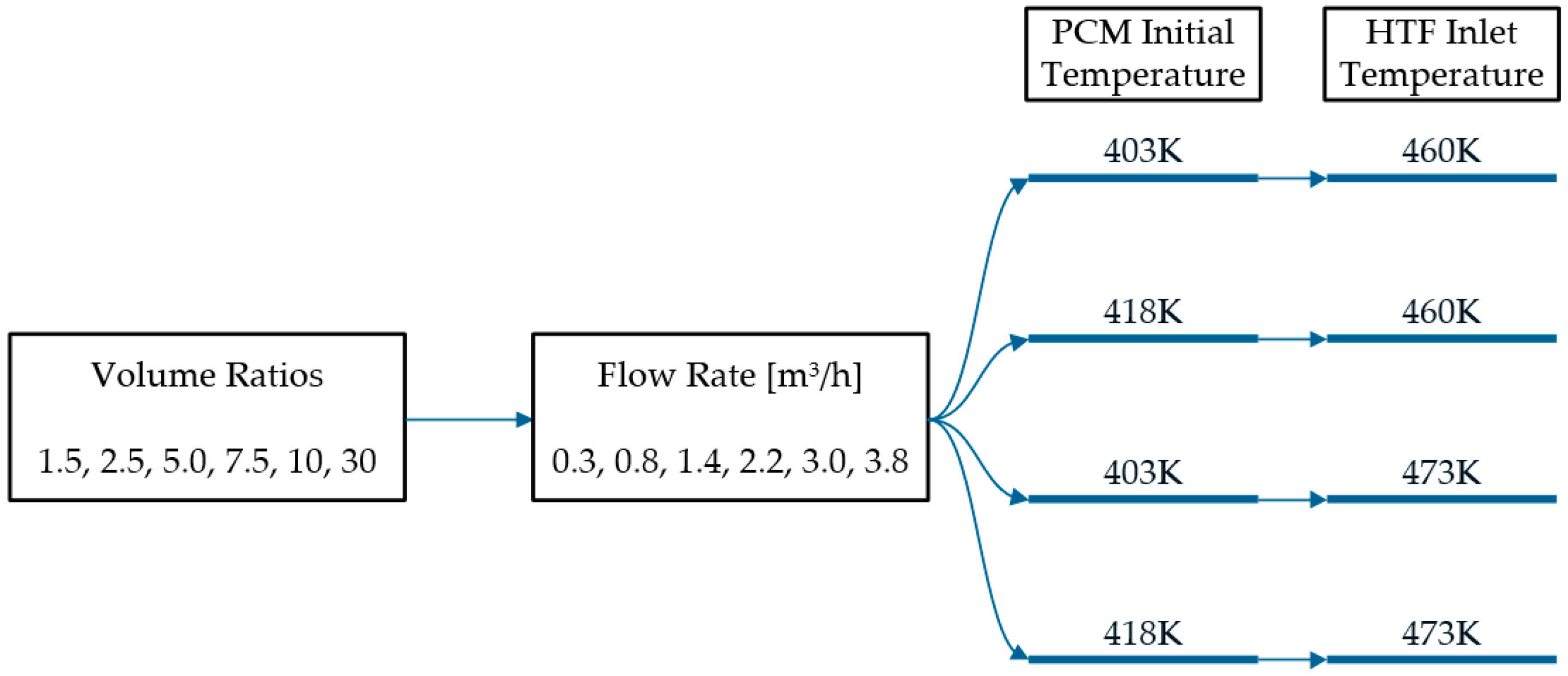
2.3. Boundary Conditions

Figure 2 shows the geometry and boundary conditions of the 3-D model. A fixed mass flow rate is applied to the inlet of the pipe. However, volumetric flow rate is used as a variable since mass flow rates vary with different inlet temperatures because of the density changes in the HTF. The volumetric flow rate is changed from 0.3 to 3.8 m3/h for the cases considered herein. The inlet temperatures of the HTF, Therminol VP1, are set to either 460 K or 473 K for the charging processes and 403 K or 418 K for the discharging process. A pressure—outlet boundary condition is used for the HTF outlet and coupled thermal boundary conditions were applied to the walls separating pipe and HTF/PDM. Due to symmetry, one quarter of the model is simulated. The initial temperatures of the HTF, pipe, and PCM domains are set to 403 K or 418 K for charging, and the final temperature after charging is used as the initial condition for the discharging case. A summary of all simulation variables is seen in Figure 3.

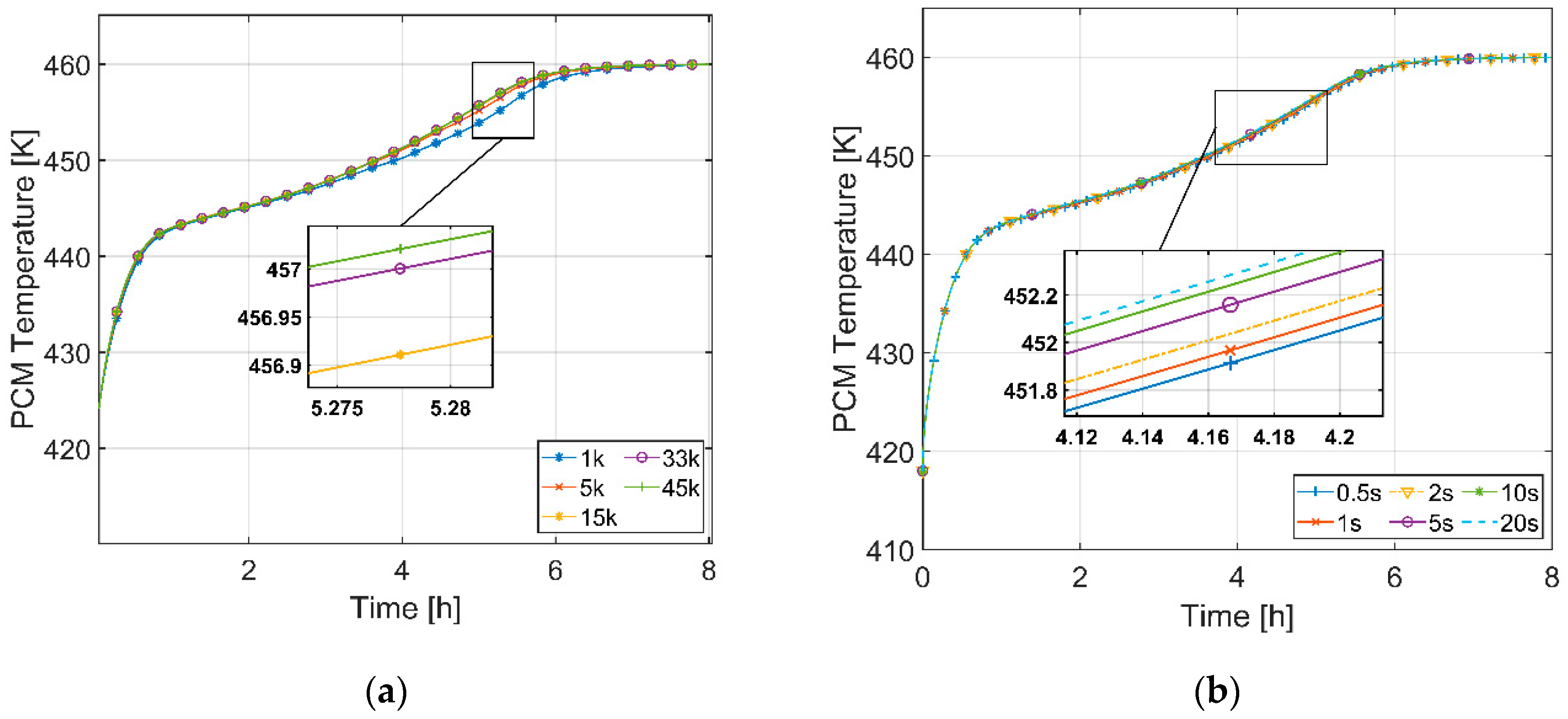
2.4. Mesh Generation, Independence Tests, and Solver Settings

Ansys Fluent is used to create the model and to generate the mesh. As shown in Figure 2, a structured mesh is used for all domains, with increased cell density near to fluid/solid interaces where high gradients are expected. Grid and time-step-size independence tests were performed to ensure the accuracy of the numerical model and volume-averaged PCM temperature was chosen to compare results. It was found here that 33,000 cells and a 5-s time-step-size were adequate for the given problem (see Figure 4). Here, both charging and discharging cases are performed for 8 h.
The SIMPLE (Semi-Implicit Method for Pressure Linked Equations) algorithm is used to solve the transient problem along with a second order upwind scheme for the discretization of pressure, momentum, and energy equations. In some cases, the HTF Reynolds number was in the turbulent regime, and a turbulence model was selected for these cases by simulating five commonly used models and choosing the PCM temperature results closest to experimental values as seen in [8] and explained in more detail in Section 3, see Figure 5b. Here, the k–w SST (shear stress transport) model is preferred and used whenever necessary to model turbulent flow for the remainder of the analysis. (see Figure 5b).
The authors also note that several simulations were also conducted to ascertain the effects of buoyancy (that is, natural convection) on simulated parameters. In all cases investigated herein, natural convection effects do not alter PCM temperatures by more than 2–3 K or charging/discharging times by more than 2–3%, validating the assumption of negligible gravitational effects in solver settings.

3. Results and Discussion
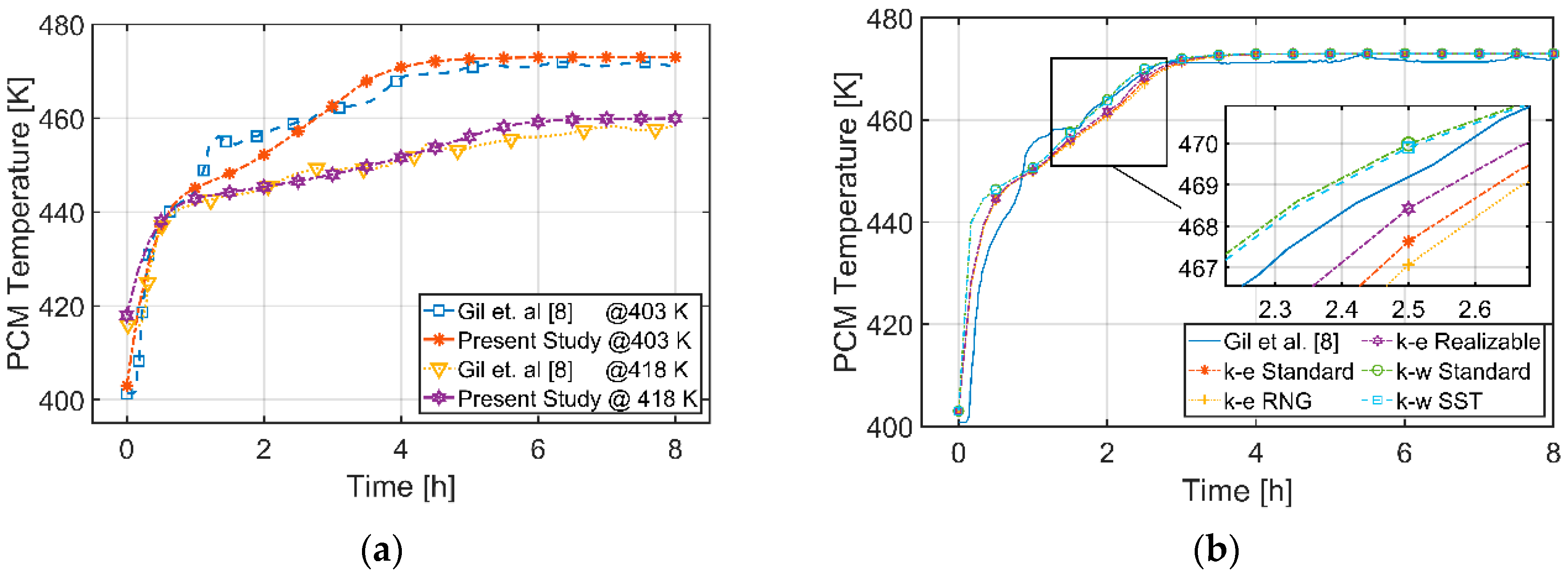
3.1. Validation

As mentioned previously, simulations are compared and validated with experimental findings from [8], and the experimental setup is reproduced graphically in Figure 6. In this study, a significant number of tests were performed using shell-and-tube heat exchangers, with and one without fins. This study compares the fin-less heat exchanger for validation purposes, using 2 of the 15 temperature sensors farthest from outer walls in Figure 6, and comparing to simulated PCM temperatures recorded in the appropriate cells of the computational domain. Since the experimental study [8] has been performed for both laminar and turbulent flow regimes, two volumetric flow rate cases were simulated. For laminar flow, a 1.4 m3/h volumetric flow, corresponding to a Reynolds number of 1633, was simulated to match experimental tests, and no turbulence modeling is utilized. Figure 5a shows the simulated temperatures compared to experimental values for the charging process in this case, for two initial PCM temperatures and HTF inlet temperatures. As seen in Figure 5a, PCM temperatures are found to be quite similar to experimental results.
For the turbulent flow regime, a flow rate of 3.0 m3/h is selected, corresponding to a Reynolds number of 3785. The aforementioned k–w SST model provides good agreement for all charging cases, though only one such case is shown in Figure 5b, along with other turbulence models investigated. The highest temperature deviation from experiments throughout charging was found to be 9 K.

3.2. Thermodynamic Efficiencies

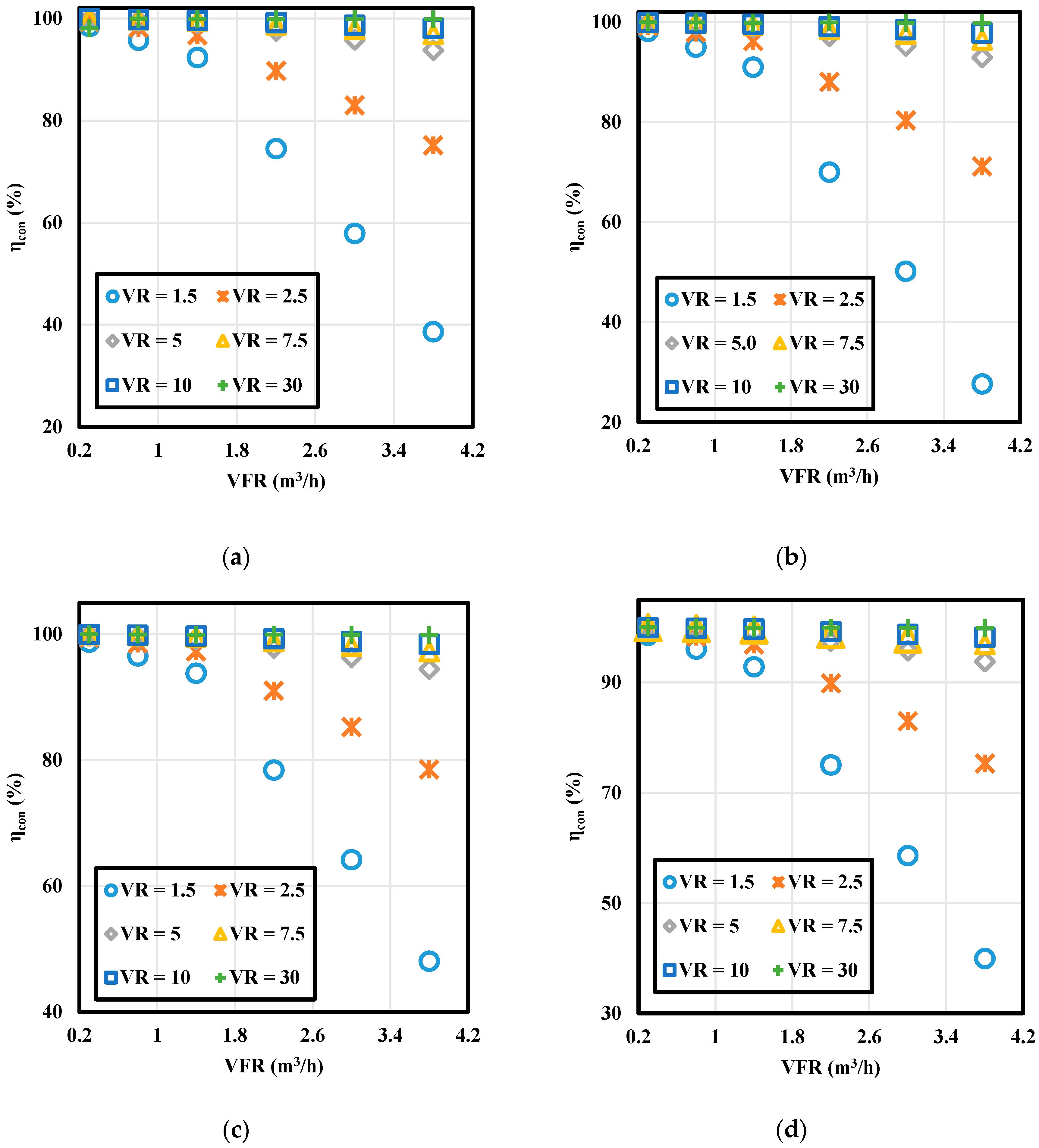
3.2.1. First Law Efficiency

To calculate energy efficiencies, Equations (11)–(18) are used; however, all energy efficiencies are obtained to be over 99% since each system is considered to be adiabatic; hence, only losses are resulted in by viscous heating which are significantly lower than stored energy content. Although energy efficiencies are over 99% in all cases, the viscous heating impact is discussed here using contracted energy efficiency (Equation (18)), which serve to “zoom in” on the last percentile of energy efficiency; the casual reader may conclude that system losses as described here are not substantial. This is one of the shortcomings of energy analyses for LHTES storage systems, as they do not account for irreversibility present in the system (which are more pronounced if lower “quality” thermal energy is stored). Regardless, the below discussion highlights some trends that aid in entropy analysis results of Section 3.2.2.
As can be seen from Figure 7, contracted energy efficiencies decrease with increasing volumetric flow rate due to the fact that higher flow rates cause higher bulk fluid velocity, hence more viscous dissipation in flow. The HTF inlet temperature impact on the contracted energy efficiency is also seen in Figure 7. Two different inlet temperatures and two different initial PCM temperatures are investigated here for different volume ratios and volumetric flow rates. It is not surprising that energy efficiencies are higher when the HTF inlet temperature is higher, since larger temperature differences between HTF and PCM results in higher heat transfer as expected (see: Newton’s Law of cooling).
As can be seen from Figure 8, the effect of volume ratio on the contracted energy efficiency is slightly more pronounced than that of HTF inlet temperatures. It should be pointed out that the lengths of both pipe and tank are equal; hence, the total HTF volume is lower when the volume ratio is higher. It is clear from Figure 8 that energy efficiencies increase with increasing volume ratio. The main reason for this phenomena is the low viscous heating effect on the higher volume ratio since the drop in the total pressure is quite low when the pipe (flow) length is small. However, there is an important point here; that the volume ratio effect on the energy efficiency mostly depends on the flow rate. For instance, when the volumetric flow rate is changed from 1.5 to 30, while the contracted energy efficiency increases from 98.00% to 99.99% for the case when the volumetric flow rate is 0.3 m3/h, it increases from 26% to 99% when the flow rate is 3.8 m3/h. Lastly, the contracted energy efficiencies are always higher during charging than for discharging since the viscous dissipation effect is higher during the discharging period.

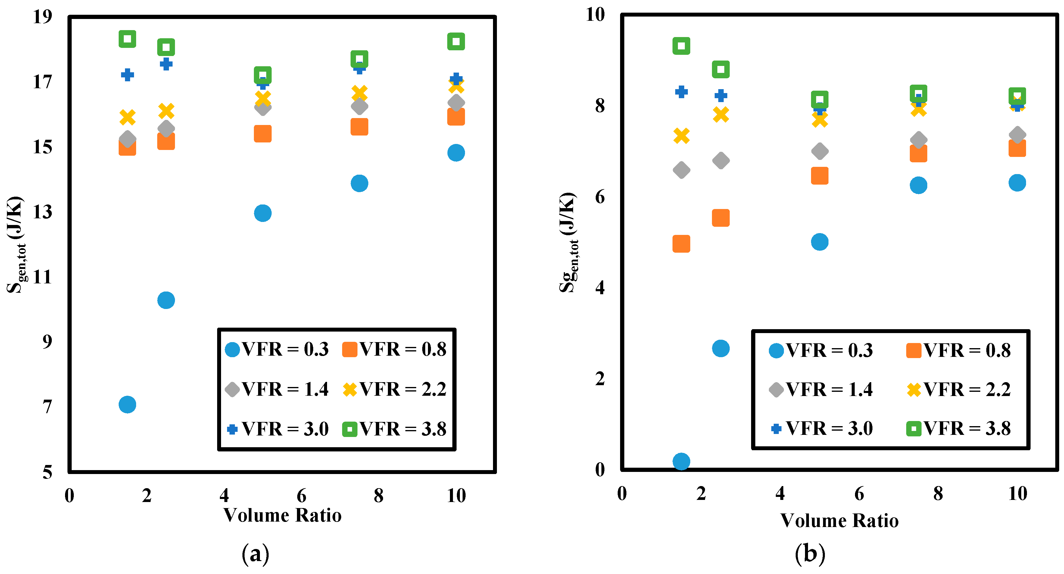
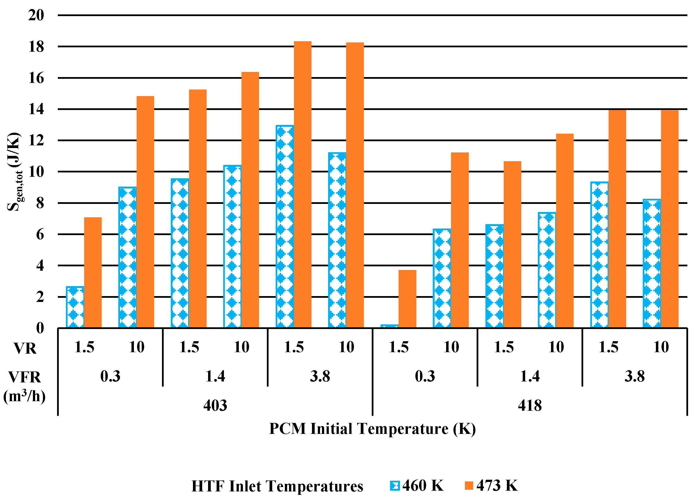
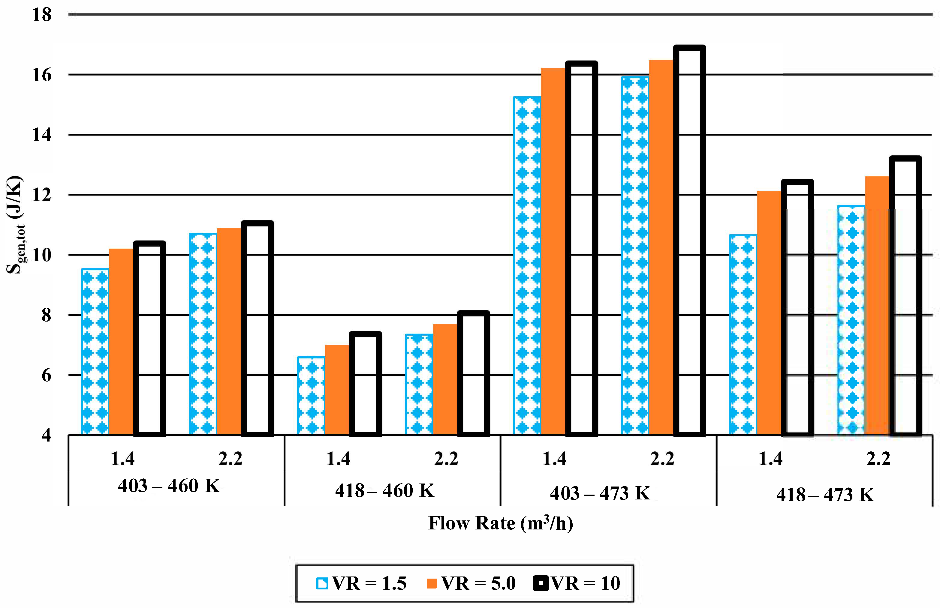
3.2.2. Entropy Generation

Although energy analyses are common, exergy and entropy analyses analyses may give more insight into system losses, since they may allow for better identification of location and severities of irreversibilities. In this case, entropy generation results from two irreversibilities: viscous dissipation and heat transfer. In this section, entropy generation resulting from of these two phonemena are discussed varying the parameters as defined in Figure 3. Equations (19)–(26) are used to calculate entropy generation as introduced by [21,29].
Figure 9 shows the total entropy generation due to heat transfer and viscous dissipation for varying volume ratio, flow rate, and temperature. Here, there is an increasing trend in the entropy generation with increasing volume ratio for lower flow rates. The reason for this phenomena is since higher volume ratios result in lower entropy change in the flow. As mentioned earlier, the total HTF volume is lower when the volume ratio is higher, and this causes lower entropy change in the flow. In other words, entropy change in the flow mainly depends on the outlet and inlet temperature of the fluid. When the volume ratio is higher, the length of the pipe will be lower, and the heat transfer from fluid to PCM will be lower. Since outlet temperature of the fluid is not as high as lower volume ratio cases, the flow entropy change decreases significantly. Moreover, since the HTF volume is not as high as lower volume ratio cases, the PCM melting time increases significantly for higher volume ratios (see Figure 12). Due to the fact that each system was charged for 8 h, none of the cases with volume ratios of 30 experienced full melting in 8 h. Therefore, these cases are not shown in entropy generation figures. Conversely, when the flow rate is higher, and experiences more viscous dissipation, total entropy generations decrease with increasing volume ratio. This is not surprising because entropy generation due to viscous dissipation increases with decreased volume ratio, as it is manifested in the pressure drop across the domain. One can notice that there is an increment in the entropy generation followed by a decrement for the case of 3.8 m3/h volumetric flow rate with increasing volume ratio. In this case, entropy change in the PCM is higher although entropy generation due to viscous heating is relatively low.
Another important consideration here is the HTF inlet temperature impact on the entropy generation as demonstrated in Figure 10. As mentioned before, four different cases performed here; while the initial temperature of the PCM is selected to be 403 K and 418 K, the HTF inlet temperature is 460 K and 473 K. It is clear from Figure 10 that, when larger temperature differences exist between the HTF inlet temperature and PCM temperature, total entropy generation is always greater since heat transfer from HTF to PCM is greater for larger temperature differences. It is more obvious in Figure 10 that while entropy generation increased with increasing volume ratio for lower flow rates, it decreases when the flow rate was 3.8 m3/h. It is important to note that entropy generation decreases when the volume ratio is increased since there will be lower entropy change in the PCM.
As stated previously, one of the main purposes of this study is to investigate the effect of viscous dissipation on the total entropy generation. Although viscous dissipation is neglected for lower flow rates in many studies, it could be very crucial as can be seen from Table 3. While the entropy generation due to heat transfer increased when the volume ratio is increased, entropy generation due to viscous dissipation decreased since the total HTF volume will be higher for lower volume ratios. It is not surprising that entropy generation attributed to viscous heating increases with increasing flow rate as a consequence of higher shearing in the fluid. Lastly, viscous dissipation effect on the total entropy generation is found to be more than 26% when the temperature difference between HTF and PCM is the lowest, and the volumetric flow rate and volume ratios are 0.3 m3/h and 1.5, respectively. Viscous dissipation effect in this case is very high, but the entropy generation due to heat transfer is very low due to lower heat transfer from the HTF to the PCM.

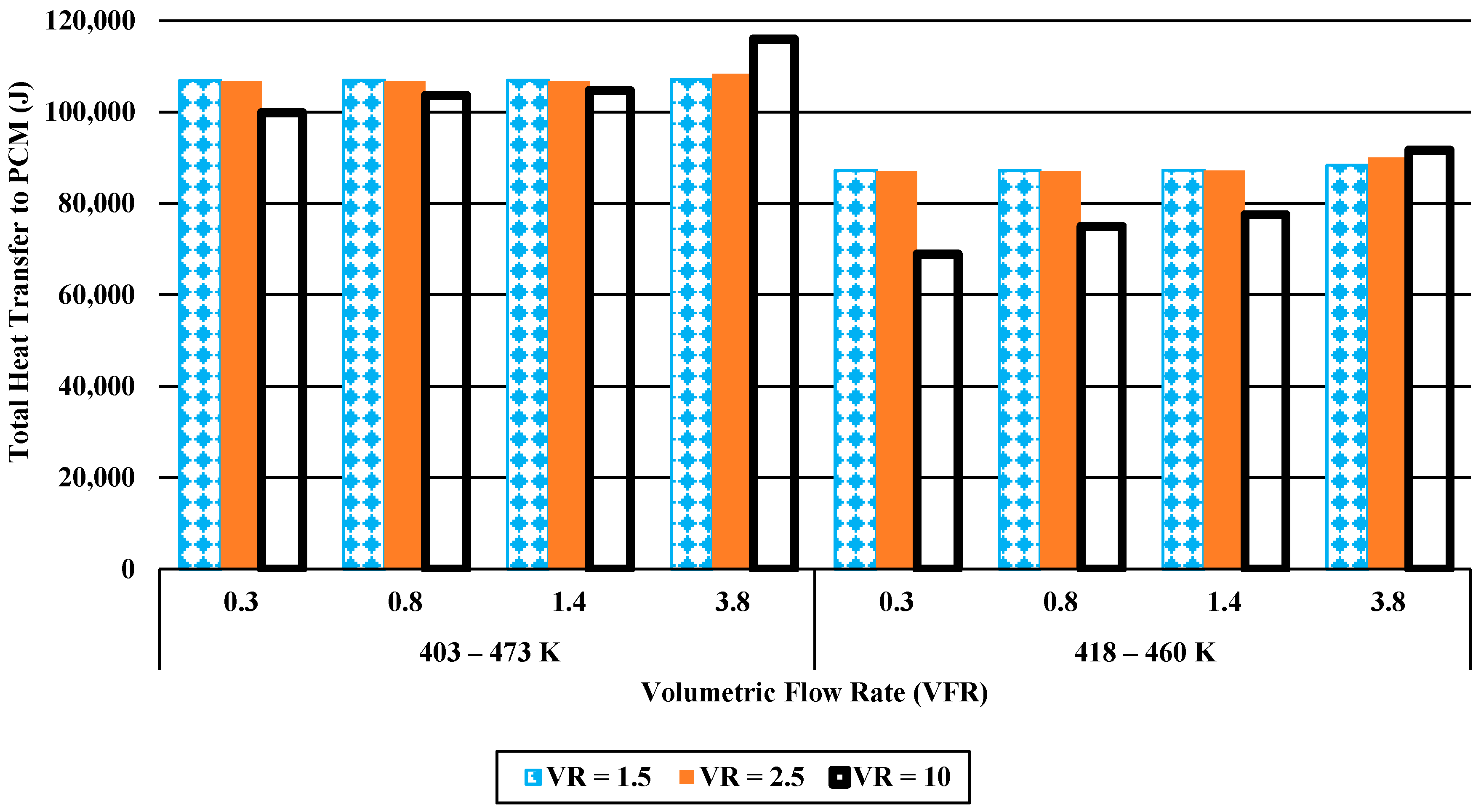
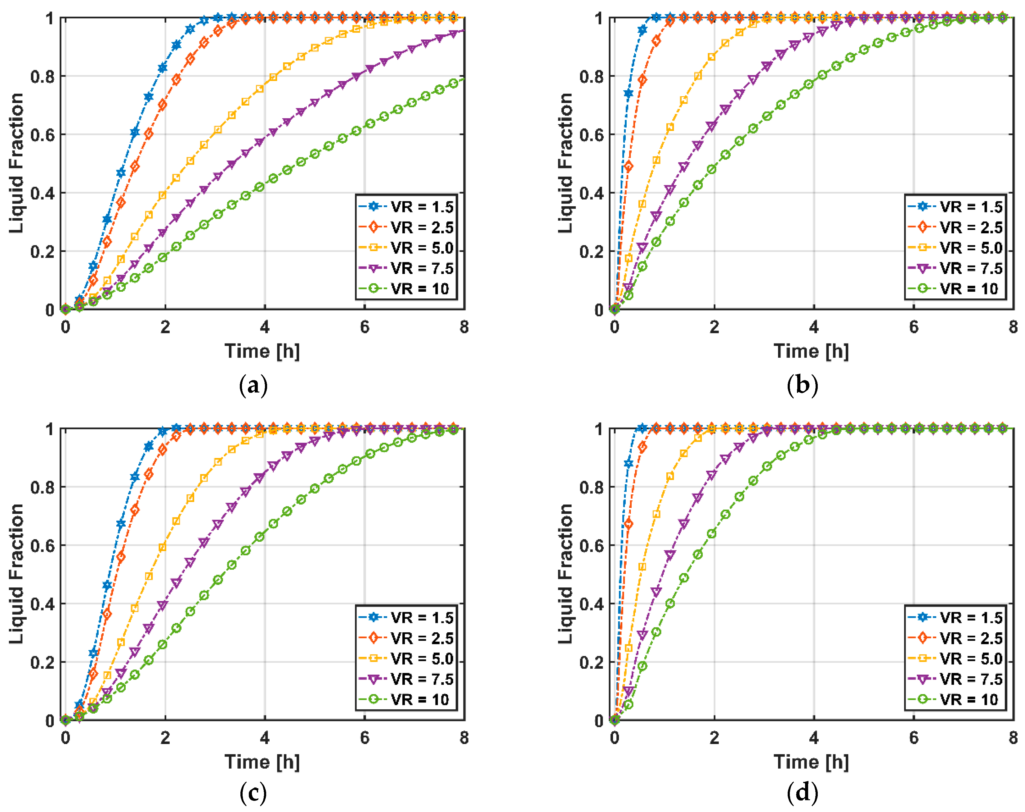
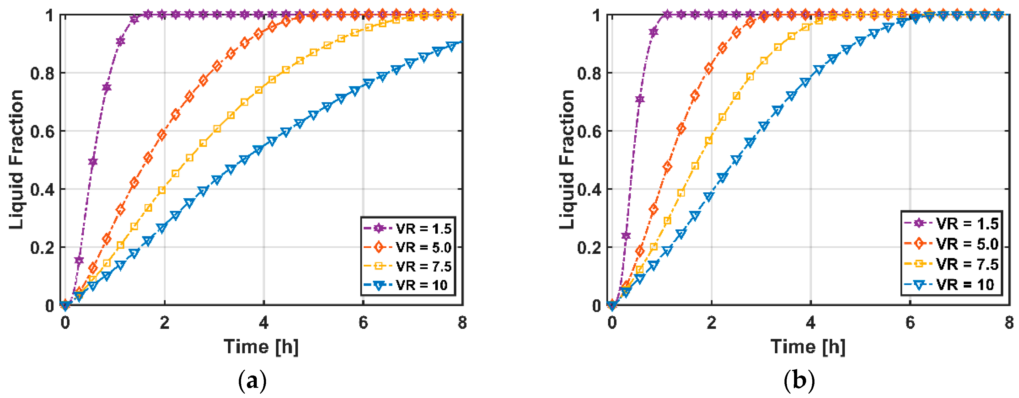
3.2.3. Total Heat Transfer and Melting Time

It is also important to discuss PCM melting times and stored energy, as they play a crucial role in system performance. As can be seen in Figure 11, total heat transfer (equivalently, stored energy) are always higher when the temperature differences are higher between the PCM and the HTF. Unsurprisingly, the same trend is also obvious for the volumetric flow rates. When the volumetric flow rate increases, more thermal energy can be transferred from HTF to PCM. However, there is an important point here when the volume ratio is inspected. While heat transfer amount increases with increasing volume ratio when the flow rate is higher (turbulent flow), it decreases with increasing volume ratio when the flow rate is lower (laminar flow). This is likely because when the volume ratio is lower the length of the pipe will be higher that results in higher HTF volume and higher heat transfer surface area. Since the HTF volume is higher, there will be more heat transfer from HTF to the PCM. When the volumetric flow rate is lower, there will not be enough time to melt the PCM for higher volume ratio cases; that will cause lower heat transfer rates.
Volume averaged liquid fraction is recorded for all simulations in the PCM, and is most affected by volume ratio, unsurprisingly. In Figure 12, two different temperature ranges and two different volumetric flow rates are used to compare PCM melting time while varying the volume ratios. The lowest volume ratios, which ultimately result in higher aspect ratios of the PCM storage system, do charge fastest, as do the simulations with higher flow rates and larger temperature differences. These findings suggest that, generally, when designing a PCM storage system for high temperature solar thermal storage, a lower volume ratio is desired for highest chance of fully charging the system.

3.2.4. Case Study

Although energy efficiency and entropy generation of parametric studies have been illustrated in the two previous sub-sections, the most efficient geometric model should be compared with the existing model in terms of entropy generation, especially since energy efficiencies of all cases have been found to be well over 99%. It should be noted that neither entropy generation nor energy efficiency of the reference study have been investigated. Hence, entropy generations were calculated using Equations (19)–(26) based on the PCM and HTF temperatures since the validation of the model is assumed to be reasonable as shown in Figure 5 and explained in Section 3.1. Besides entropy generation comparisons, liquefaction time will also be compared to examine melting times.
Figure 13 indicates the liquid fractions for two different PCM and HTF inlet temperature cases varying the volume ratio when the volumetric flow rate is 1.4 m3/h. It should be noted that the required time to melt the PCM decreases with decreasing volume ratio since the total HTF volume and heat transfer surface area are higher in that case. It should also be noted that the amount of energy that can be stored in the PCM will be different for different volume ratios as it was discussed in detail in Section 3.2.3. Furthermore, it is surprising that PCM melts faster when the HTF inlet temperature is 473 K even though the PCM initial temperature is lower in that case.
It is obvious from Figure 14 that the entropy generation of the reference model could be decreased by decreasing the space between the HTF tubes. To recall the definition of volume ratio, it represents the ratio of the PCM volume to the HTF volume that flows inside of the tubes. While the volume ratio of the reference model is 5.3, it has been varied from 1.5 to 30 in this work. One might think that decreasing the space between the tubes will results in lower energy storage in the molten salt, however, it will not be affected since the volume of the molten salt is kept constant in the proposed design by extending the lengths of the tube and PCM bath. Though not explicitly calculated here, the exergy efficiencies of the reference study are higher than 88% for all cases, which are quite high for LHTES applications. Nevertheless, the exergy efficiency still can be improved with lower entropy generation, in changing the design of the tubes. For example, entropy generation in the reference study can be decreased by 12% for a case that has a volumetric flow rate of 1.4 m3/h, and temperatures of PCM and HTF inlet of 418 and 473 K, respectively. Although 12% entropy generation decrement seems low, it will have a considerable effect on the potential energy when the system is applied/extended to a large scale. As can be seen from Figure 14, entropy generation is higher when the flow rate is higher due to viscous heating. Therefore, entropy generation can be decreased by decreasing the volume ratio and volumetric flow rate.

4. Conclusions

In this study, a numerical model has been created to store thermal energy in a shell and tube heat exchanger using the LHTES method. 288 simulations have been performed via ANSYS FLUENT varying the volume ratio of the PCM to HTF from 1.5 to 30, volumetric flow rate from 0.3 m3/h to 3.8 m3/h, and the PCM and HTF inlet temperatures from 403 K to 418 K, and 460 K to 473 K, respectively. Hydroquinone is selected as a PCM, and Therminol VP-1 is used as the HTF. The cases were simulated for 8 h charging and 8 h discharging. Energy efficiency, entropy generation, heat energy stored and PCM melting time analyses have been performed to find optimal designs. The important findings of this study have been listed as follows:
  • Due to the minor effect of viscous dissipation, energy efficiencies are over 99% in all cases.
  • While energy efficiencies decrease with increasing volumetric flow rate, entropy generations increase due to higher viscous heating with velocity. Volumetric flow rate shows a positive and negative relationship between heat transfer ratio and PCM melting time, respectively.
  • Whereas there is an increasing trend in the energy efficiencies with increasing volume ratio, the trend differs for lower and higher velocities for entropy generation.
  • While entropy generation increases with increasing volume ratio for lower flow rates, it decreases with higher flow rate.
  • Both energy efficiency and entropy generation increase with increasing HTF inlet temperature.
  • The effect of volume ratio on the energy efficiency is higher than that of HTF inlet temperatures.
  • PCM melting time decreases with decreasing volume ratio due to higher heat transfer surfaces.
  • Entropy generation is lowered with reduced volume ratio and decreased heat transfer rate. Since the purpose of the LHTES system is to store heat energy, entropy generation may then not be the most appropriate design tool as system costs for lower volume ratios will become prohibitive.

Author Contributions

The First Author (M.E.) designed the computational model, performed the simulations, validated, and analyzed the results as well as wrote and edited the article. The second author (D.W.M.) was M.E.’s research supervisor and facilitated each of these contributions. All authors have read and agreed to the published version of the manuscript.

Funding

This research received no external funding.

Conflicts of Interest

The authors declare no conflict of interest.

Abbreviations

Nomenclature
Cspecific heat (J/kg K)
Dpipe diameter (m)
Eenergy (J)
henthalpy (J/kg)
Htotal specific enthalpy (J)
kthermal conductivity (W/m K)
Llatent heat (J/kg)
mmass (kg)
Pstatic pressure (Pa)
Sentropy (J/K)
Qtotal heat transfer rate (W)
Ttemperature (K)
ttime (s)
tototal
Uinternal energy (J)
Vvolume (m3)
Greek Letters and Special Symbols
Δ“change in”
dead state
ηenergy efficiency
mass flow rate (kg/s)
ρdensity (kg/m3)
φliquid fraction
Subscript
concontracted
bbulk
chcharging
ddestroyed
desdesired
disdischarging
gengenerated
ininlet
iniinitial
lliquid
outoutlet
oreference
syssystem
vdviscous dissipation
HTFheat transfer fluid
VRvolume ratio
VFRvolumetric flow rate (m3/h)
LHTESlatent heat thermal energy storage
TESthermal energy storage
PCMphase change material

References

  1. Dincer, I.; Ezan, M.A. Heat Storage: A Unique Solution For Energy Systems; Green Energy and Technology; Springer International Publishing: Cham, Switzerland, 2018; ISBN 978-3-319-91892-1. [Google Scholar]
  2. Sarbu, I.; Sebarchievici, C. A comprehensive review of thermal energy storage. Sustainability 2018, 10, 191. [Google Scholar] [CrossRef] [Green Version]
  3. Mahmud, R.; Erguvan, M.; MacPhee, D.W. Underground CSP Thermal Energy Storage. In Proceedings of the ASME 2019 Power Conference, Salt Lake City, UT, USA, 15–18 July 2019; American Society of Mechanical Engineers: New York, NY, USA, 2019. [Google Scholar]
  4. Nomura, T.; Okinaka, N.; Akiyama, T. Technology of latent heat storage for high temperature application: A review. ISIJ Int. 2010, 50, 1229–1239. [Google Scholar] [CrossRef] [Green Version]
  5. Oró, E.; Gil, A.; Miró, L.; Peiró, G.; Álvarez, S.; Cabeza, L.F. Thermal Energy Storage Implementation Using Phase Change Materials for Solar Cooling and Refrigeration Applications. Energy Proc. 2012, 30, 947–956. [Google Scholar] [CrossRef] [Green Version]
  6. Gil, A.; Oró, E.; Peiró, G.; Álvarez, S.; Cabeza, L.F. Material selection and testing for thermal energy storage in solar cooling. Renew. Energy 2013, 57, 366–371. [Google Scholar] [CrossRef]
  7. Gil, A.; Oró, E.; Castell, A.; Cabeza, L.F. Experimental analysis of the effectiveness of a high temperature thermal storage tank for solar cooling applications. Appl. Therm. Eng. 2013, 54, 521–527. [Google Scholar] [CrossRef]
  8. Gil, A.; Peiró, G.; Oró, E.; Cabeza, L.F. Experimental analysis of the effective thermal conductivity enhancement of PCM using finned tubes in high temperature bulk tanks. Appl. Therm. Eng. 2018, 142, 736–744. [Google Scholar] [CrossRef]
  9. Gil, A.; Oró, E.; Miró, L.; Peiró, G.; Ruiz, Á.; Salmerón, J.M.; Cabeza, L.F. Experimental analysis of hydroquinone used as phase change material (PCM) to be applied in solar cooling refrigeration. Int. J. Refrig. 2014, 39, 95–103. [Google Scholar] [CrossRef]
  10. Peiró, G.; Gasia, J.; Miró, L.; Prieto, C.; Cabeza, L.F. Experimental analysis of charging and discharging processes, with parallel and counter flow arrangements, in a molten salts high temperature pilot plant scale setup. Appl. Energy 2016, 178, 394–403. [Google Scholar] [CrossRef] [Green Version]
  11. Sodhi, G.S.; Vigneshwaran, K.; Jaiswal, A.K.; Muthukumar, P. Assessment of Heat Transfer Characteristics of a Latent Heat Thermal Energy Storage System: Multi Tube Design. Energy Proc. 2019, 158, 4677–4683. [Google Scholar] [CrossRef]
  12. Niyas, H.; Muthukumar, P. A novel heat transfer enhancement technique for performance improvements in encapsulated latent heat storage system. Sol. Energy 2018, 164, 276–286. [Google Scholar] [CrossRef]
  13. Comsol Inc. Available online: https://www.comsol.com/ (accessed on 20 June 2020).
  14. Meng, Z.N.; Zhang, P. Experimental and numerical investigation of a tube-in-tank latent thermal energy storage unit using composite PCM. Appl. Energy 2017, 190, 524–539. [Google Scholar] [CrossRef]
  15. Niyas, H.; Prasad, S.; Muthukumar, P. Performance investigation of a lab–scale latent heat storage prototype—Numerical results. Energy Convers. Manag. 2017, 135, 188–199. [Google Scholar] [CrossRef]
  16. Jegadheeswaran, S.; Pohekar, S.D.; Kousksou, T. Exergy based performance evaluation of latent heat thermal storage system: A review. Renew. Sustain. Energy Rev. 2010, 14, 2580–2595. [Google Scholar] [CrossRef]
  17. Guelpa, E.; Sciacovelli, A.; Verda, V. Entropy generation analysis for the design improvement of a latent heat storage system. Energy 2013, 53, 128–138. [Google Scholar] [CrossRef] [Green Version]
  18. Riahi, S.; Jovet, Y.; Saman, W.Y.; Belusko, M.; Bruno, F. Sensible and latent heat energy storage systems for concentrated solar power plants, exergy efficiency comparison. Sol. Energy 2019, 180, 104–115. [Google Scholar] [CrossRef]
  19. Rahimi, M.; Ardahaie, S.S.; Hosseini, M.J.; Gorzin, M. Energy and exergy analysis of an experimentally examined latent heat thermal energy storage system. Renew. Energy 2020, 147, 1845–1860. [Google Scholar] [CrossRef]
  20. MacPhee, D.; Dincer, I. Thermal modeling of a packed bed thermal energy storage system during charging. Appl. Therm. Eng. 2009, 29, 695–705. [Google Scholar] [CrossRef]
  21. MacPhee, D.; Dincer, I. Thermodynamic Analysis of Freezing and Melting Processes in a Bed of Spherical PCM Capsules. J. Sol. Energy Eng. 2009, 131, 31011–31017. [Google Scholar] [CrossRef]
  22. MacPhee, D.; Dincer, I.; Beyene, A. Numerical simulation and exergetic performance assessment of charging process in encapsulated ice thermal energy storage system. Energy 2012, 41, 491–498. [Google Scholar] [CrossRef]
  23. Voller, V.R.; Swaminathan, C.R. Eral Source-Based Method for Solidification Phase Change. Numer. Heat Transf. Part B Fundam. 1991, 19, 175–189. [Google Scholar] [CrossRef]
  24. Voller, V.R.; Prakash, C. A fixed grid numerical modelling methodology for convection-diffusion mushy region phase-change problems. Int. J. Heat Mass Transf. 1987, 30, 1709–1719. [Google Scholar] [CrossRef]
  25. Erguvan, M.; MacPhee, D.W. A Numerical Case Study: Effect of Heat Leakage on Thermodynamic Efficiency of Cylinders in Cross-Flow. J. Heat Transf. 2019, 141. [Google Scholar] [CrossRef]
  26. Erguvan, M. Numerical and Thermodynamic Analysis of External Flow Over Tube Banks for Waste Heat Recovery. Ph.D. Thesis, University of Alabama Libraries, Tuscaloosa, AL, USA, 2018. [Google Scholar]
  27. Erguvan, M.; MacPhee, D. Energy and Exergy Analyses of Tube Banks in Waste Heat Recovery Applications. Energies 2018, 11, 2094. [Google Scholar] [CrossRef] [Green Version]
  28. Erguvan, M.; MacPhee, D.W. Second law optimization of heat exchangers in waste heat recovery. Int. J. Energy Res. 2019, 43, 5714–5734. [Google Scholar] [CrossRef]
  29. Dincer, I.; Rosen, M. Thermal Energy Storage Systems and Applications; Wiley: West Sussex, UK, 2011; ISBN 9780470747063. [Google Scholar]
Figure 1. Simplified 3-D Model.
Energies 13 06634 g001
Figure 2. Mesh generation (a) boundary conditions (b) 3D view (c) front view.
Energies 13 06634 g002
Figure 3. Summary of parametric simulation parameters.
Energies 13 06634 g003
Figure 4. Independence tests (a) Grid size (b) Time step size
Energies 13 06634 g004
Figure 5. Validation (a) Laminar flow (b) Turbulent flow. Both flow regimes are investigated in simulated cases.
Energies 13 06634 g005
Figure 6. Shell-and-tube heat exchanger for LHTES reproduced from [8], (a) 3D view (b) Top view.
Energies 13 06634 g006
Figure 7. Contracted energy efficiencies for various volume ratios (VR) and volumetric flow rates (VFR, in m3/hr), for initial PCM-HTF temperatures of: (a) 403–460 K, (b) 418–460 K, (c) 403–473 K, (d) 418–473 K.
Energies 13 06634 g007
Figure 8. Contracted energy efficiency change in terms of volume ratio and inlet temperature rate for charging and discharging (a) 0.3 m3/h (b) 3.8 m3/h.
Energies 13 06634 g008
Figure 9. Entropy generation for various volume ratios (VR) and volumetric flow rates (VFR, in m3/hr), for initial PCM-HTF temperatures of: (a) 473–403 K, (b) 460–418 K.
Energies 13 06634 g009
Figure 10. Entropy generation variation in terms of HTF inlet temperature.
Energies 13 06634 g010
Figure 11. Heat Transfer rate variation to the PCM in terms of HTF inlet temperature, volume ratio and flow rate (VFR is in m3/h).
Energies 13 06634 g011
Figure 12. Liquid fraction profile for initial PCM-HTF temperatures of (a) 418–460 K (VFR = 0.3 m3/h), (b) 418–460 K (VFR = 3.8 m3/h), (c) 403–473 K (VFR = 0.3 m3/h) (d) 403–473 K (VFR = 3.8 m3/h).
Energies 13 06634 g012
Figure 13. Liquid Fractions for varying volume ratio (a) 418–460 K, (b) 403–473 K (PCM Temperature—HTF Inlet Temperature).
Energies 13 06634 g013
Figure 14. Entropy generation comparison between the existing model and the proposed model.
Energies 13 06634 g014
Table 1. Material Properties.
PropertiesHydroquinone [PCM] [8]Therminol VP-1 @ 473 K [HTF] [10]Stainless Steel
Density (kg/m3)11809138030
Specific Heat (J/kgK)25002048502
Thermal Conductivity (W/mK)0.10.113816.27
Melting Temperature (°C)168–173N/AN/A
Melting Enthalpy (kJ/kg)205.8N/AN/A
Viscosity (mPas)0.970.395N/A
Table 2. Geometry Details.
Volume RatioW [mm]L [mm]PCM Volume [mm3]PCM Mass [kg]
1.510.464614236,8000.279
2.511.992764
5.015.501300
7.517.74923
1020.01692
3032.94231
Table 3. Entropy Generation Comparions.
PCM Initial TemperatureVFR (m3/h)VRHTF Initial TemperatureS_gen_ht (J/K)S_gen vd (J/K)S_gen_to (J/K)S_gen_vd/S_gen_to
403 K0.31.5460 K2.570.052.621.84%
108.990.008.990.01%
0.81.511.041.8912.9314.62%
1011.140.0511.190.40%
418 K0.31.5460 K0.140.050.1826.09%
106.310.006.310.02%
0.81.57.421.899.3120.29%
108.170.058.210.55%
403 K0.31.5473 K7.030.047.080.61%
1014.820.0014.820.01%
0.81.516.571.7518.329.57%
1018.200.0418.250.23%
418 K0.31.5473 K3.670.043.711.15%
1011.230.0011.230.01%
0.81.512.181.7513.9312.58%
1013.880.0413.920.30%
Publisher’s Note: MDPI stays neutral with regard to jurisdictional claims in published maps and institutional affiliations.

