Modelling the Integration of Residential Heat Demand and Demand Response in Power Systems with High Shares of Renewables

Abstract

The EU aims to become the world’s first climate-neutral continent by 2050. In order to meet this target, the integration of high shares of Renewable Energy Sources (RESs) in the energy system is of primary importance. Nevertheless, the large deployment of variable renewable sources such as wind and photovoltaic power will pose important challenges in terms of power management. For this reason, increasing the system flexibility will be crucial to ensure the security of supply in future power systems. This work investigates the flexibility potential obtainable from the diffusion of Demand Response (DR) programmes applied to residential heating for different renewables penetration and power system configuration scenarios. To that end, a bottom-up model for residential heat demand and flexible electric heating systems (heat pumps and electric water heaters) is developed and directly integrated into Dispa-SET, an existing unit commitment optimal dispatch model of the power system. The integrated model is calibrated for the case of Belgium and different simulations are performed varying the penetration and type of residential heating technologies, installed renewables capacity and capacity mix. Results show that, at country level, operational cost could be reduced up to €35 million and curtailment up to 1 TWh per year with 1 million flexible electric heating systems installed. These benefits are significantly reduced when nuclear power plants (non-flexible) are replaced by gas-fired units (flexible) and grow when more renewable capacity is added. Moreover, when the number of flexible heating systems increases, a saturation effect of the flexibility is observed.

1. Introduction

As climate and environmental concern grows, many authorities have set ambitious targets for emission reduction and renewable technologies integration in the power sector. In this context, with the presentation of the European Green Deal [1] at the end of 2019, the European Commission announced its ambition to be the first continent reaching carbon neutrality by 2050. The intermediate key-targets for 2030 include 55% cuts in greenhouse gas emissions (from 1990 levels) and at least a 32% share of renewables in the energy system [2], of which more than 50% is provided by non-dispatchable intermittent sources such as solar and wind [3].

While increasing the share of renewable sources in the power production mix has evident advantages, their unpredictability and variability poses significant challenges in terms of supply security, requiring additional flexibility for grid balancing. Traditionally, power systems’ flexibility requirements are fulfilled through flexible generators and large-scale storage facilities (e.g., pumped hydro), but recently, thanks to digitalization and automation technologies, demand response (DR) strategies are getting more and more attention.

DR strategies have been studied extensively in the recent years. Different demand response schemes have been proposed (direct load control, curtailable load, demand-side bidding, time-of-use tariffs, peak pricing, real-time pricing) and are extensively described in [4].

Lynch et al. [5] prove that their diffusion could help mitigating the future challenges for grid operators in terms of flexibility and renewables integration by reducing the total amount of generation capacity investment required to ensure electricity system security.

Dupont et al. [6] demonstrate DR benefits for the power system in terms of cost reduction, higher reliability, and reduced carbon emission. Pina et al. [7], Moura et al. [8] and McPerson et al. [9] assess the impact of DR on enabling the integration of high shares of intermittent renewable generation in the power system. Eventually, Gils [10] presents an assessment of the theoretical DR potential at European level considering the contribution of all consumers sectors (industrial, commercial and residential). The results obtained show that the aggregated demand side flexibility could ensure a minimum load reduction of 61 GW and a minimum load increase of 68 GW in every hour of the year.

Among the variety of demand side sources available, a promising option is related to residential heating technologies. The household sector accounts for around 26% of the final energy demand in EU28 and more than 70% of this share corresponds to the sole heat demand composed by space heating (SH) and domestic hot water (DHW) [3]. Thanks to its high energy intensity and to the expected substantial electrification, this sector has an important potential in terms of energy savings and load shifting [11], thus enabling the integration of more intermittent renewables in the power grid. Nevertheless, the study of DR in the case of domestic heating demand cannot fail to consider the users’ thermal comfort which has to be ensured. This can be achieved through thermal storage technologies, which allow the decoupling of heat demand from the electric demand. Such a disconnection between electricity and heat load profile can be ensured in the case of the residential sector without the need for investments in separate storage units thanks to the inherent thermal storage of the system (both in the building envelope [12,13] and in the hot water tank [14]).

Since the electrification of heating systems is expected to play a major role for the energy transition [15], it is fundamental to investigate how DR large scale deployment will affect the energy system.

In this regard, some works in literature attempt to estimate the DR potential of residential heating through a detailed representation of the demand side through state space equations or building simulation tools. For example, Vivian et. al [16] aim to determine the peak shaving obtainable from a pool of buildings provided with heat pumps, and Sperber et. al [17] estimate the shift load potential of space heating for a future German building stock. In these two cases, the demand response is only guided by an external input price signal, without a real representation of the characteristics and dynamics of the energy system.

However, as emphasized by Bruninx et al. [18] and Patteeuw et al. [19], the use of an integrated model including both supply and demand side is paramount to assess the interaction between flexible electric heating systems and the power system. One example is provided by Papaefthymiou et al. [20]: detailed thermodynamic simulations are performed through the dynamic thermal simulation software TRNSYS for a set of building archetypes representative of the German building stock. The model for building thermal behaviour is then coupled to a high-level electricity market model.

Nevertheless, as underlined by Sperber et al. [17], the application of a detailed thermal simulation model is too computationally expensive to efficiently extend the work to a higher number of cases and simulations. As stated in the same work [17], a good compromise between accuracy and computational efficiency consists in the use of linear state space model for building thermodynamics. Linear state space models are applied in literature by different authors as described hereafter.

Hedegaard et al. [21] assess the effect of heat pumps deployment for the integration of high shares of wind power in Denmark by applying an energy system model which optimizes both investments and operational costs, though simplifying the model assuming a constant coefficient of performance (COP) for heat pumps and neglecting solar transmission.

Patteeuw et al. [19] present an integrated model with high detail at system level for short term demand response of flexible electric heating systems. In this work, the optimization function minimizes the overall operational cost of the system subjected to both electricity supply and heating systems constraints. The integrated model is later applied by the same author in [22] to assess the potential benefits offered by demand response with heat pumps in terms of reducing costs, peak shaving and ${\mathrm{CO}}_2$ emissions reduction for the overall system. The focus is on the demand side, where it is shown that ${\mathrm{CO}}_2$ abatement cost is strongly influenced by different factors at the building level. The supply-side characteristics are kept unvaried.

Arteconi et al. [23] perform a Belgian case study assessing the effect of different penetration of demand response with electric heating systems coupled to thermal energy storage while varying the renewable penetration on the generation side. Heat pumps and electric resistance heaters are coupled with building envelope and hot water tank storage. The model minimizes the operational cost of the system by combining a merit order optimization model of the electricity generation side with a detailed representation of the demand side. On the supply side, the minimum and maximum capacities of the generation units are taken into account, but ramping constraints, start-up costs and minimum on and off- times are neglected. These assumptions might lead to unrealistic power plant operation and thereby significantly affect the results, as stated in [19].

In general, while different effective models have been developed to represent the demand side, the majority of the studies fail to integrate these latter in realistic representation of large scale power systems. Due to this, the interaction between distributed flexibility sources and energy systems at regional or national level still remains unclear; in particular, without a detailed representation of the supply side and its constraints it is not possible neither to evaluate how the energy mix and overall system characteristics of a specific region affect the flexibility potential, neither to compare DR with other flexibility sources.

For these reasons, the objective of this work is twofold: first, to develop an integrated model able to realistically represent both supply and demand constraints while maintaining enough computational efficiency to perform a variety of simulations; second, to assess the impact on the energy system of the spread of DR applied to heating technologies and comprehensively investigate how the results are affected by the characteristics of the generation mix. The latter is of utmost importance for the case study under investigation in this work, since Belgium announced its nuclear phase-out to take place by the end of 2025. With a domestic electricity supply relying for more than 40% on nuclear energy in the past few years [24], it is fundamental to understand how to ensure security of supply in the short and long term with the national system undergoing such substantial change. Finally, DR is compared in terms of performances to hydro pumped storage as a source of flexibility.

To that end, a heat demand model is developed and directly integrated into an open-source unit commitment and dispatch model described in [25]. The considered residential heat demand consists in space heating demand and domestic hot water demand and is coupled to the power system through flexible electric heating devices (heat pumps and domestic hot water heaters).

The integrated model is parametrized for the Belgian current building stock and power system.

In order to assess the potential benefits of the flexible heat demand, several simulations are performed considering different flexible electric heating system penetrations and typologies. Moreover, the installed renewable capacity and capacity mix is modified to investigate how the generation side composition affects the previous results. Finally, flexible heating systems potential benefits for the grid are compared with the ones offered by the existing pumped hydro storage units.

The remainder of the manuscript is structured as follows: Section 2 describes the methodology applied for the integrated model; in Section 3, simulations and results are presented and discussed. Finally, Section 4 concludes illustrating some final considerations.

2. Methodology

In this work, an integrated model for heat demand and demand response integration of residential thermal units in the energy system is developed and applied to the case study of the Belgian power system. To do that, the existing unit-commitment and optimal dispatch model Dispa-SET [25] is coupled with a new demand side model designed for the aim of this work. In this chapter the existing supply side model is reported (Section 2.1), followed by an accurate description of the demand side model (Section 2.2); finally, the integration between the two is illustrated (Section 2.3).

2.1. Supply Side

The supply side model is based on the unit commitment optimal dispatch model Dispa-SET [25] that represents the short term operation of large-scale power systems with high level of detail. The model is expressed as a mixed-integer linear programming (MILP) optimization problem with binary variables representing the commitment status of each unit $\delta$. The MILP objective function minimizes the total operational cost over the optimization period under the assumption of demand inelastic to price signal. To that aim, the system is considered to be managed by a central operator with full information on generation units characteristics, the transmission network and the demand at each hour for each node.

The model features are: minimum and maximum power for each unit, power plant ramping limits, reserves up and down, minimum up/down times, load shedding, curtailment, power-to-heat, pumped-hydro storage, non-dispatchable units (e.g., wind turbines, run-of-river, etc.), start-up costs and ramping costs.

The main constraints of the system are represented by the demand-supply balance and by limits related to the operations of the power plants.

In the following paragraphs the main variables and equations of the model are illustrated and briefly explained.

2.1.1. System Cost

The total system cost is the main optimization variable of the system and is defined as follows:

$$\begin{array}{c}\begin{array}{c}\hfill \begin{array}{cc}& SystemCos{t}_i=\sum _{u,n}\hfill \\ & [CostStartU{p}_{u,i}+CostShutDow{n}_{u,i}\hfill \\ & +CostFixe{d}_u·{\delta }_{u,i}+CostVariabl{e}_{u,i}·P_{u,i}\hfill \\ & +CostRampU{p}_{u,i}+CostRampDow{n}_{u,i}\hfill \\ & +PriceTransimissio{n}_{i,l}·Flo{w}_{i,l}\hfill \\ & +CostLoadSheddin{g}_{i,n}·ShedLoa{d}_{i,n}]\hfill \end{array}\end{array}\end{array}$$

(1)

with ${\delta }_{u,i}$ is the commitment status of the unit (the variable is equal to 1 if unit u is online at time step i, 0 if not) and $ShedLoa{d}_{n,i}$ represents the amount of load shedded to hour i resulting from contractual arrangements between generators and industrial sector consumers.

The variable production costs are expressed in EUR/MWh and are determined by fuel and emission prices corrected by the efficiency and the emission rate of the unit. The start-up and shut-down costs are positive variables related to the number of startups/shutdowns for each power plant at every time step. Ramping costs are related to the increase/decrease of power production between subsequent time steps for each power plant and are defined as positive variables for the system. Renewable units are enforced committed when available.

2.1.2. Demand-Related Constraints

The main constraint for the system is the supply-demand balance, which has to be met for each period i and zone n in the day-ahead market representation:

$$\begin{array}{c}\begin{array}{c}\hfill \sum _u\left({\mathit{P}}_{u,i}·{\mathit{Location}}_{u,n}\right)+\sum _l\left({\mathit{Flow}}_{l,i}·{\mathit{LineNode}}_{l,n}\right)\end{array}\\ \begin{array}{c}\hfill ={\mathit{Demand}}_{n,i}+\sum _r\left({\mathit{StorageInput}}_{s,i}·{\mathit{Location}}_{s,n}\right)\end{array}\\ \begin{array}{c}\hfill -{\mathit{ShedLoad}}_{n,i}\end{array}\end{array}$$

(2)

where $P_{u,i}$ is the power output of the unit u at period i, $Flo{w}_{l,i}$ is the cross border flow related to line l at the period i, $Deman{d}_{n,i}$ is the total load for zone n at time step i and is given as an input to the model. $StorageInpu{t}_{s,i}$ is the charging input for the storage unit s and $ShedLoa{d}_{n,i}$ represents the amount of load shedded to hour i (this variable is associated to a cost and is limited by an upper constraint). $Locatio{n}_{u,n}$ is a binary variable which is equal to 1 only when the unit u is located in the zone n, while $LineNod{e}_{l,n}$ assume the value of +1 or −1 depending on the direction of the flow on line l with respect to node n.

Besides the supply-demand balance also the secondary and tertiary reserve requirements (upwards and downwards), which are calculated in Dispa-SET through empirical formulations, must be met for each node and time-step as well. This is ensured through the reservation of a certain amount of the power plants available capacity.

2.1.3. Power Plants and Storage-Related Constraints

The power output of the units is limited by their must-run or stable generation level, by the available capacity and by the ramping capabilities of the units as described by Equation (3).

$$\begin{array}{c}\begin{array}{c}\hfill \mathit{Power}{\mathit{MustRun}}_{u,i}·{\delta }_{u,i}\end{array}\\ \begin{array}{c}\hfill \le {\mathit{P}}_{u,i}\end{array}\le \\ \begin{array}{c}\hfill \alpha ·{\mathit{PowerCapacity}}_u·{\delta }_{u,i}\end{array}\end{array}$$

(3)

where $\alpha$ is the share of available capacity taking outages and time-dependent (renewable) generation into account. The power output in a given period also depends on the ramping capabilities of the units. If the unit is shut down, the ramping capability is given by the maximum start up ramp, while if the unit is online the limit is defined by the maximum ramp up rate.

$$\begin{array}{c}\begin{array}{c}\hfill {\mathit{P}}_{u,i}\le \end{array}\\ \begin{array}{c}\hfill {\mathit{P}}_{u,i-1}+{\delta }_{u,i-1}·{\mathit{RampUpMaximum}}_u\end{array}\\ \begin{array}{c}\hfill +\left(1-{\delta }_{u,i-1}\right)·{\mathit{RampStartUpMaximum}}_u\end{array}\end{array}$$

(4)

Similarly, the ramp down capability is limited by the maximum ramp down or the maximum shut down ramp rate.

Another factor which limits the operation of the generation units is the amount of time the unit has been running or stopped. In order to avoid excessive ageing of the generators, or because of their physical characteristics, once a unit is started up (shut down), it cannot be shut down (started) immediately. To ensure this, a minimum online time and shut-down time are defined for each unit.

In addition to the above mentioned constraints, generation units with energy storage capabilities (mostly large hydro reservoirs and pumped hydro storage units) must meet the restrictions related to the amount of energy stored. These restrictions include the storage capacity, inflow, outflow, charging, charging capacity, charge/discharge efficiencies, etc. Discharging is considered as the standard operation mode and is therefore linked to the P variable, common to all units.

More equations and details regarding the supply-side model constraints can be found at [25].

2.2. Demand Side

The demand side model aims to represent the residential electric demand for space heating (SH) and domestic hot water (DHW) with a bottom up approach.

To that aim, the Belgian building stock is first analyzed and its thermal behaviour is modelled through state space models for a certain number of building archetypes. Second, the demand for space heating and domestic hot water is described by a set of comfort constraints (time series of set point temperatures and DHW demand) representing different users types. Then, the electric demand needed to satisfy the users’ needs is evaluated combining comfort constraints and thermophysical properties of the buildings with models representing electric heating technologies. To this regard, two different technologies are modelled: heat pumps, which are assumed to provide both SH and DHW, and electric water heaters, which provide only DHW. Finally, depending on the number of buildings provided with heat pumps and electric water heaters, the electric demands are aggregated.

The demand side and supply side models are coupled through the electric demand of the heating devices, which is computed considering both flexible and non flexible heating devices.

In the base case, the power consumption of the heating devices is computed for each time step according to an ON-OFF control strategy: the heating system goes ON at full load when the temperature falls below its lower limit and stops when the temperature is in the defined acceptable range again. When the the space heating and the hot water temperature are lower than their minimum limit, priority is given to domestic hot water. Once the hourly load is determined, this latter is summed to the hourly electricity demand as an input for the supply side model.

In the flexible devices scenarios instead the power consumption is calculated by considering the full flexibility potential of the the heating systems: the heat pump is allowed to work at partial load as described in Section 2.2.5 and the functioning of the electric water heater storage tank is optimized. Moreover, a relaxation variable is introduced to add a certain tolerance (around 1 °C) to the ambient temperature set point; in this way, the thermal inertia of the building and heating systems can be fully exploited. In this case, the power consumption of the heating systems is an optimization variable for the integrated demand and supply side model with the aim to minimize the total systems costs while respecting the comfort constraints for the dwellers.

2.2.1. Belgian Building Stock

In order to obtain a bottom-up representation of the residential heat demand, the current Belgian building stock is investigated and represented through state-space models able to describe its thermal behaviour.

The building archetypes and relative data regarding their thermophysical characteristics refer to Gendebien et al. [26], who propose a tree-structure for the characterization of the residential building stock of Belgium clustering the dwellings according to their geometry, year of construction, insulation level, etc.

Out of the archetypes proposed in [26], two house typologies are considered. They are characterized by the same geometry, representative of a typical two-story free-standing house with a heavy concrete structure and built after 1991. Two different and relatively high insulation levels and air tightness are considered. For the first house typology, which is considered to be representative for the 75% of the buildings included in the simulations, the thermal transmittance (U-value) is $U=0.458$ W/m${}^2$K and the value of air changes per hour (ACH) is $n_{50}=6$ ACH at 50 Pa. For the second house type (representing 25% of the buildings considered) the parameters adopted are $U=0.305$ W/m${}^2$K, $n_{50}=3$ ACH. The chosen values represent the characteristics of two building archetypes which well represent the majority of the Belgian building stock. This choice is based on the assumption that electric heating systems are typically installed in recent and well-insulated free-standing houses.

The thermophyisical characteristics (thermal resistance, infiltration rate, etc.) of the dwellings serve as parameters for the SH state space models.

2.2.2. Users Demand Profiles

In addition to the thermophysical characteristics of the dwellings, the user consumption profiles are needed to characterize the final demand profiles for SH and DHW.

The space heating demand is defined through temperature set point profiles which are generated randomly according to three conventional profiles. For DHW, water consumptions profiles are generated from a database developed by Georges et al. [27] with the additional constraint to always maintain the domestic hot water temperature between a minimum of 50 °C and a maximum of 65 °C in the hot water tank. The demand profiles are then clustered for each insulation level using the validated methodology proposed in Georges et al. [28].

The space heating demand profiles are aggregated in four clusters and the domestic hot water profiles are aggregated in five clusters, resulting in a number of 20 aggregated demands per house typology (40 in total). The clustering methodology for each demand type is based on the “averaging method” presented in [27]. The number of aggregated demands per house typology was selected as a good trade-off between complexity and model tractability.

2.2.3. State Space Models

To represent the heat transfers occurring in the dwelling and in the hot water tank accurately, state space models are used. The general form of state space models is

$$T_t=\mathbf{A}{T}_{t-1}+\mathbf{B}{U}_t$$

(5)

where $T_t$ is the vector of temperatures at time step t, $U_t$ is the vector of influence variables at time step t and $\mathbf{A}$ and $\mathbf{B}$ are matrices containing the thermophysical parameters.

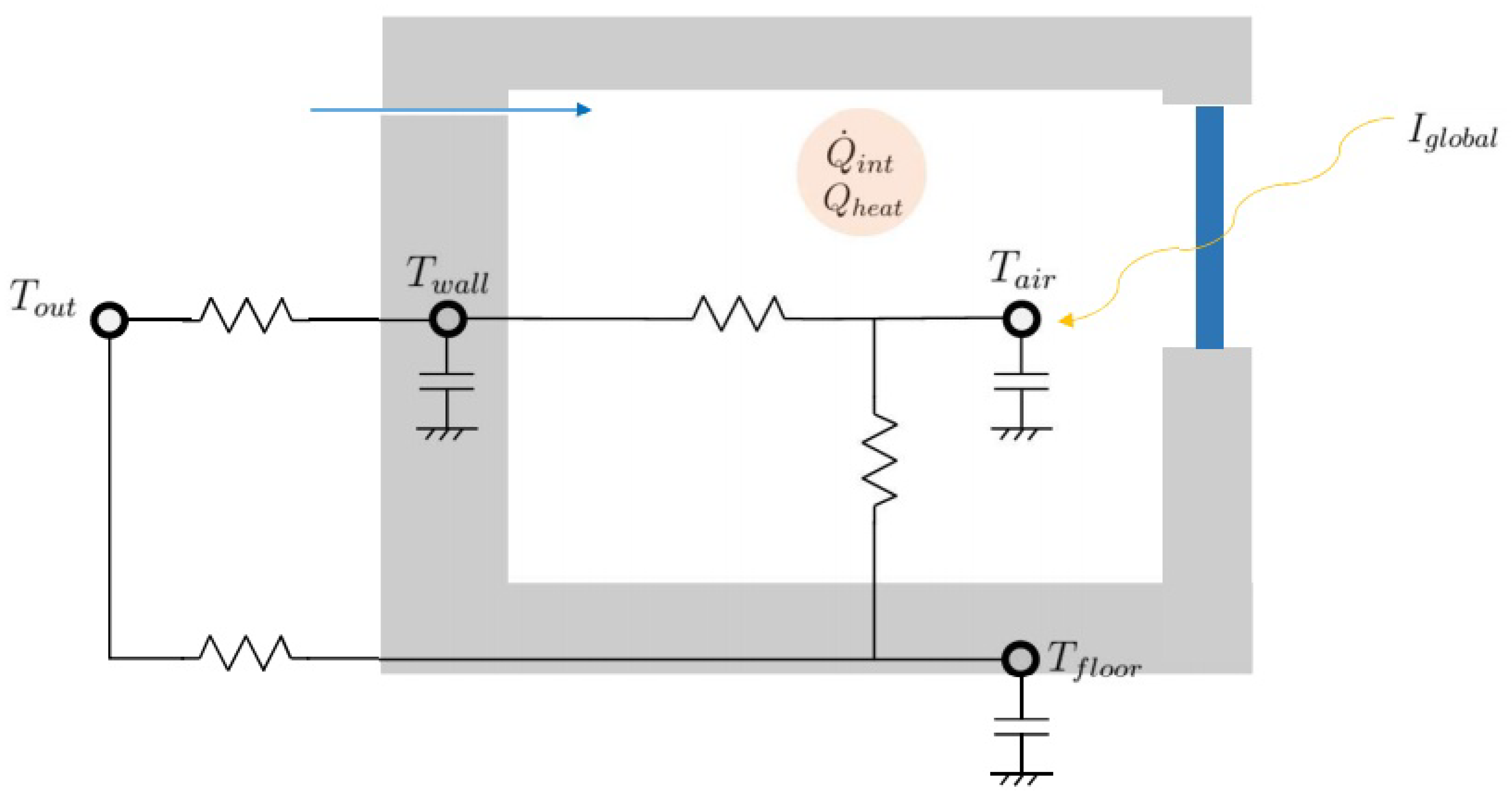
Space Heating

In the case of space heating, the inside air temperature $T^a$, the wall temperature $T^{wl}$ and the floor temperature $T^f$ are the state variables while the outside temperature $T^o$, the solar irradiation I, the internal gains ${\dot{Q}}^i$ and the heating ${\dot{Q}}^h$ are considered as exogenous parameters. The space heating state space model is represented in Figure 1. The system of differential equations is defined based on an equilibrium equation for each temperature node that can be written as:

$$\begin{array}{ccc}{C}_a\frac{d{T}^a}{dt}\hfill & =\hfill & R_{a,wl}(T_t^{wl}-T_t^a)+R_{a,f}(T_t^f-T_t^a)\hfill \\ \hfill & \hfill & +{\dot{m}}_{inf}{c}_{p,a}(T_t^o-T_t^a)+\tau A{I}_t+{\dot{Q}}_t^i+{\dot{Q}}_t^h\hfill \\ \hfill & \hfill & \\ C_{wl}\frac{d{T}^{wl}}{dt}\hfill & =\hfill & R_{a,wl}(T_t^a-T_t^{wl})+R_{wl,o}(T_t^o-T_t^{wl})\hfill \\ \hfill & \hfill & \\ C_f\frac{d{T}^f}{dt}\hfill & =\hfill & R_{a,f}(T_t^a-T_t^f)+R_{f,o}(T_t^o-T_t^f)\hfill \end{array}$$

(6)

where $R_{x,y}$ is the thermal resistance between x and y, ${\dot{m}}_{inf}$ is the mass infiltration rate of outside air, $c_{p,a}$ is the specific thermal capacity of air, $\tau$ is the transmittance of the windows and A the windows area.

In order to get a linear state space model, a linearization of the time derivatives over the desired period is done through the central finite difference method. Linearizing and rearranging the terms, Equation (6) can be written in the same form of Equation (5) thus obtaining explicitly the state space parameters matrices $\mathbf{A}$ and $\mathbf{B}$.

2.2.4. Hot Water Tank

Regarding DHW, the hot water tank is modelled through a state-space model to describe $T^w$ under the hypothesis of isothermal hot water tank.

The influence of the outside temperature $T^o$, the city water temperature $T^{cw}$ and the heating ${\dot{Q}}^h$ is taken into account. The domestic hot water state space model is represented in Figure 2. The equilibrium equation for the hot water tank temperature can be written as:

$$C_w\frac{d{T}^w}{dt}=A{U}_{loss}(T_t^o-T_t^w)+c_{p,w}{\dot{m}}_w(T_t^{cw}-T_t^w)+{\dot{Q}}_t^h$$

(7)

where $C_w$ is the thermal capacity of the water tank, $A{U}_{loss}$ the overall heat transfer coefficient between the inside and outside of the tank, $c_{p,w}$ the specific thermal capacity of water and ${\dot{m}}_w$ the specific hot water consumption determined by the domestic hot water demand.

Rearranging the terms, the state space parameters matrices $\mathbf{A}$ and $\mathbf{B}$ can be determined.

2.2.5. Heating Systems

Heat Pumps

In this work, variable-speed heat pumps are considered. The model describing heat pumps is a linear empirical model based on the ConsomClim method [29] which was obtained by fitting monitoring data relative to a high number of heat pumps types and operating conditions. The same model is used for all the heat pumps, with the only difference of nominal capacity which is determined depending on the insulation level and the supply temperature which is different for space heating and for domestic hot water heating. The nominal characteristics of the heat pumps are the following:

• Outside temperature: 7 °C
• Exhaust temperature: 35 °C
• Capacity: 11.2 kW/14 kW
• COP: 3.95

The heat pumps can operate both in space heating mode or in domestic hot water heating mode but not simultaneously.

The heat pumps’ full load capacity and COP depend on the outside temperature and on the heating system supply temperatures (45 °C for SH and 60 °C for DHW) according to:

$$\begin{array}{ccc}\hfill DT& =& \frac{T_{out}}{T_{su}}-\frac{T_{out,n}}{T_{su,n}}\hfill \\ \hfill CO{P}_{fl}& =& \frac{CO{P}_n}{C_0+C_{1}DT+C_{2}D{T}^2}\hfill \\ \hfill {\dot{Q}}_{fl}& =& \left[D_0+D_1(T_{out}-T_{out,n})\right.\hfill \\ & +& \left.D_2(T_{su}-T_{su,n})\right]{\dot{Q}}_n\hfill \\ \hfill {\dot{W}}_{fl}& =& \frac{{\dot{Q}}_{fl}}{CO{P}_{fl}}\hfill \end{array}$$

(8)

where $C_x$ and $D_x$ are parameters specific to the heat pump design, $T_{su}$ and $T_{su,n}$ are the heating system supply temperatures (effective and nominal), $CO{P}_n$ the nominal performance and ${\dot{Q}}_n$ the nominal heat capacity.

The part-load electrical consumption model of the heat pumps differs in space heating and in water heating. Operating at part load affects the performance (COP) in SH mode but not in DHW mode.

In space heating mode, the heat pump consumption at part load is modelled using a piecewise linear approximation and limited by the consumption at full load performance as described by Equation (9).

$$\begin{array}{c}\begin{array}{c}\hfill W_r\ge 0,77Q_r\end{array}\\ \begin{array}{c}\hfill W_r\ge 0,69+((K_2-K_1)+1,5(1-K_2))(Q_r-0,75)\end{array}\\ \begin{array}{c}\hfill W_r\le Q_r\end{array}\end{array}$$

(9)

where $Q_r=\dot{Q}/{\dot{Q}}_{fl}$ and $W_r=\dot{W}/{\dot{W}}_{fl}$ are respectively the heat and electric part load ratios, while the coefficients $K_1$ and $K_2$ are empirically determined [29]. In addition, the heat pump comprises an additional electric heater for space heating. The capacity of this additional heater is 3 kW. This represent a novel modelling approach which allows to describe the behaviour heat pumps working at partial load in MILP problems in the case of aggregated demand.

In DHW mode, the performance is supposed constant at part load and is equal to the full load performance:

$$\dot{W}=\frac{\dot{Q}}{CO{P}_{fl}}$$

(10)

The total consumption of the heat pumps is the addition of the space heating consumption and the domestic hot water consumption. An additional binary variable y is used to account for the non-simultaneous working of the two modes by limiting their capacities by a fraction y for space heating and $(1-y)$ for domestic hot water.

Water Heaters

The water heaters are electric resistance heaters and provide only domestic hot water heating. Their capacity and performance do not depend on external parameters and they can operate at part load with a constant performance. The coefficient of performance of the water heaters is thus at all time equal to unity.

The water heaters capacity is calculated so that they are able to maintain the tank temperature its minimum allowed value

$${\dot{Q}}^d=ma{x}_h\left\{\dot{Q}:\Delta T_h{\parallel }_{T_{w,min}}=0\right\}$$

(11)

and within the limited range $\left[{\dot{Q}}_{min},{\dot{Q}}_{max}\right]=\left[1\mathrm{kW},4\mathrm{kW}\right]$.

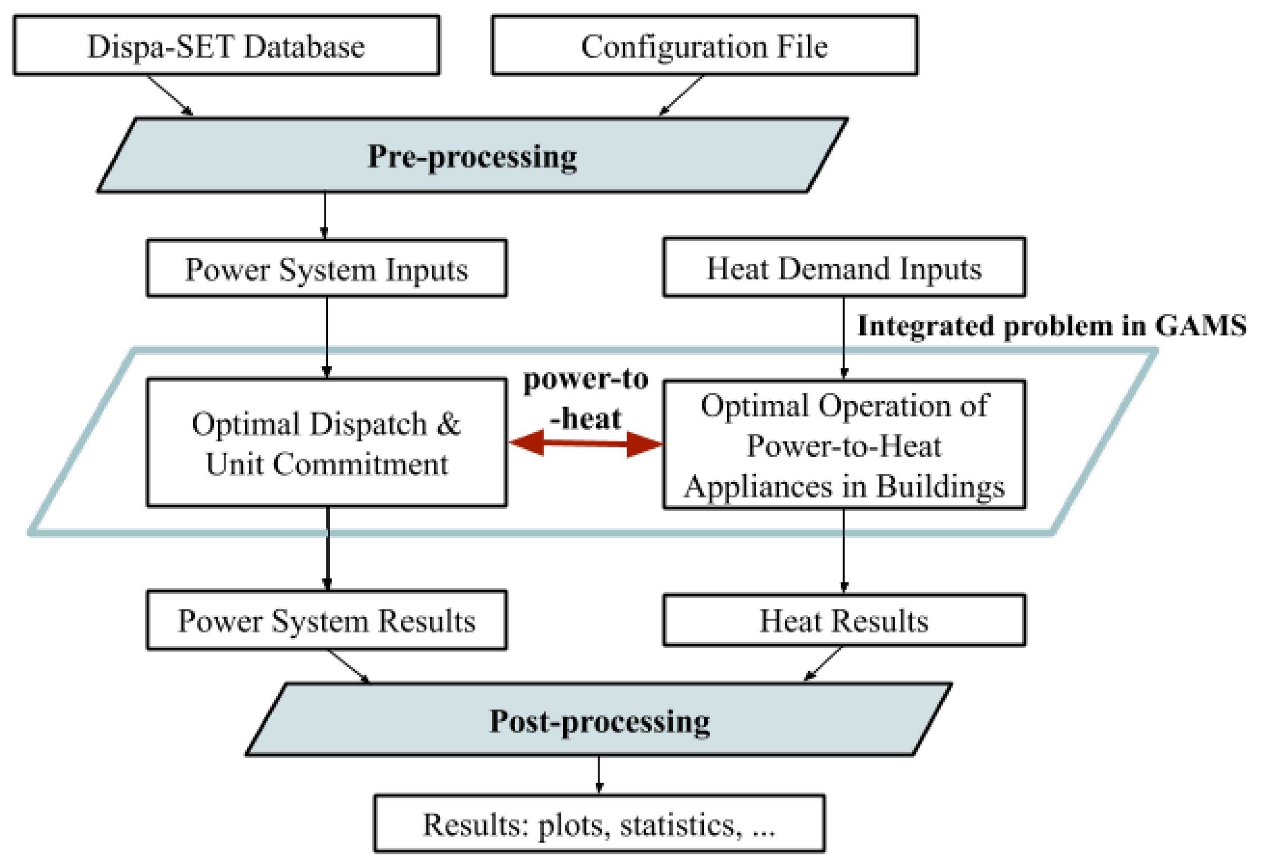
2.3. Integrated Model

The integrated model presented in this work is obtained from the integration of the demand side model (space and water heating) introduced in Section 2.2 into the existing supply side model Dispa-SET for the power system that was presented in Section 2.1. The mathematical program is formulated as follows:

$$\begin{array}{cccc}\hfill min& \hfill & & \mathit{System}\mathit{cost}\hfill \\ \hfill s.t.& \hfill & & \mathit{supply}-\mathit{demand}\mathit{balance}\hfill \\ \hfill & \hfill & & \mathit{supply}\mathit{side}\mathit{constraints}\hfill \\ \hfill & \hfill & & \mathit{demand}\mathit{side}\mathit{constraints}\hfill \end{array}$$

(12)

A simple scheme representing the main modules of the integrated model is available in Figure 3.

The conjunction between the two models is realized by introducing power-to-heat options to the system (heat pumps and electric water heaters) and by the add of the thermal demand to Equation (2). Equation (13) represents the demand-side balance constraint for the integrated model.

$$\begin{array}{c}\begin{array}{c}\hfill \sum _u\left({\mathit{P}}_{u,i}·{\mathit{Location}}_{u,n}\right)+\sum _l\left({\mathit{Flow}}_{l,i}·{\mathit{LineNode}}_{l,n}\right)\end{array}\\ \begin{array}{c}\hfill ={\mathit{Demand}}_{n,i}+{\mathit{Demand}}_{HeatDevices,n,i}+\sum _r\left({\mathit{StorageInput}}_{s,i}·{\mathit{Location}}_{s,n}\right)\end{array}\\ \begin{array}{c}\hfill -{\mathit{ShedLoad}}_{n,i}\end{array}\end{array}$$

(13)

where ${Demand}_{HeatDevices,n,i}$ is the electric load associated to the users thermal demand. This latter is alternatively defined as an exogenous variable (when the thermal units are considered non-flexible) or as an optimization variable (in the case of flexible heat pumps or electric water heaters).

All simulations are performed for a whole year with a time step of 1 hour. To reduce the computational burden, the problem was split into smaller optimization problems that are run recursively throughout the year. In order to avoid end-of-horizon artefacts (such as emptying of the hydro reservoirs) with this rolling horizon approach, a look-ahead period is used but discarded for the following optimization horizon [30]. In addition, the optimization is partially relaxed: the solution has to be close enough to the optimum relaxed (linear) solution obtained. An optimality criterion is fixed as the distance between the best relaxed solution and the MILP solution. Here, the optimality gap criterion is set at 1%.

The constraints of the system are represented by the sum of all the demand side and supply side model constraints illustrated in the previous sections, while the objective function is the total system cost (Equation (1)).

3. Simulations and Results

In this section, the analyzed scenarios are described. Then, performance indicators are defined and the results are finally presented and discussed. It is important to note that all simulations were performed under a “perfect forecast” assumption: all the parameters of the model were considered to be predicted with no error for the analyzed period of time. For this reason, the benefits of the flexible heating devices assessed in this work have to be considered as an upper bound of the benefits of residential DR, limited in practice by forecast errors and sub-optimal control.

3.1. Scenarios

Starting from the base case scenario, a certain number of simulations was performed in order to assess the potential of heat pumps and resistance water heaters in terms of flexibility, RES integration and total system costs at country level. The dependency of these results on the power system configuration was also analyzed. The base case scenario, including the characteristics of the capacity mix, of the system costs and of the electric demand, was defined as the one provided by Dispa-SET for Belgium in 2015 with the total installed capacity composed for around one third by nuclear power, one third by gas-fired units and one quarter from variable renewable sources (16% sun and 10% wind). The other scenarios were obtained through variations both on the demand (diffusion of electric heating technologies) and supply side (variations in the capacity mix) of the system and can be summed up as described in

Table 1. Parametric analysis scenarios.

Heating technology	HP—WH
Number of flexible units	0—0.2—0.4—0.6—0.8—1 M
Renewable capacity	R1—R2—R3
Non-renewable capacity	Nuclear power (non-flexible)—gas-fired units (flexible)

. Simulations were performed for six different supply-side configurations: the renewable capacity was varied from one to three times the current renewable capacity (R1, R2, R3). Moreover, for the power system configuration, two possibilities were evaluated considering the current scenario, which included a relevant share of nuclear power plants, and an alternative configuration with nuclear capacity substituted by gas-fired units, which are typically more flexible in their operations.

On the demand-side, simulations included a sensitivity analysis on the number of installed electric heating units (heat pumps and water heaters alternatively) which was varied between zero (non-flexible demand) to one million units, with the national building stock accounting for a total of 5.6 million dwellings based on the latest data available [31].

Moreover, additional scenarios were analyzed to compare the performances of the thermal storage capacity achievable with heating-electricity sector coupling solutions with the one offered by the existing hydro pumped storage units. To this aim, a new base case scenario was formulated including no storage units. This latter was compared with simulations including alternatively hydro pumped storage (with an installed capacity equal to the one already installed), flexible heat pumps (1 M) and flexible water heaters (1 M). The main features of the simulations are described in

Table 2. Storage units comparison scenarios.

Storage technology	No storage units—HPHS (1308MW—HP (1 M)—WH (1 M)
Renewable capacity	R3
Non-renewavble capacity	Nuclear power (non-flexible)

.

3.2. Performance Indicators

The main indicators employed for the comparison of different scenarios were the following:

• Energy system operational costs
• Total load variation
• Curtailment
• Roundtrip storage efficiency (ratio of the useful energy to the total energy stored)

All the indicators were computed on the basis of 1 year simulations and were descriptive of the Belgian energy system.

3.3. Results

3.3.1. Base Case Scenario

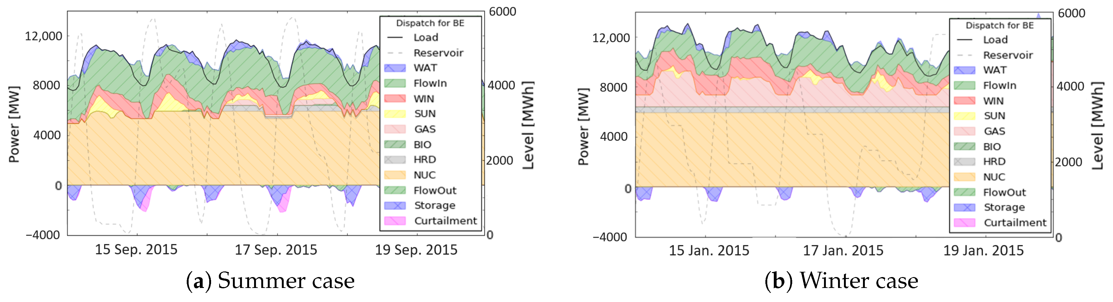
In the base case scenario the share of renewables was equal to 11.9% with 1.2% curtailment.

Figure 4a shows the optimal dispatch in some summer days which were most critical for curtailment. It has to be noted that in the base case scenario, curtailment did not arise from an excess in renewable availability compared to the demand but was due to the non-flexibility of the nuclear power plants. Base load units were unable to follow the residual load variations induced by renewable generation. This explains the fact that some curtailment took place in night time due to the reduced load in these hours. In the base case scenario, pumped hydro storage and other storage units provided most of the flexibility to the system. These units appeared to absorb a significant part of the excess energy and thereby reduce curtailment.

Figure 4b shows a typical winter day. Significant differences between summer and winter were observed. First, no curtailment occurred. Then, the generation of nuclear and coal units was more stable. Finally there was a significant increase in non-nuclear conventional generation in particular gas fired power plants due to the higher demand (between 1 and 2 GW more then in summer). These effects arose without significant reduction in variable renewable generation. This load increase allowed low-cost non-flexible units like nuclear power plants and coal units to work at full load. Flexibility was provided mainly by gas fired combined cycle power plants.

3.3.2. Water Heater Scenarios

In the following scenarios, the impact on the energy system deriving from the diffusion of flexible water heaters was analyzed. Contrary to heat pumps, these units only provided DHW (cfr Section 2).

Operational Cost

The total operational costs of the system with non-flexible heating devices is shown in

Table 3. Total operational cost for the different base-case scenarios [M€].

	Nuclear Power (Non-Flexible)	Gas-Fired Units (Flexible)
R1	711	2362
R2	544	2026
R3	457	1705

. It can be seen that an increase in the renewable capacity made the operational costs decrease significantly. On the other hand, the shift from nuclear power to gas-fired units led to more flexibility but also to higher operational costs.

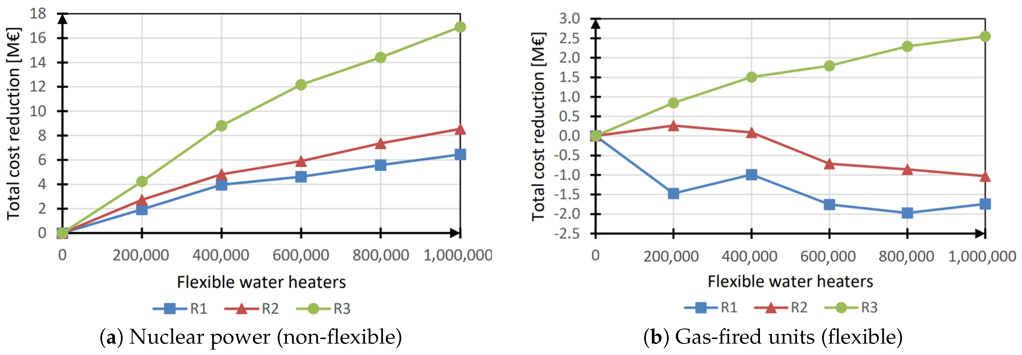
Figure 5 shows the operational costs reduction which could be obtained through the progressive diffusion of flexible water heaters.

In the system configuration including nuclear power, Figure 5a shows that the more water heaters were made flexible, the higher the benefit in cost reduction. Moreover, increasing the renewable capacity also increased this cost reduction.

A higher renewables penetration increased the system’s need for flexibility as well as the savings obtainable by flexible heaters diffusion. As a general trend, the increase in cost benefit seemed to follow a sub-linear trend with respect to the diffusion of flexible units; in fact, when water heaters’ flexibility was unlocked, the system flexibility increased and its flexibility need decreased, reducing the marginal benefit linked to an additional flexible unit. Saturation was however not reached in these simulations (i.e., additional flexible water heaters always benefited the operational cost).

In the case of shift from nuclear to gas-fired units, Figure 5b shows results comprised between €2 million of cost increase (R1) and €2.5 million of potential savings (R3). However, the obtained results fell below the solver precision and could therefore not be considered as significant. In those scenarios, because of the flexible resources already present in the system, the spread of flexible electric heaters did not have a significant influence on the system costs.

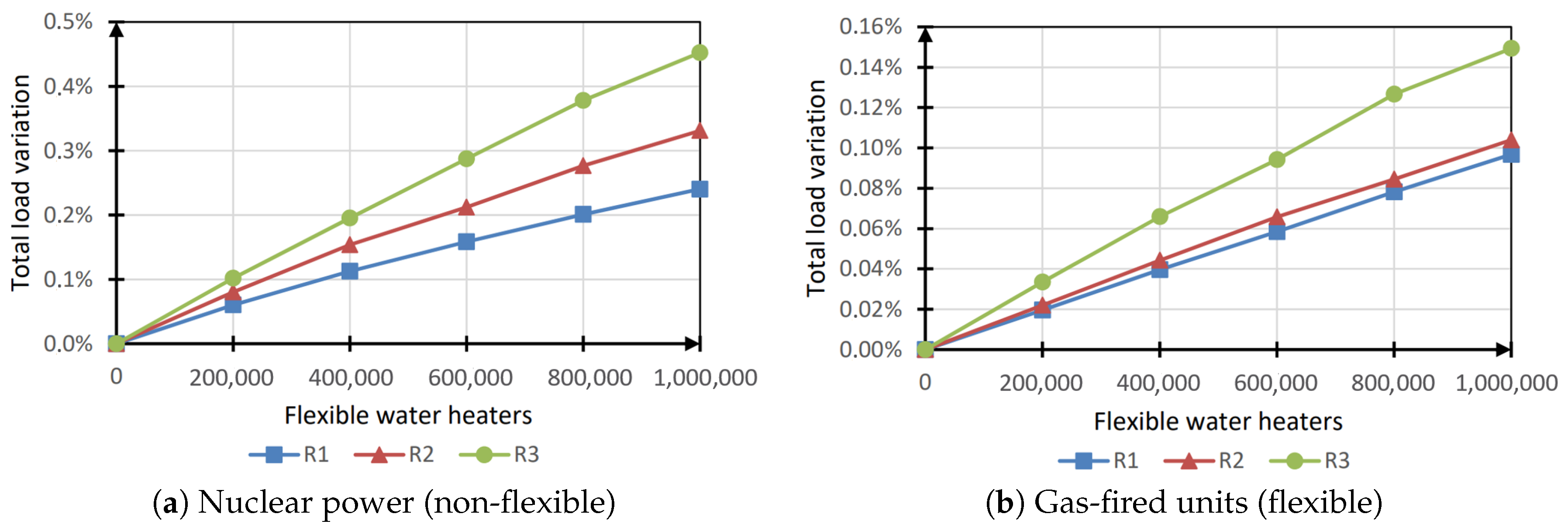
Total Load Variation

The load variation caused by the flexibility activation of the water heaters is shown in Figure 6. The penetration of flexible devices seemed to lead to an increase in the total load (mainly caused by the thermal losses of the thermal storage); however, the observed variations could not be considered relevant being lower then the solver precision. Therefore, it can be concluded that the activation of flexible water heaters did not significantly increase the total electricity load.

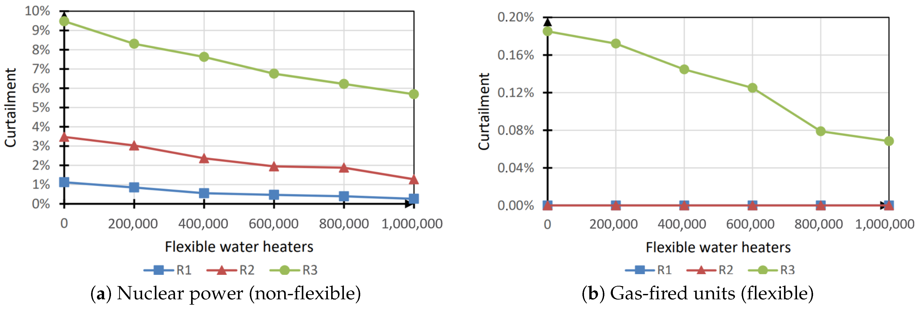
Curtailment

Figure 7 shows the curtailment variation when flexible water heaters were added, demonstrating, in the low-flexibility case, that it decreased significantly with the introduction of more flexible devices. The variation increased with the increasing penetration of renewables in the system. In the high flexibility case (shift from nuclear to gas) the system had enough flexibility to cope with the intermittency of renewables and the introduction of flexible electric heaters had a negligible effect on the total curtailment.

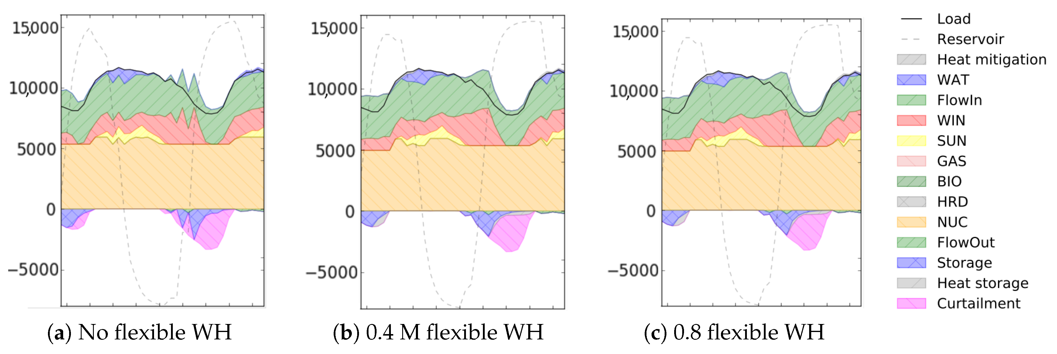
Figure 8 shows a typical day where curtailment occurred (R2—nuclear power configuration) for three penetration levels of flexible water heaters.

When 0.4 M flexible heaters were introduced, thermal storage was able to offset all the curtailed power of the first period and a part of the second period. Increasing the number of flexible heaters to 0.8 million further reduced curtailment, but without completely offsetting it.

3.3.3. Heat Pumps Scenarios

In this section, the results for flexible heat pumps scenarios are discussed and compared to the results of the electric heater case.

Operational Cost

The total operational cost reduction is shown in Figure 9. Compared with the water heaters cases, the cost reduction was larger and became more significant with the shift from nuclear to gas-fired units.

When heat pumps flexibility was “activated”, cost reduction occurred for two reasons: the increase in flexibility (like for water heaters) and the heat pump consumption reduction thanks to an improved control strategy which optimized its part-load performance over time.

In the gas-fired units configuration, the flexibility provided by the heating systems had no significant effect on the total cost. In these cases, the cost reduction observed was entirely due to the consumption reduction. This consumption reduction remained constant for different renewable capacities installed.

For the nuclear power case, cost reduction became significant and the total cost reduction was more important.

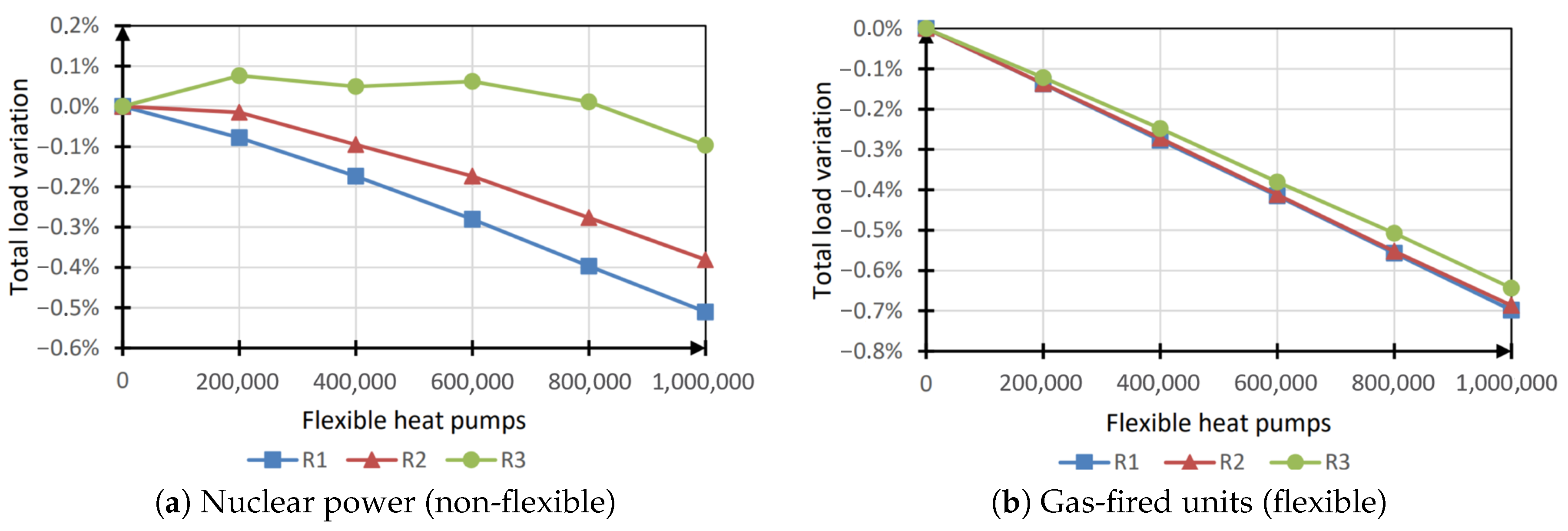
Total Load Variation

Figure 10a represents the obtained results for the total load variation in the case of flexible heat pumps. As for the water heaters simulations, the total power consumption was not significantly affected by the introduction of flexible heat pumps: in both nuclear and gas-fires units case, the variation was lower than the simulation accuracy (equal to 1%).

3.4. Comparison between Storage Technologies

In this paragraph, the storage and overall system performances of flexible water heaters and heat pumps are compared with the ones offered by existing hydro pumped storage units. To this aim, four simulations were performed, as described in Table 2. The main results are resumed in

Table 4. Storage technologies performances.

	HPHS	HP	WH
Installed Storage Capacity [MW]	5886	24,848	3489
Avoided curtailment [MWh]	1,684,580	1,462,927	1,046,394
Specific avoided curtailment [MWh]	286.2	58.9	299.9
Total stored energy [MWh/MW]	1,863,084	6,422,305	1,319,002
Specific stored energy [MWh/MW]	316.5	258.5	378.0
Storage peak [%]	100	100	100
Roundrip efficiency [%]	0.74	0.90	0.68

.

Avoided curtailment is expressed with respect to the base case scenario, which includes an amount of curtailed power equal to 2,995,154 MWh.

Results showed that pumped hydro storage (HPHS) and flexible water heaters were the most performing technologies in terms of specific avoided curtailment (expressed as the ratio between avoided curtailment and virtual/installed energy storage capacity). Roundtrip efficiency was higher in the case of heat pumps, while the flexible water heaters’ storage roundtrip efficiency was similar to the one of hydro pumped storage units.

In addition to the scenarios described, more simulations were performed in order to find the equivalent installed capacity of HPHS able to provide the same results of flexible thermal units in terms of avoided curtailment. Results showed that 3105 MWh of HPHS storage capacity would provide the same curtailment reduction as 1 M flexible WH scenarios, while for the case of flexible HP, 4761 MWh would be necessary.

In general, results proved the effectiveness of heating-electricity sector coupling technologies in capturing the inherent thermal storage potential of the thermal device itself and of the building envelope, ensuring in this way a valid alternative to traditional energy storage units as pumped hydro storage.

Nevertheless, even if the flexibility potential of electric heating technologies came with no additional investment costs, its practical exploitation required great effort in terms of data forecasting and management of the service compared to more traditional flexibility sources like HPHS.

4. Conclusions

This paper presents an innovative modelling framework in which building and DHW models are directly integrated within a well-established unit commitment and optimal dispatch model.

The demand side heat model is calibrated for the case of the current Belgian building stock. The demand for heating is linked to the electricity demand through accurate state space models and electric heating systems models for flexible resistance water heaters and flexible air-to-water heat pumps. The combined model allows optimizing both the operation of the power system and the smart management of the flexible units. The optimization if performed under a perfect foresight hypothesis and should therefore be considered as representative of an upper limit of the available flexible resources through demand response.

A parametric analysis was performed assessing the influence of the flexible devices penetration, the renewable capacity and the composition of the capacity mix. Results show that significant benefits can be achieved with demand response management. Operational cost benefits up to €16 per water heater and €35 per heat pump are assessed. Thermal storage has the potential to offset up to 1 TWh of curtailment with 1 million electric heating systems (1 MWh of curtailment reduction per electric device) over the optimization period when the flexibility needs are the most important (high renewable capacity and nuclear power configuration). It is important to note that these benefits are reduced significantly when the shift from nuclear to gas-fired units (more flexible) occurs thanks to a higher ability of the system to follow renewables generation.

It can therefore be concluded that demand response applied to flexible electric heating devices offers significant flexibility resource to the system. This is especially true if more renewables are added to the system and if the power plant fleet is relatively non-flexible. The results highlight the importance of considering not only the demand-side and the renewables penetration in the system, but also the existing capacity mix and its characteristics when dealing with the flexibility potential offered by demand response. This can only be achieved through integrated models, and thereby justify ex post the relevance of the proposed modelling framework.