Abstract
Determination of local heat transfer coefficient at the interface of channel wall and fluid was the main goal of this experimental study in microchannel flow boiling domain. Flow boiling heat transfer to DI-water in a single microchannel with a rectangular cross section was experimentally investigated. The rectangular cross section dimensions of the experimented microchannel were 1050 m × 500 m and 1500 m × 500 m. Experiments under conditions of boiling were performed in a test setup, which allows the optical and local impedance measurements of the fluids by mass fluxes of 22.1 to 118.8 and heat fluxes in the range of 14.7 to 116.54 . The effect of the mass flux, heat flux, and flow pattern on flow boiling local heat transfer coefficient and pressure drop were investigated. Experimental data compared to existing correlations indicated no single correlation of good predictive value. This was concluded to be the case due to the instability of flow conditions on one hand and the variation of the flow regimes over the experimental conditions on the other hand. The results from the local impedance measurements in correlation to the optical measurements shows the flow regime variation at the experimental conditions. From these measurements, useful parameters for use in models on boiling like the 3-zone model were shown. It was shown that the sensing method can shed a precise light on unknown features locally in slug flow such as residence time of each phases, bubble frequency, and duty cycle.
1. Introduction
Flow boiling in microchannels is considered as an effective method for heat removal and energy transport in chemical microreactors and heat exchangers [1]. Thus, understanding flow boiling heat transfer in microchannels is an important concern for a wide variety of applications such as electronics cooling [2]. Many experimental and theoretical studies in the literature aimed at understanding the physics and underlying heat transfer mechanisms behind the boiling flow in a microchannel with two general attitudes [2,3,4]. First, some researchers tried to come up with new correlations and prediction methods for both boiling heat transfer coefficient and two phase pressure drop [5,6]. Second, there have been efforts in order to analyze the physics behind the microchannel boiling by resolving high resolution temperature information in controlled situations and proposing a physical model that describes the heat transfer during boiling [4,7,8]. Despite the wide variety of published research works, due to the complex nature of the topic there is still space for improvement and issues to study on heat transfer mechanisms, pressure drop characteristics, and two-phase flow instabilities regarding boiling in microchannels [2,6,9]. In addition, recently different methods have been proposed by researchers to enhance the stability of flow boiling performance such as surface modification, thermal equilibrium improvement, disturbance intensification, and nucleation enhancement [10,11,12].
The vast majority of researchers focused on the influence of operating parameters on the heat transfer of microchannel flow boiling such as working fluids, aspect ratio, and cross-sectional shapes of microchannel as well as surface roughness [13,14,15]. Consequently, many different empirical correlations were developed in order to predict the heat transfer coefficient concerning boiling liquids in a mini- or microchannel. However, there is no universal agreement between these models due to the fact that experimentations have been performed over a wide range of different operation parameters and experimental conditions. Therefore, the extrapolation of available correlations to other experimental conditions may show discrepancies [16,17]. In addition, most of the existing correlations do not have satisfactory accuracy to predict critical heat flux, heat transfer coefficient, and flow pattern transition boundaries [2]. The researchers found that developing flow boiling heat transfer prediction models based on mechanistic distinction criteria is more practical and effective [16,18,19]. Therefore, detailed knowledge of the system is still necessary to understand the specific flow boiling mechanism in order to develop a predictive model [16].
It has been illustrated that there are essential links between flow boiling mechanisms and flow regimes. According to the observed flow patterns in literature, four different criteria were reported for heat transfer mechanism in microchannel boiling flow. In the first criterion, the nucleate boiling heat transfer is dominant. In this case, bubbly flow regime appears with low vapor quality where the heat transfer coefficient is strongly influenced by heat flux. The effect of mass flux and vapor quality on heat transfer coefficient is very low [20]. The second criterion is based on mixture of nucleate boiling and convective boiling heat transfer. In this case both mechanisms take place simultaneously in bubbly and slug flow regimes respectively which alternate in time and space. Here the local heat transfer is strongly affected by heat flux and vapor quality but weakly affected by mass flux [21,22]. Thirdly, the convective boiling heat transfer is dominant. Forced convection boiling occurs in saturated region of the microchannel with high vapor quality. Heat transfer is increased by convective mechanism and nucleation process is almost restrained. The heat transfer coefficient was found to be independent of the heat flux while it increased with an increase in the mass flux and decreased with an increase in the vapor quality. The convective evaporation was reported as the dominant mechanism for annular and semi annular pattern [23,24]. The fourth mechanism is dominant thin film evaporation heat transfer. It was clarified by researchers that the major heat transfer mechanism for elongated bubble and annular flow pattern is due to thin film layer evaporation between the vapor core and the heated wall surface [25,26,27]. Thome and Consolini [28] report that the heat transfer coefficient is not only influenced by heat flux through dominant nucleate boiling mechanism but also is dependent on thin film evaporation and bubble frequency. They experimentally determined a trend in the local heat transfer coefficient versus local vapor quality and the measured trend during liquid film evaporation does not show the expected increase with quality. In general, local heat transfer measurement in combination with flow visualization can be beneficial to recognize the dominant flow boiling heat transfer mechanism in microchannels [2].
Several boiling heat transfer prediction models were developed to relate the heat transfer fundamental mechanisms with flow regimes and vapor bubble dynamics practically [18,29,30]. The main methods in experimental boiling flow analysis in microchannels are proposed to estimate or measure local wall temperature, channel pressure drop and visual detect flow patterns. A model for the estimation of the heat transfer coefficient is consequently established. In this regard, Jagirdar and Lee [31] investigated the transient local heat transfer coefficient at different locations in a single mini rectangular channel during subcooled flow boiling. They observed variation of the heat transfer coefficient over a given location due to passing of different flow patterns. An increase of the local heat transfer coefficient was observed due to the passing of bubbles with evaporating thin films. Bigham and Moghaddam [7] also reported similar observations for flow boiling experiments in single microchannel featuring nanostructured elements. Since the local fluid temperature, wall temperature, or heat flux measurement is challenging for the calculation of a local heat transfer coefficient, it is typical to use data reduction methods to calculate local surface temperature [32,33].
As outlined above, there are multiple existing experimental studies on the water boiling in metal or silicon microchannels over a limited range of operating conditions. Large uncertainties have been found in most of the reported experimental data [2,6]. The developed heat transfer correlations based on these experimental studies are not universally applicable. Therefore, it is necessary to refine the experimental procedures, measuring instrumentation, and measuring techniques to obtain more reliable data. It is necessary to reach an appropriate data reduction method for each specific test setup. From the viewpoint of application, heat sinks comprising rectangular microchannels, machined in metal plates, such as stainless steel, copper, or Aluminum are highly applicable due to the high heat dissipation capability and the ease of manufacturing. However, a good prediction of the heat transfer properties has to be done. Using low-pressure water in microchannel boiling process has been reported as an attractive coolant for chipping cooling applications due to its high latent heat [34].
In the current work, we report the analysis of experimental data on the local heat transfer of water evaporation in a single stainless steel rectangular microchannel. In our previously published work, the proof of principle for determining the local flow regime by using impedance sensing has been shown [35] besides the application of analyzing slug flow [36]. As discussed above, the flow regime is vitally important for the heat transfer mechanism and thus for the estimation of the heat transfer coefficient. The objective of the present investigation is to further study the characteristics of microchannel flow boiling by correlating the differences in the measured local heat transfer coefficients. The effect of mass flux and heat flux on the local evaporation heat transfer are investigated and presented. We aim to develop a new technology based on capacitive sensing that is able to contribute to cooling system developments. In the last part, the possibilities of using local electrical sensing as feed-in for refining heat transfer models is presented.
2. Experimental Setup
Figure 1 presents the schematic diagram of the experimental apparatus used in this study and previously described in [35]. The experimental setup consists of a Pyrex reservoir to store deionized water. DI-water was pumped at a constant flow rate and degassed through the flow loop using a HNP mzr-7205 micro gear pump with constant flow rate. The flow rate was measured using a Sensirion SLQ-QT500 flow meter. Swagelok Stainless Steel fittings and Festo push in connectors were used to construct the flow loop. Figure 2 represents the exploded structure of the test device which was used [35,36]. As it is shown in the exploded view of the test section in Figure 2, the test section consists of a housing(1), a glass cover lid(5), a heater block(2) equipped with 6 DC electrical heater cartridges(8), and a stainless steel microchannel plate(4). The housing body, lid, and heater block were made from Aluminum. The Aluminum lid(6) presses the cover glass to the O-rings on the microchannel for sealing purposes. In order to facilitate flow visualization, perform impedance measurements, and seal the microchannel, a Pyrex lid(5) with 2 mm thickness and patterned sensing elements is fabricated in a cleanroom. The glass lid has patterned indium tin oxide elements which are visually transparent and conductive. Therefore, simultaneous electrical sensing and visual inspection were possible in each sensor location. The details of the glass lid fabrication method were previously explained in [37]. The contacting of the probes was done using spring probes(11). The housing part has the inlet and outlet with assembled pressure and temperature sensing probe locations. The PEEK parts (9 & 10) under the bottom part of housing were considering as electrical and heating insulators to reduce the heat loss to the ambient and as holders to keep whole the test section in a stable position. The microchannels were fabricated using CNC machining on the surface of a stainless steel plate with plate thickness of 5 . Two o-ring grooves are machined on the surface of microchannel plate to provide sealing around the channel and make an appropriate area for the glass to sit on. Six small holes were drilled in side wall of channel plate to with the 0.5 distance underneath of microchannel wall for inserting thermocouples to measure the temperature along of the channel. The highspeed videos that are recording in this work were acquired by highspeed camera Phantom VEO 410L manufactured by Vision research. The measurement device that was used for impedance measurements was MFIA impedance analyzer by Zurich Instruments. At the beginning of each measurement, the camera receives a trigger signal from the measurement device for a precise time synchronization.
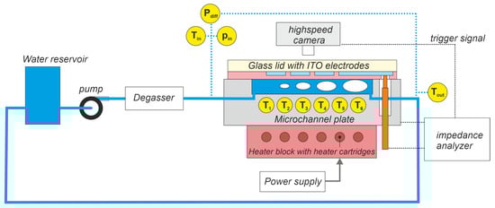
Figure 1.
Schematic of experimental set-up.
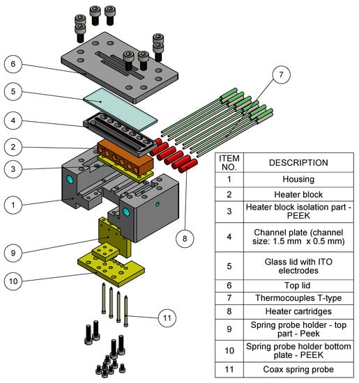
Figure 2.
Exploded view of test device assembly.
Regarding temperature monitoring, in the whole test apparatus 16 T-type (Copper/Constantan) thermocouples are located. The exact location of the implemented thermocouples are shown in Figure 3. Temperature measurement on the flow was established before entry to the test section (), after the exiting test section (), at the inlet () and outlet () of the channel, at six positions underneath the channel wall in the plate (), and at six locations in the heater block (). The experimental data was recorded in time transient conditions and further averaged to obtain stable values. The data was used to analyze the thermal balance of the test setup in the data reduction step (see below). The thermocouples data was read out in approximately 1 Hz sampling rate by two data logger devices from Pico Technology TC-08 with built-in ambient temperature readout. The ambient temperature read out was used to calculate heat loss more precisely for the tests that were performed on different days. The DI-water was degassed before flowing into the test device. The heat flux was applied by DC electrical heaters(8) to heating blocks. The heat flux was increased gradually to obtain a recognized stable operating condition during either a single-phase or a boiling flow through the experiments. Single-phase flow experiments were conducted to estimate the heat loss. During the single-phase flow test, the fluid temperature was allowed to increase without reaching the onset of boiling.
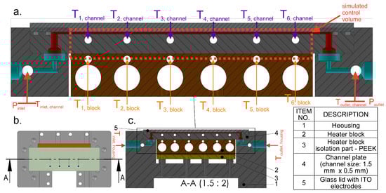
Figure 3.
Thermal path with implemented sensors of the boiling liquid in the housing. Light blue is the liquid path inside the housing and red is liquid path inside the channel plate. (a). Cropped zoom of the cross section with temperature sensors in the channel plate, heater block, and housing. (b). Top view of the housing assembly with heater block, channel plate, and glass lid. (c). A-A cross section of the housing assembly.
The uncertainties of the measured values were directly supplied from the manufacturers’ specification sheets. Table 1 presents the ranges of the experimental variables. The pressure sensor was a KELLER AG PRD–33X model. Pressure sensing in the experiments was performed by a sensor that measures differential pressure and inlet pressure at the same time. The measurement accuracy for the differential pressure sensor is 35 and that of the inlet pressure sensor is 40 (0.1% full scale). Temperature measurements were performed by temperature data logger with the uncertainties of ±C for the T-type thermocouples. The uncertainty associated with the voltage and current applied to the heater cartridges was smaller than mV and respectively [38].

Table 1.
Experimental parameters and uncertainties [35,38,39].
For each experimental run, input power and flow rate were set as input conditions. An example of the acquired raw temperature and pressure data from the test setup for each experimental condition is shown in Figure 4. In each experiment, the waiting time was set to long enough (minimum 25 min) until the signal of the thermocouples reach constant and stable values so that we can consider the situation steady state in respect to data reduction and use the averaged values for each sensor. As Figure 4a demonstrates, temperature measurements along the heater block can be considered uniform and Figure 4b shows channel temperature sensors information vs. time. The observation was qualitatively consistent for all experiments. The averaged block and channel plate temperature along the channel plate referenced to the inlet point location are shown in Figure 4c. Figure 4d,e show pressure drop measurements in time and frequency domain respectively for a two phase experiment. Figure 4e displays that pressure flow oscillations have a peak around 4 Hz. This is a good example of unstable conditions in pressure drop in flow boiling.
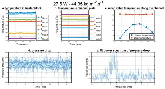
Figure 4.
Example of raw data using a heating power of 25 and a flow of 1 mL/min (22.17 ) water acquired by test setup. (a). Time domain recorded temperatures of thermocouples located in heater block. (b). Time domain recorded temperatures of thermocouples located in channel block. (c). Mean value of the recorded temperature in each sensor. (d). Time domain recorded pressure drop in the channel. (e). Power spectrum of the Fast Fourier Transformation of pressure drop.
3. Data Reduction
In order to obtain a meaningful analysis of the phenomena from the acquired experimental data, it is necessary to relate the measured data to the actual effects. For pressure drop that means to subtract the pressure drops which are not part of the flow in the channel, in order to deduct corner pressure drops caused by the 90 degrees bends, as well as expansion and contraction pressure drops (Equation (1a,b)). The flow goes via four bends, the pressure drop for those was given by equation Equation (2a). Additionally, there was a certain pressure drop through the expansion of the fluid, which was given by Equation (2b).
In Equation (1b), is the pressure drop at each of the corners that were in the path between two sensor locations (see Figure 3). The corner pressure drop was calculated using Equation (2a) with [6,40]. The expansion and contraction pressure drops are calculated by Equation (2b) with and [14,40,41].
The fanning friction factor of the channel for single phase experiments is calculated using Equation (3) based on measured channel pressure drop.
In order to calculate effective heat that enters the channel footprint, a heat loss correlation was developed for the test setup based on single phase experiments tailored to each flow rate. The experimental data for these correlations were acquired by applying lower power than necessary for evaporation and same flow rate for each channel. Heat loss calculation has been done using Equation (4a). was calculated using Equation (4b), thereby the influence of ambient temperature variations in the lab is considered and compensated. For each flow, acquired a and b factors from single phase experiments were used to calculate two phase heat loss. a and b are model parameters in a linear description of heat flow from the heaters to the ambient based on temperature difference. The average temperature value of block 3 and block 4 temperature sensors were picked since these sensors were located in the middle of the channel.
By applying the energy balance equation on our control volume, the energy entered to the channel is derived by Equation (5a). After the deduction of heat loss from total applied heat by power supply (Equation (5b)), the heat entering to the channel was calculated using the heat balance (Equation (5a)). Figure 5 illustrates the schematic of microchannel, the used coordinates in the equations (z is along the flow), and heat transfer surfaces between the channel plate and flowing liquid. denotes the energy absorbed by the liquid in the path between entering the housing and entering to channel and is described by Equation (5c). On the other hand, the liquid exits the channel at saturation temperature and the temperature drops until it reaches the sensing point. In Equation (5d), if the temperature measured by sensor is higher than the saturation temperature, it is assumed that 60% of vapor exiting the channel condenses until it reaches the end of the control volume. This energy is denoted by which is based on latent heat at saturation temperature.
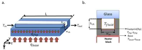
Figure 5.
Schematic of the single microchannel evaporator. (a) isometric view of channel plate. (b) cross section of the channel plate.
The global heat flux at the channel is calculated by dividing energy that enters into the channel to effective hot surfaces (Equation (6)). All heat to the liquid was supplied via the footprint surface that was metallic and encompassed three sides of the channel. The glass lid on top did not heat the liquid. In Equation (7), L is channel length, h was channel height that is 0.5 in both experimented channels and w is channel width.
In order to estimate the local heat flux along the channel, the temperature gradient between heater block’s temperatures and channel plate’s temperatures was used. A third degree interpolation between the 6 point temperature measurements in the heater block and another interpolation for 6 point temperature measurements at the channel plate were performed. Therefore, the normalized gradient of the temperature at each z was multiplied to (Equation (8)).
Consequently, the footprint temperature is derived from Equation (9) and fluid temperature along the channel was determined by Equation (10). b is the metal thickness between channel plate temperature sensor locations and channel wall which is 0.5 mm. In Equation (10), cannot rise above saturation temperature; it is equal to saturation temperature since the absorbed heat is consumed for phase transfer.
The local heat transfer coefficient at footprint is expressed by Equation (11). In Equation (11), is set to saturation temperature for two phase flow region.
With the knowledge of the heat flux towards the footprint, the boiling front and consequently the local vapor quality and void fraction were determined using Equations (12) and (13).
The heat transfer coefficient in the boiling region of the channel is calculated using Equation (14) [6]. In this equation, is logarithmic mean temperature difference between minimum and maximum temperature of channel plate and liquid inlet and saturation temperature respectively.
4. Results and Discussions
Experimental results presented in this section were performed at about atmospheric system pressure both for single phase and two phase experiments. Two different plates with channels measuring 750 m (1.5 mm × 0.5 mm) and 677 m (1.050 mm × 0.5 mm) were used for these experiments. The absolute mean error value for experimental results compared with available correlations is calculated based on Equation (15).
4.1. Single Phase Pressure Drop Validation
Prior to two phase experiments, single phase experiments in a room temperature condition were conducted to ensure that the test rig performed properly and measurement devices such as pressure sensors performed with reasonable accuracy. Mass fluxes used for these experiments were the same as for the two phase experiments. Experimental pressure drop and the Fanning frictional factor (Equation (3)) were compared to available models in the literature for single phase flow in microchannels (Figure 6). Governing equations for used models are detailed in Appendix A. Good agreement between prediction correlations and experimental results are observed. Pressure drop predictions for Shah and London model [42] and Muzychka and Yovanovich [43] correlation. The mean absolute error in pressure drop for both models is shown in Table 2. The loss corrections for the channel pressure drop regarding Equation (2a,b) lie between 0.46% and 11.8% in relation to the total experimental results. is Fanning factor for the laminar flow which is compared with experimental results.
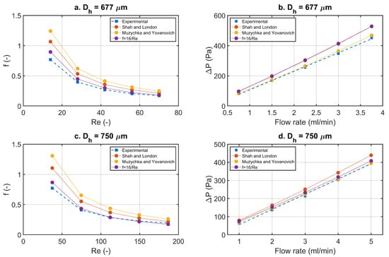
Figure 6.
Single phase pressure drop. Shah and London model from [42] and Muzychka and Yovanovich model from [43]. (a) Fanning friction of channel with 1.050 mm × 0.5 mm cross section. (b) pressure drop of channel with 1.050 mm × 0.5 mm cross section compared with predictive models. (c) Fanning friction of channel with 1.500 mm × 0.5 mm cross section. (d) pressure drop of channel with 1.500 mm × 0.5 mm cross section compared with predictive models.
Table 2.
Single phase pressure drop mean absolute error with prediction models.
4.2. Two Phase Experimental Results
Global pressure drop has been used to determine the boiling flow regime or the boiling quality in several contributions [2,5,29]. The advantage of this parameter is that it can be measured relatively easily with the necessary precision as compared to temperature measurement. However, pressure drop over the whole channel does not provide the local information. When two phase experiments were performed, high oscillation in the channel pressure was expected due to the volume expansion. Pressure drop oscillation during boiling is shown in Figure 7. The mass flux was fixed to 22.17 for all four subplots and heat flux was increased from left to right, (a) , (b) , (c) , and (d) . The black line in each subplot denotes the pressure drop of the same mass flux at room temperature. Pressure drop is a determining factor for the pump selection in the system design. Figure 7a illustrates the increase of the pressure drop by almost an order of the magnitude at the same liquid mass flux when boiling is happening in the microchannel, while drastic oscillations take place. This clearly highlights the need for prediction tools and methods for estimating pressure drop in order to bring two phase boiling into real world applications, especially in the design phase of new cooling devices. We observe that the oscillation period and amplitude is bigger at lower heat flow and is becoming more steady at higher heat flow like . We observed in the high speed frames that in , nucleation of single bubbles and enlargement (sometimes in reverse direction) happen more often. On the other hand, in relatively high heat fluxes, annular flow which was more stable occurred all along the channel and therefore the oscillation amplitude was relatively low.
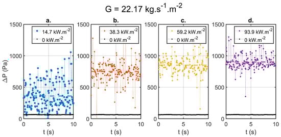
Figure 7.
Example of differential pressure drop in different wall heat flux with a constant mass flux of G = 22.17 in channel with 750 m. the black line indicates pressure drop in single phase in room temperature with the same mass flux. (a). . (b). . (c). . (d). .
Heat transfer coefficients were calculated as outlined above (Section 3) locally as well as averaged over channel length. Calculated values for h from experiments using mass flows between 22 and 95 and heat flux between 14.7 and 83.4 in the two micro channel sizes of hydraulic diameters of 677 and 750 respectively are shown in Figure 8. The heat transfer coefficients for the full channel length are shown in Figure 8a. In Figure 8b, only the channel length after reaching saturation temperature (in which phase change transfer occurred) are plotted. The linear regression mean heat transfer coefficient and heat flux is plotted in Figure 8 for (a) both single and two phase region and (b) just two phase region. The presented data in this figure cover the entire range of tested operating conditions. The slope of the linear regression corresponds to the mean surface and saturation temperature difference . The result shows that the mean surface and fluid temperature along the length of channel by considering both single and two phase regions can predict the heat transfer coefficient reasonably. This is due to the fact that most of experiments were conducted under subcooled boiling conditions. The heat flux is the superposition of both the liquid phase heat flux and the evaporation heat flux.
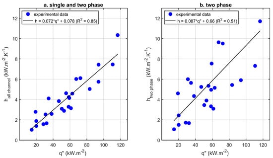
Figure 8.
Heat transfer coefficient versus heat flux. (a). Mean heat transfer coefficient for both single and two phase regions versus mean heat flux. (b). Mean heat transfer coefficient of two phase regions versus mean heat flux.
Figure 9 and Figure 10 illustrate the heat transfer coefficient versus vapor quality for the flow boiling experiments in a microchannel with hydraulic diameters m and m, respectively. They are displayed in four subfigures, each of which refers to a specific mass flow rate. They show mostly similar trend for different operating conditions. From the data in the figures, it is obvious that the higher vapor quality range was achieved at lower mass flow rate (refer to the difference in the x-axis-scaling). As the mass flux increases, the location where boiling starts moves further downstream, resulting in decreased the vapor quality range (or evaporation efficiency). These decrements correspond to the reduction in bubble frequency nucleation with increasing vapor quality and mostly bubbles tend to coalesce to form bigger bubbles. The heat transfer performances improve with the heat flux due to increasing the contribution of the nucleate boiling, as reported in many microchannel flow boiling literature [1,16,28].
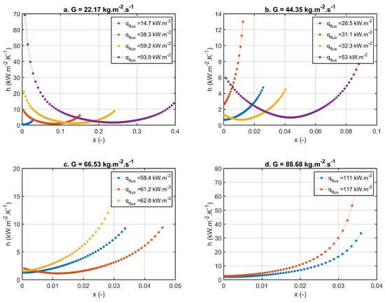
Figure 9.
Local boiling heat transfer coefficient vs. vapor quality for channel 1 with fixed mass flux in each subplot for channel 1.5 mm × 0.5 mm ( = 750 m). (a) G = 22.17 (b) G = 44.35 (c) G = 66.53 (d). G = 88.68 .
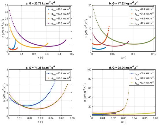
Figure 10.
Local boiling heat transfer coefficient vs. vapor quality for channel 2 with fixed mass flux in each subplot for channel 1.05 mm × 0.5 mm ( = 677 m). (a) G = 23.76 (b) G = 47.52 (c) G = 71.28 (d). G = 95.04 .
At relatively low mass flow rates and accordingly high heat flux rates (Figure 9a,b and Figure 10a–c), the highest heat transfer coefficient is observed at the start point of boiling for high heat flux rate due to the relatively high heat transfer performance. Thereafter h decreases at very low value of vapor quality. In relatively higher vapor quality range, the heat transfer coefficient rapidly increases with the vapor quality. The higher the value of the heat flux, the larger the heat transfer coefficient that is obtained. As reported in the literature, the minimum heat transfer coefficient happened at intermittent-annular flow pattern transition with a lot of suspended bubbles [44]. The corresponding vapor quality to the minimum heat transfer coefficient is called . For vapor quality higher than , a plateau trend exhibit for the heat transfer coefficient, while the nucleate boiling decrease and the convective boiling is dominant in this region. At relatively higher vapor quality region, when the flow regime is annular, the heat transfer coefficient increases again with vapor quality and convective boiling becomes the dominant heat transfer mechanism in this region. The ascending trend of h with x is seen at relatively low mass and heat fluxes (Figure 9a,b). In the remaining cases, at the beginning, h increases weakly with the vapor quality, which stays very low. This increase becomes steep at higher vapor quality values in the transition to annular flow. The increasing trend of h with increasing x in the slug flow, elongated bubble flow, and annular flow is due to the thin liquid film evaporation. Since the liquid film dry-out did not occur in the experiments, the descending trend of h at higher vapor quality region is not observed in Figure 9 and Figure 10.
The pressure drop of flow boiling in microchannels, hydraulic diameter (a) 750 m and (b) 677 m, versus the outlet vapor quality for different mass flow rate is shown in Figure 11. As expected, the pressure drop grows with increased mass flow rate in most of the cases, because increasing mass flux results in increased frictional pressure drop. There is an exception for mass flux 66.53 and 88.68 . This abnormality can be considered as an experimental outlier. The pressure drop also increases with outlet vapor quality. The outlet vapor quality arises due to higher heat flux which induces higher acceleration pressure and also increases the frictional pressure drop.
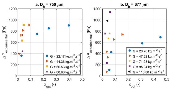
Figure 11.
Pressure drop vs. vapor. (a) channel cross Section 1.50 mm × 0.5 mm. (b) channel cross Section 1.050 mm × 0.5 mm.
Figure 12a–d show the data points predicted by four selected heat transfer correlations within ±30% error bands. All the selected correlations are able to predict the heat transfer coefficient of horizontal mini/microchannel flow boiling. The proposed correlations by Shah in 1977 [45], in 2017 [46], and Lee and Mudawar [47] were developed with a focus on subcooled boiling. Lee and Mudawar [47] conducted flow boiling experiments in horizontal, copper rectangular multimicrochannels with hydraulic diameter range 0.176–0.466 . The experiments were conducted at high mass flux 670,6730 and very low inlet temperature 0–30 . The correlation predicts 29.6% data in ±30% error bands with a mean average error of 69.3% (Figure 12b). The proposed correlations by Shah in 1977 [45] and 2017 [46] were developed based on a comprehensive database for different fluid such as water, refrigerants and chemicals through pipes, annuli, and channels. These correlations are presented in Figure 12a,c. Shah’s Correlation in 2017 [46] predicted 33.3% of the experimental data with a mean average error of 59.2%. The correlation of Shah 1977 [45] predicted only 22.2% of data with MAE of 46.9%. Mahmoud and Karayiannis [48] developed an empirical correlation based on 5152 data points in a heat flux range of 1.7–158 and mass flux range of 100–700 . They proposed this correlation for R134 flow boiling in vertical channels, but Sempertegui-Tapia and Ribatski [49] showed that it was also in good agreement with rectangular horizontal microchannels. As seen in Figure 12d, this correlation was able to predict 37% of the experiment data with a MAE of 39.7% and shows the closest prediction compared to others, as it is obvious the performance of the correlation is changed by decreasing the hydraulic diameter of the channel. As the hydraulic diameter decreases, the correlation predicted the data more accurately. The overall prediction possibility of acquired results versus available models is relatively poor. It is due to the fact that boiling mechanisms are heavily dependent on experimental conditions which need prediction methods, which are extremely well tailored to the experimental setup. On the other hand, a larger database should be generated to cover several fluids and different operating conditions for assessing the available correlations.
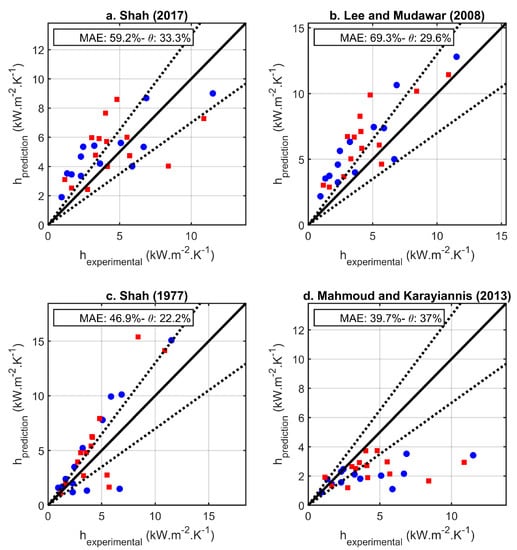
Figure 12.
Comparison of experimental results with existing heat transfer correlations. Red squares are acquired results from channel 1.5 mm × 0.5 mm and blue circles are acquired results from channel 1.05 mm × 0.5 mm. Dashed lines are depicting ±30% error band. (a) [46] (b) [47] (c) [45] (d) [48].
4.3. Local Electrical Sensing
To complement the pressure and temperature measurements, another technology, namely electric impedance measurements were introduced to characterize the flow regime, which has been identified as a very important characteristic for modeling evaporation. In these experiments, the impedance analyzer had an excitation AC frequency of 50 with 1 peak to peak voltage. The AC excitation frequency of the measurements was fixed to 50 kHz and data acquisition was performed in 13.7 kHz sampling rate. The sensors S1, S2, S3, and S4 were located along the channel as shown in Figure 13. A Matrix of impedance measurements with the application of 30 Watt total power using flow rates between 1 to 4 mL/min (22.17 to 88.68 ) four impedance sensor locations are shown in Figure 14. The probability density of each corresponding impedance measurement is depicted in Figure 15. The sensors are 1.7 mm wide and 2 mm long located on the 1.5 mm wide and 0.5 mm deep channel. In previous publications, the sensor fabrication, channel details method, and data acquisition with LCR-meter Hioki-IM3536 were reported [35,50,51]. In this work the test loop concept is similar but the LCR-meter is replaced with an impedance analyzer produced by Zurich Instruments (MFIA). The advantage of this newly developed system compared to our previous publication [35] is the time synchronization between the highspeed videos and impedance signals. The stainless steel channel is the counter electrode to the ITO electrode on the glass lid. The videos are used as the ground truth and the reference for signal analysis.
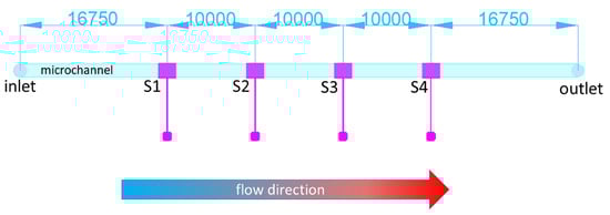
Figure 13.
Location of the sensors center with respect to the channel inlet center located along the channel.
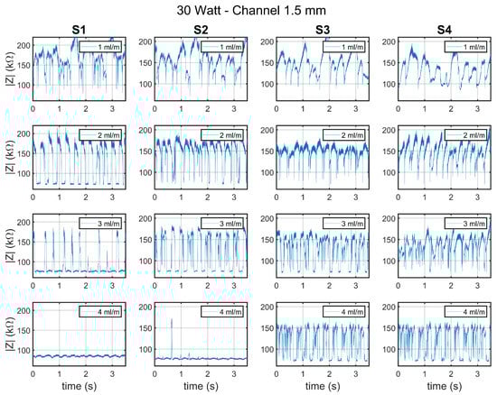
Figure 14.
Impedance measurements for 30 W experiments on channel 1.
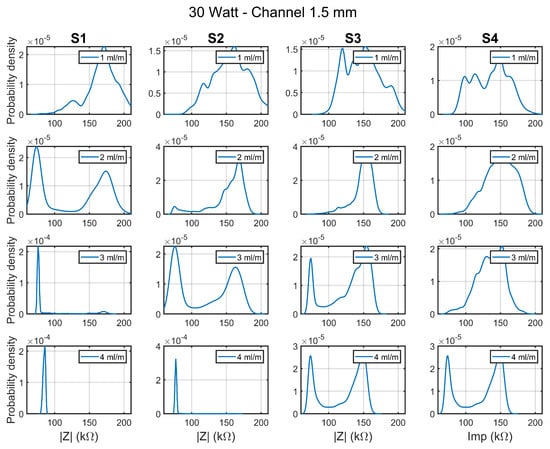
Figure 15.
Probability Density of impedance measurements for 30 W experiments on channel 1.
To discuss the application of impedance measurements in correlation with high speed videos, two measurements selected from Figure 14 and corresponding video are shown in Figure 16 for 1 (22.17 ) and 2 (44.35 ). In this figure, impedance amplitude measurements for 1.6 s long synced with highspeed photos recorded in 10 are shown which are corresponding to S1 location that its center is located 16.75 mm after the channel inlet center (see Figure 13 for sensor locations). In Figure 16a photos, we can see an example of annular flow in the channel with some anomalies in the thin layer around the vapor cylinder in the middle of the channel. The impedance level stays around ∼170 , but oscillations are observed due to instabilities in the flow. In annular flow, meanwhile, the flow maintains the thin layer around the vapor core in the channel; the changes in impedance level are attributed to thin layer size change. Moreover, temperature changes at the liquid in the change temperature can be another cause for such oscillations. However, in the probability density of the 30 Watt power and 1 mL/min (22.17 ) flow in S1 location as shown in Figure 15, a big peak is located at 170.62 and the smaller peak is located at 127.34 . The smaller peak in impedance is attributed to the thickenings in the liquid thin layer around the vapor cylinder (shown in Figure 16a at 26.1 and 27.4 ). The higher peak is attributed to annular flow with thin layer (such as Figure 16a pictures in 978 and 994 ). In Figure 16b, an example of typically occurring slug flow in the channel is illustrated. The video shows slugs nucleating around the sensor location and filling the channel very quickly. This slugs generate similar vapor cylinders to the annular flow; therefore, the impedance level when a slug is passing is similar to annular flow for the same sensor. The PDF curve for this impedance measurement has two peaks which are located in 73.9521 and 173.04 . These peaks are attributed to slug impedance and liquid impedance that are periodically passing under the electrode area. In the videos, it was observed that some slugs might have small interruptions. For example, the slug small discontinuity with liquid and followed by another slug is showed in 416.6 ms in Figure 16b. The corresponding drop in impedance amplitude to the same figure can be seen in the impedance signal as well. Another important observation is if slugs nucleate at some point after the senor/recording area, but the elongation is in reverse flow direction and therefore the sensor detects a slug. For example, in Figure 16b, at the photo with 275 ms timestamp the bubble nucleation point was not caught on the video since it was downstream of the sensor(and recording area) towards outlet. However, the slug elongated against the flow direction until it completely covered the sensor area. This highlights a limit of the impedance sensing method, which is the inability to detect the direction of vapor flow. The same kind of output for the slugs that were created before, in the sensor location, or after the sensor location was observed.
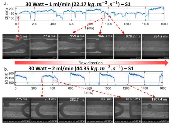
Figure 16.
Example of impedance measurements and high speed videos. (a). An example of annular flow impedance measurement and high-speed pictures. (b). An example of slug flow with high speed videos.
In Figure 17, an example of flow evolution along the channel with one power and flow rate set is illustrated. This example shows that in first (S1) and second (S2) sensor locations, slug flow is observed. The flow evolves to annular in S3 and S4 locations by absorbing more heat from the channel walls. Comparison between locations S1 and S2 make clear that slugs occupy the channel for longer periods of time at location S2 than at S1. This can be observed by probability density curves of these two impedance signals and are validated by highspeed videos. It is more likely to have a high impedance that lies in the range of 150 to 200 in S2 location as shown in Figure 17 that correlates with vapor core with thin layer around it. The physical reason behind this behavior is the development of bubbles and enlargement after liquid being exposed to the hot surface of the channel and absorbing heat. In the experiments, bubbly flow was observed very rarely due to the very quick transition from passing bubble to slugs happening when nucleation started in the channel.
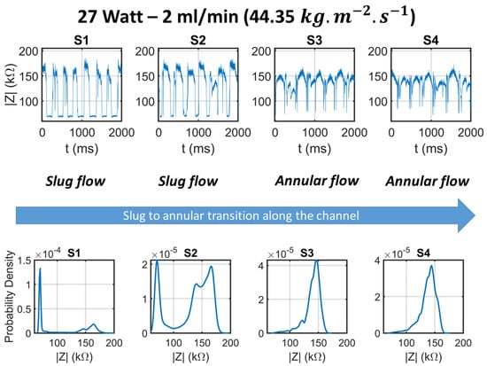
Figure 17.
Change of the signal and flow regime along the channel in four sensor locations.
Slug Flow Analysis Using Impedance Sensors
Figure 18 shows the synchronized photos of a slug passing under the electrode area in parallel with the impedance amplitude measurement. In this figure, it is shown that a bubble nucleates under the sensing area and slightly moves toward the inlet. Then by absorbing more heat from the channel, it starts expanding and turns into a long slug that covers the sensor area for almost 171 . The figure highlights the match between the detected signal of the beginning (green line at 1226 ms) and the end (red line with 1397 ms) of the slug phase. This video and impedance signal data points signal validation assures the usage of signal processing to determine important values based on signal processing such as slug period (), liquid period(), and slug frequency . Since the signal acquired in slug flow looks like a bilevel signal, we can analyze the slugs beginning and end time in each sensor location. It is important to know that each slug has a much larger size than the sensor area size and the rising and the falling signal is very steep. Therefore, it is plausible to consider the results of the impedance post processing as local or cross sectional information in the sensor center. The probability density of a slug flow causes two major peaks as explained above in probability density curve; therefore, by dividing the probability density data into two subhistograms optimized by minimum variance in each subhistogram, the state levels can be derived. The post processing method details using statelevels function in MATLAB for finding slug and liquid impedance levels are explained previously in [36]. The statelevels function in our case was set with a 10 percent tolerance for detecting fall/rise timestamps of each passing slug under the sensor. Thestatelevel is chosen high enough to include the slugs that have thicker liquid around them and consequently, they show a lower impedance amplitude. If the boundary levels are not wide enough (for example tolerance 1 or 2 percent), some slugs will not be counted. A full signal for ∼5 s is shown in Figure 19c that shows how the impedance level of vapor might be at lower level for some slugs comparing to others. To evaluate quantitatively, an image processing algorithm is needed that compares length of the slugs with the signals acquired. This is not possible at the moment due to high technical overhead and extreme flow instabilities. Increasing the tolerance level to a higher number like 15 percent will not make a difference in the slug frequency.
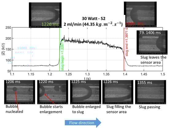
Figure 18.
Example of synchronized recorded photos and impedance amplitude measurement. The green and red vertical lines are derived from signal post processing.
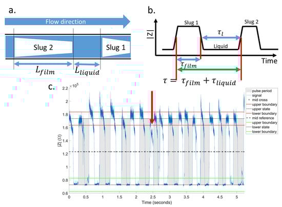
Figure 19.
(a) Representation of slugs in updated 3-zone-model passing in microchannel boiling [8]. (b) Impedance measurements signal using implemented sensors [36]. (c) Slug flow impedance signal for 5 s. The red arrow shows an example of a slug that has lower impedance level comparing to the other slugs impedance amplitude.
In Figure 20, the impedance amplitude measurements of three different experiments are shown. Pulse width in subfigures d to e denote and pulse period is representative of for each pulse. These values are calculated using functions in MATLAB called “pulseperiod” and “pulsewidth” with tolerance level set to 10 percent. For the signals shown in Figure 20a–c, the mean slug frequencies are respectively 3.85 Hz, 4.41 Hz, and 3.89 Hz and the mean duty cycles () are 0.52, 0.63, and 0.31. Duty cycle is a determining value in local heat transfer, since during thin film evaporation the heat transfer can be one order of magnitude higher than in liquid single phase.
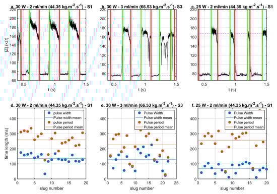
Figure 20.
Example of electrical sensing for slug flow. The green vertical lines show the beginning and of the slug and red vertical lines denote end of passing slug. (a) impedance amplitude with total power 30 and flow rate 2 mL/min (44.35 ) ( in S1 location. (b) impedance amplitude with total power 30 and flow rate 3 mL/min (66.53 ) in S3 location. (c) impedance amplitude with total power 25 and flow rate 2 mL/min (44.35 ) in S1 location. (d) pulse width and pulse period with impedance amplitude with total power 30 and flow rate 2 mL/min (44.35 ) in S1 location. (e) pulse width and pulse period with impedance amplitude with total power 30 and flow rate 3 ml/m in S3 location. (f). pulse width and pulse period with impedance amplitude with total power 30 and flow rate 2 mL/min (44.35 ) in S1 location.
A well known mechanistic model for predicting slug flow heat transfer coefficient is 3 zone model created by Thome et al. [52] in 2004 and further developed by Magnini et al. [8] and used by Falsetti et al. [33]. As Magnini et al. [8] reported, the model needs liquid slug length and bubble frequency for the prediction of the heat transfer coefficient as represented in Figure 19. The updated 3-zone model predicts slug flow heat transfer based on Equation (16) in which denotes the liquid parts passing heat transfer coefficient and represents heat transfer coefficient of the film. However, in heat transfer studies such as the one reported by Magnini et al. [8] both values, for bubble frequency and residence time, have been unknown due to the lack of a measurement method and were estimated based on other values. It is evident considering Equation (16), that knowing residence times of slug and liquid respectively play a pivotal role for taking advantage of Thome model.
Here, (see Figure 19). Magnini et al. [8] and Falsetti et al. [33] estimated slug frequency by minimizing deviation between experimental and predicted heat transfer coefficient. The and values are experimentally unknown when the prediction models were developed. As we show with three experimental examples in Figure 20, the beginning and end of each slug can be detected taking advantage of the acquired bilevel impedance signal. Therefore, pulse period () and pulse width () are derived from the impedance level detection and are shown in the plots below the impedance measurements. Therefore, film evaporation heat transfer can be predicted using Equation (17) [33]. is liquid film thickness at the end of bubble and is initial liquid film thickness, that are calculated by corresponding equations as shown in detail in Appendix B.
On the other hand, the heat transfer in the liquid passing period is considered as single phase heat transfer which can be predicted by several predictive models such as model suggested by Shah [42] shown in Equation (18). We do keep in mind that the Reynolds number in slugs is not necessarily reflecting the flow regime as in a developed single phase flow as was the condition when shah formulated the equation.
Using the above-mentioned correlations, and using results from the impedance measurements in the updated 3-zone model (Figure 20a) for the experiment at 30 and 2 mL/min (44.35 ) in position S1, we obtain and . Over a time period of 5.2 s, the local average heat transfer coefficient is estimated to be 33.03 .
In this section, we have shown three main features and advantages of having integrated electrical sensing over microchannel boiling test setups. First, we can recognize flow regime based on probability density curve of impedance amplitude in each location [35]. Second, it is possible to see anomalies and disturbances in annular flow thin layer as shown in Figure 16a and slug disconnection as illustrated by Figure 16b. These pieces of evidence were illustrated by synchronized images with the signals. Third, we have shown that local sensing can function as input to improve the usage of heat transfer predictive models. Impedance sensors response can be considered instant in comparison to temperature sensing and has the advantage of scaling possibilities in comparison to visualization. In our case, we showed how our sensors can shed a light on slug frequency and residence time and provide local information. These values were used in a showcase as input into the 3 zone model by Thome [33,52].
5. Summary
In this work, we presented an experimental analysis of DI-water evaporation in a single microchannel with hydraulic diameters of 750 and 677 , respectively. The test setup enabled local electrical sensing and simultaneous video recording. Full thermodynamic data reduction analysis of the results obtained in the test setup has been performed. Following points are concluded from the results and observations. The local flow boiling heat transfer coefficient was experimentally calculated and the influence of the experimental conditions such as the mass flow rate, heat flux and hydraulic diameter of channel were evaluated. The heat transfer coefficient evolution with the vapor quality was discussed for various combinations of heat flux and mass flow rate. The total pressure drop along side the channel for single phase and boiling part was measured. The effect of the mass flow rate and heat flux value on that was also evaluated.
- It was found that the flow regime in the channels varied considerably between the selected experimental conditions.
- Two different regimes were identified for the value of the heat transfer coefficient with respect to the vapor quality within the investigated mass and heat flux conditions: At the onset of evaporation (0 < x < 0.05), the heat transfer coefficient increases with the vapour quality. At intermediate vapor quality ranges (0.05 < x < 0.5), the heat transfer coefficient shows a “U” shape profile. Since the dry-out did not occur in any of the experiments, the heat transfer coefficient did not decrease to a value typical for gas systems.
- For the heat transfer coefficient, a similar comparison was done using four correlations. It was found that most correlations predicted the correct values for some points but failed in other regimes. The correlation published by Mahmoud and Karayianis [48] showed the best predictive performance over the whole range of experiments. There are relatively big mean absolute error values observed between experimental results and prediction of the selected correlations. We conclude that this is due to the relative unstable and different flow conditions.
- It was affirmed that it is possible to find local information regarding the flow regime using impedance sensors as we presented previously in [35]. In most conditions, slug flow and annular flow regimes were observed in the channel. In the instances when bubbly flow was found, it transformed into slug flow. The application of such sensing system was highlighted in mechanistic models based on flow regime such as the model presented by Falsetti et al. [33].
- The slug passing frequency and duty cycle are critical and usable information that was obtained and cross checked with the synchronized videos. Thus for the case when slug flow is the dominant regime in the channel, the information gleaned form the impedance spectroscopy, namely residence time and bubble frequency at the sensor location is very useful.
- Since it has been found that the flow regime is of paramount importance regarding the heat transfer, the information gained from impedance spectroscopy is a useful tool to use the correct correlations for a given set of experimental conditions.
At this stage, it is challenging to export meaningful feed in information from impedance measurements for annular flow, especially regarding thin layer thickness. The major reason is having high temperature oscillations and differences in each test, which results in change of absolute value in impedance amplitude measurements. Moreover, we intend to use sensing elements as a direct feed-in for active nucleation in the channel, for understanding the stabilization methods in microchannel boiling. The connection between local void fraction and impedance sensing has been analyzed by several researchers based on Maxwell-Garnett impedance approximations such as Rosa et al. [53]. By determining flow temperature, the mixture impedance has the potential to be further related to local void fraction. This can be helpful to develop more accurate heat transfer models for each particular flow pattern, especially annular flow.
Another interesting application for this sensing would be refining the heat transfer models by such sensors. The authors have outlook of having time transient heat transfer of the test setup and widening the application for the presented impedimetric sensing method as feed in for heat transfer model. Further usage of different refrigerants in addition to DI-water as working fluid will make experimental data sets bigger and consequently better comparison with predictive models will be acquired. For example, Falsetti et al. suggests a flow pattern based mechanistic model based on convective boiling in slug flow and annular flow [33]. In this model, two main flow regimes are considered and the transition between slug to annular flow transition between them is solved by using a smoothing function. Having such sensing system, it is possible to understand the flow regime and take advantage of prediction models functioning based on flow regimes along the channel. The possibility of using local electrical sensors as feed in for heat transfer models can extend the possibility of studying heat transfer in microchannels, since larger piles of data can be analyzed without personal supervision and visual inspection.
Author Contributions
Conceptualization, M.K., R.D., and P.W.; Data curation, M.T. and S.S.; Funding acquisition, R.D. and P.W.; Investigation, M.T., S.S., and M.K.; Methodology, M.T. and S.S.; Project administration, M.K., R.D., and P.W.; Resources, R.D. and P.W.; Software, M.T.; Supervision, M.K., R.D., and P.W.; Validation, M.T. and S.S.; Visualization, M.T.; Writing—original draft, M.T. and S.S.; Writing—review and editing, M.T., S.S., M.K., and P.W. All authors have read and agreed to the published version of the manuscript.
Funding
Financial support by the German Research Foundation (DFG) through the Research Unit FOR 2383 ProMiSe is gratefully acknowledged. The article processing charge was funded by the Baden-Wuerttemberg Ministry of Science, Research and Art and the University of Freiburg in the funding program Open Access Publishing.
Acknowledgments
We appreciate the support given by IMTEK cleanroom staff for glass lid fabrication process. The kind help and support for housing machining from Franz Richard and Heinz Lambach is gratefully acknowledged. The authors would like to thank Liang Schengzi for 2D code implementation.
Conflicts of Interest
The authors declare no conflict of interest.
Nomenclature
| A | cross-section area | () |
| heat capacity | () | |
| hydraulic diameter | () | |
| f | friction factor | (-) |
| G | mass flux | () |
| h | heat transfer coefficient | () |
| latent heat of vaporization | () | |
| channel height | () | |
| I | electrical current | () |
| k | thermal conductivity | () |
| K | pressure loss coefficient | (-) |
| L | channel length | () |
| heat flux | () | |
| power | () | |
| t | time | () |
| T | temperature | () |
| V | electrical voltage | () |
| channel width | () | |
| x | vapor quality, | (-) |
| void fraction | (-) | |
| channel aspect ratio | (-) | |
| liquid film thickness | () | |
| dynamic viscosity | () | |
| density | () | |
| time period | () | |
| two phase multiplier | (-) | |
| Dimensionless numbers | ||
| Boiling number | ||
| Bond number | ||
| C | Chisholm parameter | |
| Martinelli parameter | ||
| Froude number, | ||
| Nusselt number | ||
| Peclet number, | ||
| Prandtl number, | ||
| Reynolds number, | ||
| Webber number, | ||
| Subscripts | ||
| acceleration | ||
| ambient | ||
| base | ||
| channel | ||
| expansion | ||
| effective | ||
| fluid | ||
| footprint | ||
| v | vapor | |
| inlet | ||
| l | liquid | |
| local | ||
| heat loss | ||
| outlet | ||
| saturation | ||
| single phase | ||
| two phase | ||
| w | wall | |
| sudden contraction | ||
| sudden expansion | ||
| corner | ||
Appendix A. Single Phase Pressure Drop
In case of having a single phase flow along the channel without any boiling and bubble formation, the flow can be divided to developing flow and fully developed flow. is the length of single phase flow and and denotes length of fully developed flow. In the developing region where , both fluid acceleration and shear stress between wall and fluid contribute in pressure drop. In the fully developed region, where , the friction factor is only resulted from shear stress between the fluid and channel. Two correlations describe the pressure drop of the single phase flow in a rectangular microchannel. The first model is proposed by Shah and London [42]. The length of the developing fling flow is calculated using Equation (A1).
In Shah and London model, the friction factor for developing flow in single phase is shown in Equation (A2a,b).
and for fully developed flow friction factor is shown in Equation (A3) based on aspect ratio .
In another correlation reported by Muzychka and Yovanovich [43,54], the characteristic length for the developed flow is calculated by Equation (A4).
where is
and is calculated by channel aspect ratio
The friction factor for developing flow is shown by Equation (A7) as follows
and the friction factor in developed flow is calculated as following
Appendix B. Boiling Heat Transfer Coefficient Correlations
The equations corresponding to the heat transfer coefficient correlations used in Figure 12 are shown as follows.
The correlation provided by Lim et al. at 2014 is shown by Equation (A9a,b) [55].
The correlation that was provided by Shah is shown in Equation (A10a) in which the two phase heat transfer is derived from single phase heat transfer coefficient as shown by Equation (A10b) [46].
Another correlation by Shah [45] which is modified considering subcooling is shown in Equation (A11a).
As Falsetti et al. presented [33], for using 3-zone model, film thickness () is considered as the minimum of the (film thickness for long traveling bubbles at a constant speed), (film thickness for accelerating bubble), (the thickness of the viscous boundary layer at the wall in the liquid slug between two bubbles) [33]. The value of in Equation (A14c) can be different for each single slug and in each specific point of the channel along z direction but having local impedance measurements it can be derived by Equation (A13). can be calculated based on total mass flux based on Equation (A13).
References
- Kandlikar, S.G. History, Advances, and Challenges in Liquid Flow and Flow Boiling Heat Transfer in Microchannels: A Critical Review. J. Heat Transf. 2012, 134. [Google Scholar] [CrossRef]
- Karayiannis, T.; Mahmoud, M. Flow boiling in microchannels: Fundamentals and applications. Appl. Therm. Eng. 2017, 115, 1372–1397. [Google Scholar] [CrossRef]
- Huang, H.; Thome, J.R. An experimental study on flow boiling pressure drop in multi-microchannel evaporators with different refrigerants. Exp. Therm. Fluid Sci. 2017, 80, 391–407. [Google Scholar] [CrossRef]
- Bigham, S.; Moghaddam, S. Physics of the Microchannel Flow Boiling Process and Comparison with the Existing Theories. J. Heat Transf. 2017, 139, 111503. [Google Scholar] [CrossRef]
- Harirchian, T.; Garimella, S.V. A comprehensive flow regime map for microchannel flow boiling with quantitative transition criteria. Int. J. Heat Mass Transf. 2010, 53, 2694–2702. [Google Scholar] [CrossRef]
- Al-Zaidi, A.H.; Mahmoud, M.M.; Karayiannis, T.G. Flow boiling of HFE-7100 in microchannels: Experimental study and comparison with correlations. Int. J. Heat Mass Transf. 2019, 140, 100–128. [Google Scholar] [CrossRef]
- Bigham, S.; Moghaddam, S. Microscale study of mechanisms of heat transfer during flow boiling in a microchannel. Int. J. Heat Mass Transf. 2015, 88, 111–121. [Google Scholar] [CrossRef]
- Magnini, M.; Thome, J. An updated three-zone heat transfer model for slug flow boiling in microchannels. Int. J. Multiph. Flow 2017, 91, 296–314. [Google Scholar] [CrossRef]
- Kandlikar, S.G. Scale effects on flow boiling heat transfer in microchannels: A fundamental perspective. Int. J. Therm. Sci. 2010, 49, 1073–1085. [Google Scholar] [CrossRef]
- Li, W.; Yang, F.; Alam, T.; Qu, X.; Peng, B.; Khan, J.; Li, C. Enhanced flow boiling in microchannels using auxiliary channels and multiple micronozzles (I): Characterizations of flow boiling heat transfer. Int. J. Heat Mass Transf. 2018, 116, 208–217. [Google Scholar] [CrossRef]
- Li, W.; Wang, Z.; Yang, F.; Alam, T.; Jiang, M.; Qu, X.; Kong, F.; Khan, A.S.; Liu, M.; Alwazzan, M.; et al. Supercapillary Architecture Activated Two-Phase Boundary Layer Structures for Highly Stable and Efficient Flow Boiling Heat Transfer. Adv. Mater. 2019, 32, 1905117. [Google Scholar] [CrossRef] [PubMed]
- Li, W.; Alam, T.; Yang, F.; Qu, X.; Peng, B.; Khan, J.; Li, C. Enhanced flow boiling in microchannels using auxiliary channels and multiple micronozzles II: Enhanced CHF and reduced pressure drop. Int. J. Heat Mass Transf. 2017, 115, 264–272. [Google Scholar] [CrossRef]
- Prajapati, Y.K.; Pathak, M.; Khan, M.K. Bubble dynamics and flow boiling characteristics in three different microchannel configurations. Int. J. Therm. Sci. 2017, 112, 371–382. [Google Scholar] [CrossRef]
- Ozdemir, M.R.; Mahmoud, M.M.; Karayiannis, T.G. Flow Boiling of Water in a Rectangular Metallic Microchannel. Heat Transf. Eng. 2020, 1–25. [Google Scholar] [CrossRef]
- Mahmoud, M.M.; Karayiannis, T.G. Flow Boiling in Mini to Microdiameter Channels. In Encyclopedia of Two-Phase Heat Transfer and Flow IV; World Scientific: Singapore, 2018; pp. 233–301. [Google Scholar] [CrossRef]
- Cheng, L.; Xia, G. Fundamental issues, mechanisms and models of flow boiling heat transfer in microscale channels. Int. J. Heat Mass Transf. 2017, 108, 97–127. [Google Scholar] [CrossRef]
- Cheng, L.; Ribatski, G.; Thome, J.R. Two-phase flow patterns and flow-pattern maps: Fundamentals and applications. Appl. Mech. Rev. 2008, 61, 050802. [Google Scholar] [CrossRef]
- Cheng, L. Flow Boiling Heat Transfer with Models in Microchannels. In Microchannel Phase Change Transport Phenomena; Elsevier: Amsterdam, The Netherlands, 2016; pp. 141–191. [Google Scholar] [CrossRef]
- Kim, S.M.; Mudawar, I. Review of databases and predictive methods for heat transfer in condensing and boiling mini/micro-channel flows. Int. J. Heat Mass Transf. 2014, 77, 627–652. [Google Scholar] [CrossRef]
- Anwar, Z.; Palm, B.; Khodabandeh, R. Flow boiling heat transfer, pressure drop and dryout characteristics of R1234yf: Experimental results and predictions. Exp. Therm. Fluid Sci. 2015, 66, 137–149. [Google Scholar] [CrossRef]
- Zhuan, R.; Wang, W. Boiling heat transfer characteristics in a microchannel array heat sink with low mass flow rate. Appl. Therm. Eng. 2013, 51, 65–74. [Google Scholar] [CrossRef]
- Kim, S.M.; Mudawar, I. Universal Approach to Predicting Saturated Flow Boiling Heat Transfer in Mini Micro-Channels–Part II. Two-Phase Heat Transfer Coefficient. Int. J. Heat Mass Transf. 2013, 64, 1239–1256. [Google Scholar] [CrossRef]
- Qu, W.; Mudawar, I. Flow boiling heat transfer in two-phase micro-channel heat sinks––I. Experimental investigation and assessment of correlation methods. Int. J. Heat Mass Transf. 2003, 46, 2755–2771. [Google Scholar] [CrossRef]
- Mortada, S.; Zoughaib, A.; Arzano-Daurelle, C.; Clodic, D. Boiling heat transfer and pressure drop of R-134a and R-1234yf in minichannels for low mass fluxes. Int. J. Refrig. 2012, 35, 962–973. [Google Scholar] [CrossRef]
- Szczukiewicz, S.; Magnini, M.; Thome, J. Proposed models, ongoing experiments, and latest numerical simulations of microchannel two-phase flow boiling. Int. J. Multiph. Flow 2014, 59, 84–101. [Google Scholar] [CrossRef]
- Mukherjee, A. Contribution of Microlayer Evaporation During Flow Boiling Inside Microchannels. In Proceedings of the ASME 2008 6th International Conference on Nanochannels, Microchannels, and Minichannels (ASMEDC), Darmstadt, Germany, 23–25 June 2008. [Google Scholar] [CrossRef]
- Yin, L.; Jia, L.; Guan, P. Bubble confinement and deformation during flow boiling in microchannel. Int. Commun. Heat Mass Transf. 2016, 70, 47–52. [Google Scholar] [CrossRef]
- Thome, J.R.; Consolini, L. Mechanisms of Boiling in Micro-Channels: Critical Assessment. Heat Transf. Eng. 2010, 31, 288–297. [Google Scholar] [CrossRef]
- Huh, C.; Kim, M.H. Pressure Drop, Boiling Heat Transfer and Flow Patterns during Flow Boiling in a Single Microchannel. Heat Transf. Eng. 2007, 28, 730–737. [Google Scholar] [CrossRef]
- Cheng, L. Flow Patterns and Bubble Growth in Microchannels. In Microchannel Phase Change Transport Phenomena; Elsevier: Amsterdam, The Netherlands, 2016; pp. 91–140. [Google Scholar] [CrossRef]
- Jagirdar, M.; Lee, P.S. Study of transient heat transfer and synchronized flow visualizations during sub-cooled flow boiling in a small aspect ratio microchannel. Int. J. Multiph. Flow 2016, 83, 254–266. [Google Scholar] [CrossRef]
- Piasecka, M.; Strak, K.; Maciejewska, B. Calculations of Flow Boiling Heat Transfer in a Minichannel Based on Liquid Crystal and Infrared Thermography Data. Heat Transf. Eng. 2017, 38, 332–346. [Google Scholar] [CrossRef]
- Falsetti, C.; Magnini, M.; Thome, J. A new flow pattern-based boiling heat transfer model for micro-pin fin evaporators. Int. J. Heat Mass Transf. 2018, 122, 967–982. [Google Scholar] [CrossRef]
- Kandlikar, S.G. High Flux Heat Removal with Microchannels—A Roadmap of Challenges and Opportunities. Heat Transf. Eng. 2005, 26, 5–14. [Google Scholar] [CrossRef]
- Talebi, M.; Sadir, S.; Cobry, K.; Stroh, A.; Dittmeyer, R.; Woias, P. Investigation of water microchannel boiling flow regimes using electrical sensing elements along a single microchannel. Meas. Sci. Technol. 2019, 30, 125301. [Google Scholar] [CrossRef]
- Talebi, M.; Baeumker, E.; Cobry, K.; Sadir, S.; Stroh, A.; Woias, P. Investigation of Slug Flow in Microchannel Boiling by Impedimetric Sensing. In Proceedings of the 2019 IEEE SENSORS, Montreal, QC, Canada, 27–30 October 2019; pp. 1–4. [Google Scholar] [CrossRef]
- Talebi, M.; Cobry, K.; Sadir, S.; Dittmeyer, R.; Woias, P. Flow Regime Detection of Boiling Flow in Microchannels Using Electrical Sensing Elements Validated by Videography. In Proceedings of the ASME 2018 16th International Conference on Nanochannels, Microchannels, and Minichannels. American Society of Mechanical Engineers, Dubrovnik, Croatia, 10–13 June 2018; p. V001T02A016. [Google Scholar]
- Pico Technology USB TC-08-Channel Thermocouple Data Logger Data Sheet, 9th ed.; Pico Technology Ltd.: St Neots, UK, 2019.
- Product Information mzr-7205 · High Performance Pump Series; HNP Mikrosysteme GmbH: Schwerin, Germany, 2019.
- Kenning, D.B.R.; Lewis, J.S.; Karayiannis, T.G. Pressure drop and heat transfer characteristics for single-phase developing flow of water in rectangular microchannels. J. Phys. Conf. Ser. 2012, 395, 012085. [Google Scholar] [CrossRef]
- Zohuri, B. Compact Heat Exchangers; Springer International Publishing: Berlin/Heidelberg, Germany, 2017. [Google Scholar] [CrossRef]
- Shah, R.; London, A. Laminar Flow Forced Convection in Ducts; Elsevier: Amsterdam, The Netherlands, 1978. [Google Scholar] [CrossRef]
- Muzychka, Y.S.; Yovanovich, M.M. Pressure Drop in Laminar Developing Flow in Noncircular Ducts: A Scaling and Modeling Approach. J. Fluids Eng. 2009, 131. [Google Scholar] [CrossRef]
- Da Silva Lima, R.J.; Quibén, J.M.; Thome, J.R. Flow boiling in horizontal smooth tubes: New heat transfer results for R-134a at three saturation temperatures. Appl. Therm. Eng. 2009, 29, 1289–1298. [Google Scholar] [CrossRef]
- Shah, M. A General Correlation for Heat Transfer during Subcooled Boiling in Pipes and Annuli. In Proceedings of the ASHRAE Semiannual Meeting, Chicago, IL, USA, 13–17 February 1977; pp. 202–217. [Google Scholar]
- Shah, M.M. New correlation for heat transfer during subcooled boiling in plain channels and annuli. Int. J. Therm. Sci. 2017, 112, 358–370. [Google Scholar] [CrossRef]
- Lee, J.; Mudawar, I. Fluid flow and heat transfer characteristics of low temperature two-phase micro-channel heat sinks – Part 2. Subcooled boiling pressure drop and heat transfer. Int. J. Heat Mass Transf. 2008, 51, 4327–4341. [Google Scholar] [CrossRef]
- Mahmoud, M.M.; Karayiannis, T.G. Heat transfer correlation for flow boiling in small to micro tubes. Int. J. Heat Mass Transf. 2013, 66, 553–574. [Google Scholar] [CrossRef]
- Sempértegui-Tapia, D.F.; Ribatski, G. Flow boiling heat transfer of R134a and low GWP refrigerants in a horizontal micro-scale channel. Int. J. Heat Mass Transf. 2017, 108, 2417–2432. [Google Scholar] [CrossRef]
- Talebi, M.; Woias, P.; Cobry, K. Analysis of impedance data from bubble flow in a glass/SU8 microfluidic device with on-channel sensors. Sens. Actuators Phys. 2018, 279, 543–552. [Google Scholar] [CrossRef]
- Talebi, M.; Cobry, K.; Zhou, Z.; Sadir, S.; Dittmeyer, R.; Woias, P. Investigation of boiling phenomena in microchannels using impedance spectroscopy technique correlated with videography. In Proceedings of the MikroSystemTechnik (Congress 2017), Munich, Germany, 23–25 October 2017; pp. 1–4. [Google Scholar]
- Thome, J.; Dupont, V.; Jacobi, A. Heat transfer model for evaporation in microchannels. Part I: Presentation of the model. Int. J. Heat Mass Transf. 2004, 47, 3375–3385. [Google Scholar] [CrossRef]
- Rosa, E.S.; Flora, B.F.; Souza, M.A.S.F. Design and performance prediction of an impedance void meter applied to the petroleum industry. Meas. Sci. Technol. 2012, 23, 055304. [Google Scholar] [CrossRef]
- Muzychka, Y.S.; Yovanovich, M.M. Laminar Forced Convection Heat Transfer in the Combined Entry Region of Non-Circular Ducts. J. Heat Transf. 2004, 126, 54–61. [Google Scholar] [CrossRef]
- Lim, T.W.; You, S.S.; Choi, J.H.; Kim, H.S. Experimental Investigation of Heat Transfer in Two-phase Flow Boiling. Exp. Heat Transf. 2014, 28, 23–36. [Google Scholar] [CrossRef]


Publisher’s Note: MDPI stays neutral with regard to jurisdictional claims in published maps and institutional affiliations. |
© 2020 by the authors. Licensee MDPI, Basel, Switzerland. This article is an open access article distributed under the terms and conditions of the Creative Commons Attribution (CC BY) license (http://creativecommons.org/licenses/by/4.0/).