Spatio-Temporal Kriging Based Economic Dispatch Problem Including Wind Uncertainty

Abstract

The integration of renewable generation adds complexity to the operation of the power system due to its unpredictable characteristics. Therefore, the development of methods to accurately model the uncertainty is necessary. In this paper, the spatio-temporal kriging and analog approaches are used to forecast wind power generation and used as the input to solve an economic dispatch problem, considering the uncertainties of wind generation. Spatio-temporal kriging captures the spatial and temporal information available in the database to improve wind forecasts. We evaluate the performance of using the spatio-temporal kriging, and comparisons are carried out versus other approaches in the framework of the economic power dispatch problem, for which simulations are developed on the modified IEEE 3-bus and IEEE 24-bus test systems. The results demonstrate that the use of kriging based spatio-temporal models in the context of economic power dispatch can provide an opportunity for lower operating costs in the presence of uncertainty when compared to other approaches.

1. Introduction

Renewable generation has received interest over the last few decades due to its environmentally sustainable and cost-effective operation relative to traditional energy sources. The integration of this intermittent energy into the power grid presents a range of challenges in the operation and management of these systems because energy cannot be dispatched in the conventional sense [1,2,3,4]. The scheduling of wind generation into the grid is a complex decision-making problem due to the variability implicit in wind resource availability. Addressing the uncertainty of renewable generations is crucial to increase economic benefits and enforce the criteria of reliability for decision-making [1].

Wind is influenced by temperature, humidity, direction, and certain factors, which can lead to unpredictable behavior. Besides, it is non-stationary and typically has strong diurnal and seasonal trends. It is also temporally and spatially auto-correlated and demonstrates heteroscedasticity. It is, therefore, a physical phenomenon in which modeling is challenging due to its characteristics [2]. Consequently, there is a requirement to develop more reliable, scalable, and realistic alternatives to modeling renewable generation uncertainties in order to accommodate a higher penetration of renewable energy sources into the grid [1].

1.1. Current Research

In the literature, there is a broad range of methods for forecasting wind speed and converting these values into wind power forecasts using power curves [1,2,5]. A widely used approach to represent renewable energy uncertainties is the creation of a set of time series called scenarios for forecasting the future [2]. The scenario approach has played an essential role in several stochastic and robust optimization problems, such as Unit Commitment (UC) [6,7], Economic Dispatch (ED) [8,9,10] , Energy trading policy [6], and Storage capacity sizing [11].

Although commonly used, generating scenarios that are capable of accurately informing system operators of power generation uncertainties remains a challenging problem [1]. The complexity of modeling unknown stochastic processes related to renewable energy is one of the most critical challenges in the generation of scenarios. Researchers have performed extensive work on the use of probabilistic and statistical models. In [12], Gaussian copula functions were used to generate statistical scenarios that took into consideration the complete temporal dependency structure of wind speed. Salehi Borujeni et al. [13] examined tail dependency when choosing the copula function for wind speed modeling. Meibom et al. [4] used the Auto-Regressive Moving Average (ARMA) time series and Monte Carlo simulation to generate a set of wind speed and load forecast error scenarios. A comprehensive modeling approach for multi-site wind power generation scenarios was presented in [2]. The model uses time series and principal components techniques, along with data preprocessing techniques to capture wind characteristics from multiple sites.

Nevertheless, most of the methods listed above require a significant amount of site-specific expertise for renewable resource modeling. The intermittent and time-varying characteristics of renewables and the complex dynamics of spatio-temporal interactions make it difficult to apply most of these approaches and tricky to implement them in practice [1,14]. Consequently, the scenarios generated may not adequately reflect the uncertainty of actual historical observations of renewable resources. Notwithstanding their computational benefits, the limited capacity of the mentioned models in capturing intricate patterns of correlations in real-world processes has encouraged the science community in the last decade to develop groups of models that capture spatial-temporal interactions.

In spatio-temporal modeling, both spatial and temporal variations of wind speed are taken into account in one model, and the prediction is made accordingly.

Table 1. Spatial-temporal methods applied to operational planning of power systems. STV, spatial-temporal variable; PFCST, point forecasting; Scen, scenario; TF, time frame; PLNG, power planning studies.

Ref.	Subject			STV			PFCST	Scen.	TF	Model
	FCST	PLNG	UC/ED	Wind	Solar	Demand
[15,16]			✓	✓			✓		short	Trigonometric direction diurnal model
[17]		✓			✓				short	Compressive spatio-temporal forecasting
[18]		✓		✓			✓		short	Spatio-temporal Markov chain
[19]		✓		✓			✓		short	Copula function
[20]	✓			✓			✓		short/long	Spatio-temporal covariance model
[21]		✓			✓		✓		short	QR-Lasso spatial-temporal
[22]	✓			✓			✓		short	Predictive deep convolutional neural network
[23]	✓			✓			✓		short	Spatio-temporal kriging
[24]	✓			✓			✓		short	Low-cost spatio-temporal adaptive filter
[25]	✓			✓			✓		short	Kernel methods
[26]	✓			✓			✓		short	Graph based convolution network
[27]		✓			✓		✓		short	Spatio-temporal model using clusters of meteorological conditions
[28,29]	✓			✓	✓		✓		short	Spatio-temporal kriging
[30]	✓			✓			✓		short	Universal kriging and a Bayesian dynamic model
[31]			✓	✓			✓		short	Finite state Markov chain model
[32]		✓		✓			✓		short	Bayesian spatio-temporal model
[33]	✓			✓			✓		short	Multi-channel ARMA model
[2]		✓		✓				✓	short	Principal component analysis-time series
[34]			✓	✓			✓		short	Dynamic uncertainty sets
[35]	✓				✓		✓		short	Vector autoregressive (VAR) framework
[36]			✓	✓				✓	short	Kriging model and importance sampling method
[37]	✓					✓	✓		short	Compressive sensing and structured-sparse recovery algorithms
[38]			✓	✓			✓		short	A modified regime-switching space-time diurnal (RSTD) model
Proposed			✓	✓				✓	short	Spatio-temporal kriging and analog models

highlights a summary of the works found in the literature on the use of spatio-temporal models in power systems, in particular for forecasting (FCST), power planning studies (PLNG), and unit commitment or economic dispatch. Notice that there is no single method to model the spatio-temporal relationship of the variable to be forecasted. Furthermore, Table 1 specifies the spatial-temporal variables (STV), whether a point forecasting is made (PFCST) or scenarios (Scen) are generated, the time frame (TF), and finally, the model used. The proposed model is included in Table 1 to observe the differences with respect to the cited literature. The checkmarks indicate the subject, the spatio-temporal variables, and the use of the forecasts generated by the methods listed.

In [17], for three separate weather variables, namely irradiance, ambient temperature, and wind speed, the forecasting was performed using a compressive spatio-temporal forecasting model. Then, the output of the PV power plant was estimated by applying a power conversion model. A spatio-temporal Markov chain model for wind power forecasting was proposed in [18]. It extends the traditional discrete-time Markov chain and incorporates off-site reference information to improve the forecast performance of regional wind farms. In [19], the spatial-temporal correlation between member wind farms and aggregate wind power was modeled on a joint distribution model based on copula theory. Inverse sampling was applied to the joint distribution conditional (CDF) to generate aggregated probabilistic forecasts. In [20], the authors proposed a probabilistic framework for predicting wind speed from measured spatial-temporal data. The frame was based on the decomposition of spatial-temporal covariance and simulation using this decomposition. This framework allows temporal extrapolation and spatial interpolation. In [21], the authors proposed a probabilistic spatial-temporal model. The model is based on the quantile regression adapted to integrate the Lasso (least absolute shrinkage and selection operator) variable selection process. This makes it particularly suitable for situations in which data from a high number of PV installations are available since it is capable of dealing directly with the resulting high dimensionality and over-fitting issues that characterize the use of such large amounts of data. A deep convolution neural network topology for wind speed forecasting with spatio-temporal correlation (PDCNN) was presented in [22]. The model is a unified framework, integrating convolutional neural networks (CNNs) and a multi-layer perceptron (MLP). PDCNN generates the forecasted wind speed by using the spatial-temporal correlations learned. In [23], the authors proposed a covariance modeling approach that considers spatial-temporal anisotropy in the spatial-temporal kriging model. Spatial and temporal covariance functions are individually designed to generate synthetic wind power profiles to simulate the effects of fluctuations in power. The formulation of the Wiener cyclo-stationary filter was designed to predict wind based on its past values and the spatial-temporal correlation between the data measured in [24]. An iterative, stochastic gradient predictor that uses a multichannel least mean squares (LMS) algorithm has also been suggested. The Wiener cyclo-stationary filter and the LMS provide speed and direction predictions. Two non-linear methods for the production of short-term spatial-temporal wind speed forecasts were presented in [25]. A kernel least mean squares algorithm and a kernel least squares recursive algorithm were introduced and used to generate wind speed forecasts at different locations. In [26], a graph based convolution network was proposed for spatial-temporal wind speed forecasting. The proposed architecture was further improved by using the rough set theory to capture deep wind data interval features by incorporating upper and lower bound parameter approximations in the model. In [27], the authors proposed a spatial-temporal model that produces PV power forecasts for a power plant using measurements from other nearby plants. The method makes it possible to take into account local weather conditions in the spatial-temporal model. The model also incorporates the least absolute shrinkage and selection operator to improve the selection of variables.

Spatio-temporal correlations of irradiance data were analyzed for forecasting irradiance in [28,29]. Spatial and spatio-temporal methods were used for model irradiation at an arbitrary point based on a given time series irradiation at specific locations. In [30], the authors used an empiric variogram to analyze the spatial correlation of different locations on a wind farm. They used universal kriging and a Bayesian dynamic model for hierarchical wind farm modeling. Besides, the Gibbs sampling approach was used to analyze the model and to develop wind speed predictions. Lenzi et al. [32] proposed two Bayesian spatio-temporal models to obtain full probabilistic wind power forecasts. The models were based on a stochastic partial differential equation (SPDE) approach to spatio-temporal modeling, which enables rapid inference through integrated nested Laplace approximations (INLA), as well as dimensional reduction. Filik [33] proposed a multi-channel autoregressive moving average model (MARMA) for short-term wind speed forecasting using neighboring wind speed measurements around the target location. A comprehensive modeling methodology for multi-site wind power generation scenarios for forecasting power generation was presented in [2]. The model uses time series and principal component techniques along with pre-processing data techniques to directly capture the main wind characteristics from multiple locations, such as distinct diurnal and seasonal trends, non-Gaussianity, and spatial and temporal correlations.

The works mentioned above have only been used to predict or study the production of renewable energy. The implementation of the approaches and methods used for the operational planning of electrical systems has not been published.

The papers listed below were identified in the literature by the use of spatio-temporal models for operational planning, especially in ED. In [15,16], a trigonometric direction diurnal model was used, which integrates the spatio-temporal wind information into the forecasting model. It also formulates an ED problem incorporating the available spatio-temporal wind power forecast data for the short term. The authors in [31] proposed a finite-state Markov chain model for wind farm generation based on spatial and temporal characteristics. The Point-forecast of wind farm generation was derived from the Markov chains and integrated into the power system for ED. A scenario generation method based on the kriging model, along with the importance sampling method, was proposed in [36] to describe the wind uncertainty in the ED of the Energy Internet. The kriging model was used to to estimate the objective function value of the wind energy problem corresponding to each scenario. In [34], the authors used dynamic uncertainty sets as a modeling technique for the dynamic relationship between uncertainties at the decision-making level. Uncertainty sets explicitly define the temporal and spatial model correlations in wind speed. They also proposed a robust two-stage adaptive optimization model for multi-period ED. In [38], the authors proposed a rotating regime-switching space-time diurnal wind speed forecasting model (RRSTD) that allows the forecast regime to vary with the dominant wind direction and with the seasons. Moreover, they formulated an ED model that takes into account the information on the space-time wind forecast modeled by the RRSTD. In [39], the authors used the kriging approach in combination with the vector autoregressive models for wind forecasting and applied it to dynamic line rating studies. A modified fuzzy adaptive PSO assisted by a kriging model was proposed in [40] to solve the optimization problem in active distribution networks with the incorporation of multiple controllable resources. The kriging model was used to calculate the power flow of the active distribution networks approximately during the evolutionary search process.

1.2. About the Present Paper

Based on the above, few studies have shown that spatio-temporal models are used to forecast and create power wind scenarios for a particular location. Besides, there are limited references that consider spatio-temporal kriging models in the scope of scenario generation, unit commitment, and economic power dispatch (Table 1). In this work, we focus mainly on the kriging and analog models to generate wind power scenarios. Kriging or Gaussian process regression is a common kernel based regression model capable of modeling complex functions [41]. It is often referred to as the best linear unbiased estimator (BLUE) and, as the name implies, is a linear estimator [42]. It determines the values at points of interest as a weighted sum of values at other points, and its variations are primarily based on assumptions about the underlying mean function of the data distribution [42]. The interpolation error is minimized by studying and modeling the spatio-temporal distribution of the points already measured. This spatio-temporal distribution or spatio-temporal variability is represented in the form of an experimental variogram [41]. The variogram is the basis for the application of the kriging. Generally, kriging models are just spatial models, but can also extend to spatio-temporal problems by considering time as an additional dimension [23]. Compared to other regression methods, the kriging approach has the following advantages: (1) it provides not only the estimate of the value of a function, but also the mean squared error of the estimation, the so-called kriging variance [41]; (2) it does not assume the data follow any probability distribution and can fully use both temporal and spatial information; (3) it can use a limited set of sampled data points to estimate the value of a variable over a continuous spatial field.

In this paper, a wind forecasting approach is proposed. It uses spatial and temporal correlations existing in the database of a wind farm to predict the power generation of specific locations using the spatio-temporal kriging method. The method discussed in this paper differs from the work developed in [36], as it uses a spatio-temporal kriging model and analog models to generate wind power scenarios. He et al. [36] uses only a spatial kriging model. Besides, in [36], the model was used to estimate the value of the ED objective function corresponding to each scenario generated by the sampling method. Concerning the work described in [2], the principal components technique and time series are used to create wind scenarios for a security assessment application. Both [2,36] required probabilistic modeling in their initial stages. Most of the works developed and shown in Table 1 were about point forecasts of renewable generation. In contrast, this paper combines the spatio-temporal kriging method and analogs for generating scenarios. Therefore, the main contributions of this paper include:

(a)

The development of a wind speed forecasting algorithm for renewable energy systems based on the spatio-temporal kriging and analog methods. The algorithm uses a database of wind speed and position measurements of locations near the forecast point to generate a prediction. The spatio-temporal model is used in order to capture any nonlinearities that are not covered by the temporal models.

(b)

The generation of sets of scenarios for wind generation from a spatio-temporal prediction model. In this way, the approach described here differs from the other research mentioned in the literature, where spatio-temporal models are only used to make punctual predictions. Both temporal and spatio-temporal methods for generating scenarios are compared.

(c)

Demonstration of the feasibility and practicality of the proposed model for integration into the economic dispatch framework. A stochastic economic dispatch model is proposed in which operational costs are minimized over the set of scenarios generated.

The rest of the paper is structured as follows: Section 2 presents an overview of the scenario generation methods for wind forecasting, followed by the presentation of the proposed spatio-temporal wind forecast model and the ED formulation. Section 3 presents the solution methodology. Numerical tests of the integration of the spatial-temporal wind forecast with economic dispatch are provided in Section 4. Conclusions and future research are discussed in Section 5.

2. Mathematical Model for Wind Forecasting and Economic Dispatch

This section discusses the methods used to create wind power scenarios and also formulates the ED problem in which the scenarios generated are subsequently used. First, a review of commonly used methods such as time series (ARMA) and Monte Carlo simulations is given along with the Kantorovich distance based scenario reduction technique. Then, the spatio-temporal models based on the kriging method are presented. We begin by explaining their spatial form and then analyze the spatio-temporal model. The idea of a technique based on analog scenario creation is also explained. Finally, an ED is formulated in which the objective function is to minimize both generation and reserve costs, subject to the operational constraints of the system.

2.1. Overview of Scenario Generation Based Methods

The first step is to characterize the wind speed from the available database. For this purpose, two of the most widely used methods are used to characterize wind speeds, such as Weibull distributions and ARMA models [43,44,45].

The Weibull distribution is a two-parameter function commonly used to fit the frequency distribution of wind speed [44]. The Weibull probability density function can be expressed as:

$$f\left(v\right)=\frac{k}{c}{\left(\frac{v}{c}\right)}^{(k-1)}{e}^{-{\left(\frac{v}{c}\right)}^k},$$

(1)

where $f\left(v\right)$ is the probability of observing wind speed v. Wind speed can be represented as a stochastic process whose characteristic parameters shall be estimated. k and c are the Weibull shape and scale parameters, respectively. k is dimensionless, while c has units of wind speed (m/s). The cumulative distribution function is as follows:

$$F\left(v\right)=1-e^{-{\left(\frac{v}{c}\right)}^k}$$

(2)

The autoregressive moving average (ARMA) statistical model is used to model time series based on a database [45,46]. The ARMA is an autoregressive (AR) and moving average hybrid model. The ARMA model is represented as:

$$Z_t=\sum _{j=1}^p{\varphi }_j{Z}_{t-1}+{\epsilon }_t-\sum _{j=1}^q{\mathsf{\Theta }}_j{\epsilon }_{t-1}+c,$$

(3)

where $Z_t$ is a random time series to be modeled, p AR parameters ${\varphi }_1$, ${\varphi }_2$, ..., ${\varphi }_p$, and q moving average parameters ${\mathsf{\Theta }}_1$, ${\mathsf{\Theta }}_2$, ..., ${\mathsf{\Theta }}_q$. ${\epsilon }_t$ is white noise with a normal distribution, zero mean, and standard deviation $\sigma$.

Once the wind speed has been characterized, scenarios are generated using some of the most commonly used methods for this purpose, such as ARMA models and Monte Carlo simulations.

In ARMA based, the data are fitted to a probability density function (PDF), and then, the ARMA model parameters are calculated by (3). Next, the number of scenarios $N_S$ and the period T to generate the scenarios are defined. The process starts with s = 1 and t = 1. For each t, random values for ${\epsilon }_t$ are generated and evaluated in the ARMA model to obtain random scenarios. A transformation of the distribution is performed to obtain a set of wind speed scenarios by [45]:

$$V={\varphi }^{-1}\left[F_z\left(Z\right)\right],$$

(4)

where $F_Z\left(Z\right)$ is the cumulative distribution function (CDF) of the set and $\varphi \left(V\right)$ is the CDF of actual wind speed in the database. Finally, wind power scenarios are created using the power curves linked with the turbine models installed in the wind farm. Its calculation is determined by:

$$P\left(V\right)=\left\{\begin{array}{cc}0& V\le V_{cutin}\vee V\ge V_{cutout}\\ \frac{1}{2}{C}_p\left(V\right)\rho A{V}^3& V_{cut-in}\le V\le V_{rated}\\ P_{max}& V_{rated}\le V\le V_{cutout}\end{array}\right.,$$

(5)

where A is the swept area of the wind turbine rotor (m${}^2$), $\rho$ is the air density at the wind site (kg/m${}^3$), $C_p\left(V\right)$ is the overall efficiency of the wind turbine, V is the wind speed (m/s), $V_{cutin}$ is the cut-in speed of the wind turbine (m/s), $V_{cutout}$ s the cut-out speed of the wind turbine (m/s), $V_{rated}$ is the rated speed of the wind turbine (m/s), and $P_{max}$ is the maximum power output of the wind generator (MW).

Monte Carlo simulation is a technique used to study how a model responds to randomly generated inputs. It starts by generating random sequences of $Y\sim N\left(0,\sigma \right)$, and then, it obtains the CDF function $F_t$. The s values of the variable $V={\mathsf{\Phi }}^{-1}\left[F_t\right]$ are generated by enforcing the inverse of the Weibull CDF ($\mathsf{\Phi }$) [45] for each t. Lastly, wind power scenarios are determined by (5). Simulations are repeated until period T and number of scenarios $N_S$ are reached.

The uncertainty of renewable generation can be represented by a wide range of scenarios that can cause the problem of dispatch to become computationally intractable. Therefore, a mathematical technique is needed to reduce the set of scenarios that are generated. The resulting set has statistical characteristics similar to those of the original set. A practical scenario-reduction technique based on the Kantorovich distance is used to obtain an appropriate number of scenarios [5,45]. It can be express as:

$$D_K\left(Q,Q^{\prime }\right)=\sum _{\omega \in \mathsf{\Omega }\backslash {\mathsf{\Omega }}_S}\pi \left(\omega \right)min\left(∥y\left(\omega \right)-y\left({\omega }^{\prime }\right)∥\right)$$

(6)

where $\omega$ and ${\omega }^{\prime }$ are the scenarios and Q and $Q^{\prime }$ are the probability distributions in initial scenario set $\mathsf{\Omega }$ and reduced scenario set ${\mathsf{\Omega }}^{\prime }$. Two different algorithms can be used to solve the problem: backward reduction or forward selection [5,45]. An interactive fast-forward selection algorithm is used to reduce the set of scenarios. It begins with an empty set, and each iteration, one-by-one, calculates a scenario ${\omega }^k$ that minimizes the Kantorovich distance. ${\omega }^k$ is extracted from the initial set and included in the new set. The algorithm continues until a specified number of scenarios have been achieved. The probabilities of each non-selected scenario are then allocated to the nearest selected ${\omega }^k$. Finally, a reduced set with associated probabilities is created. The interactive fast-forward selection algorithm was detailed in [5,45].

2.2. Spatio-Temporal Based Method

Wind speed, and thus wind power generation, depends on time and space. Using the spatial correlation between individual locations can significantly reduce errors in point forecasts and has the advantage of developing models that can produce forecasts at locations not included in the observation samples.

2.2.1. Spatial Kriging

Kriging is an interpolation method in which the measured values of the surrounding region are used in a linear combination to generate a prediction at an undetermined location. It is the optimal linear predictor of $Z\left(s_0\right)$ at $s_0$ locations $ϵ$ $D_s$. $Z\left(s_0\right)$ is determined at the unsampled location $s_0$ by the kriging prediction:

$$Z^{*}\left(s_0\right)=k+\sum _{i=1}^n{\lambda }_{i}Z\left(s_i\right)=k+{\lambda }^T\mathbf{Z}$$

(7)

where ${\lambda }_i$ and n are the weight assigned to the observation point $Z\left(s_i\right)$ and the number of neighbors considered for the estimation of $Z\left(s_0\right)$, respectively. The values of $\lambda$ and k are calculated by minimizing the mean squared prediction error:

$$\mathbb{E}{(Z\left(s_0\right)-{\lambda }^T\mathbf{Z}-k)}^2=Var(Z\left(s_0\right)-{\lambda }^T\mathbf{Z}-k)+{(Z\left(s_0\right)-{\lambda }^T\mu -k)}^2$$

(8)

where $\mu$ is the Lagrange multiplier, $\mu \equiv {(\mu \left(s_1\right),...,\mu \left(s_n\right))}^T$, and $sϵD_s$. The term ${(\mu \left(s_0\right)-{\lambda }^T\mu -k)}^2$ is minimized if k satisfies:

$$k=\mu \left(s_0\right)-{\lambda }^T\mu$$

(9)

and in this equation, the first term can be written as:

$$Cov(s_0,s_0)+{\lambda }^T\mathsf{\Sigma }\lambda -2{\lambda }^T{c}^T$$

(10)

where $c\equiv {(Cov(s_0,s_1),...,Cov(s_0,s_n))}^T$ and $\mathsf{\Sigma }$ is an $n\times n$ matrix whose $(i,j)th$ element is $Cov(s_i,s_j)$.

Differentiating (10) with respect to $\lambda$ and setting the result equal to zero give the optimal coefficients ${\lambda }^{*}={\mathsf{\Sigma }}^{-1}c$, and the optimal constant term is, therefore, $k^{*}=\mu \left(s_0\right)-{\mathit{c}}^T{\mathsf{\Sigma }}^{-1}\mathbf{\mu }$. The optimal linear predictor is given by:

$$Z^{*}\left(s_0\right)=\mu \left(s_0\right)+c^T{\mathsf{\Sigma }}^{-1}(\mathbf{Z}-\mathbf{\mu })$$

(11)

Finally, the minimized mean squared prediction error, also called the kriging variance, is:

$${\sigma }^2\left(s_0\right)=Cov(s_0,s_0)-{\mathit{c}}^T{\mathsf{\Sigma }}^{-1}\mathit{c}$$

(12)

Note that the kriging predictor requires the values of the $\mathsf{\Sigma }$ and c covariances to be known. In practice, both values can be calculated by means of a variogram or a covariance function. Usually, a parametric model is chosen for the covariance function $Cov(s_i,s_j)=C(s_i,s_j;\theta )$, where $\theta$ is a vector of unknown parameters to be determined from the data. Depending on how the expectation $\mathbb{E}\left(Z\right(s\left)\right)$ is modeled, different versions of predictors can be developed: simple kriging, ordinary kriging, and universal kriging.

2.2.2. Spatio-Temporal Kriging

A kriging predictor, as described above, is obtained to generate spatio-temporal predictions. For this case, an additional dimension, the temporal dimension t, is included. This section discusses how spatial kriging prediction is generalized for use in spatio-temporal contexts.

The problem setting is as follows: Consider a spatio-temporal set of available data $Z(s_i,t_i)=z_1(s_1,t_2),...,z_n(s_n,t_n)$ where $z_i$ is the value of variable z at location s and time t. The n points are the turbine sites on a wind farm, and the values at $(s_i,t_i)$ are the wind speed measurements at these locations [47]. The objective is to make predictions at $(s_0,t_0)$, where no measurements are taken. The estimator $\widehat{Z}(s,t)$ is define by:

$$\widehat{Z}(s,t)=\sum _{i=1}^{n(s,t)}{\lambda }_i(s,t)\left(Z(s_i,t_i)\right)=[{\lambda }_1\cdots {\lambda }_n]\left[\begin{array}{c}{z}_1\\ ⋮\\ z_n\end{array}\right]$$

(13)

where ${\lambda }_i$ are the weights for $Z(s_i,t_i))$, $i=1,\dots ,n$. The kriging predictor $\widehat{Z}(s,t)$ is a linear combination of the observed points. ${\lambda }_i$ are based on the covariance between the measured locations and the covariance between the measured locations and the location to be predicted. This incorporates the covariance structure among the $Z(s,t)$ into the weights for predicting $\widehat{Z}(s,t)$. The objective of the estimator is to minimize the error variance, also known as the mean squared prediction error (MSPE), under the constraint of unbiasedness:

$$min{\sigma }^2(s,t)=Var[\widehat{Z}(s,t)-Z(s,t)]$$

(14)

s.t.

$$E[\widehat{Z}(s,t)-Z(s,t)]=0$$

(15)

To compute predictions, it is necessary to determine the covariances among all locations and between each measured location and the location to be predicted. The covariance function is the standard method to do this:

$$C(s,t)=Cov(Z(h_s+h,h_t+t),Z(h_s,h_t))$$

(16)

where $(h_s+h,h_t+t)$ $ϵ$ $D_s$ and $(h_s,h_t)$ $ϵ$ T.

As mentioned above, the kriging weights can be calculated by means of a semivariogram $\gamma (s,t)$ or a covariance function $C(s,t)$. The semivariogram is more useful than the covariance function given that it can be calculated experimentally. A semivariogram is a visual representation of the covariance between each pair of points in the data sampled. For each pair of points in the data sampled, the semivariance is plotted against the distance or lag between them. The experimental semivariogram $\widehat{\gamma }(s,t)$ can be written as:

$$\widehat{\gamma }(s,t)=\frac{1}{2\left|N\right(h_s,h_t\left)\right|}\sum _{N(h_s,h_t)}{(Z(s_i,t_j)-Z(s_i+h_s,t_j+h_t))}^2$$

(17)

where the set $N(h_s,h_t)$ consists of the points that are within spatial distance $h_s$ and time lag $h_t$ of each other. The relationship between the covariance function and the semivariogram is:

$$\gamma (s,t)=C(0,0)-C(s,t)$$

(18)

When the experimental semivariogram is developed, it is fitted to a theoretical model of covariance $C(s,t)$. The theoretical or model semivariogram is the distributional model that best fits the data. Spatio-temporal covariance function $C(s,t)$ has a variety of forms that can be applied to the data [48,49], such as linear, spherical, exponential, Gaussian, or logistic models. The choice of a semivariogram model is user-defined, although statistical tools can help identify best-fitting models using several approaches, including the least squares, maximum likelihood, and Bayesian methods. Before the spatio-temporal covariance model is identified, we can use it to derive semivariances at all locations and find the kriging weights.

Once the covariances among measured locations and between measured location and the prediction location have been calculated, the weights of the kriging estimator can be found. The idea is to find the estimator $\widehat{Z}(s,t)={\lambda }^{\prime }Z$ such that it satisfies the problem (14) and (15). This is satisfied if $\sum {\lambda }_i=1$ and the mean is stationary. To solve this optimization problem, Lagrange multipliers are used:

$$L=Var\left(Z_0-{\widehat{Z}}_0\right)+2\lambda \left(\sum {\lambda }_i-1\right)={\sigma }^2+\sum _n^{i=1}\sum _n^{j=1}{\lambda }_i{\lambda }_j{C}_{ij}-2\sum _n^{i=1}{\lambda }_i{C}_{i0}+2\lambda \left({\lambda }_i-1\right)$$

(19)

where the last term in this sum guarantees that the unbiasedness constraint $\sum {\lambda }_i=1$ is met through the Lagrange multiplier $\lambda$. Then, partial derivatives of L are developed with respect to the weights ${\lambda }_i$, setting these equal to zero, and resolved. The weights can be found from the following system of linear equations (kriging equations):

$$\lambda =\left[\begin{array}{c}{\lambda }_i\\ \overline{\lambda }\end{array}\right]=\left[\begin{array}{c}{\lambda }_1\\ ⋮\\ {\lambda }_n\\ \overline{\lambda }\end{array}\right]={\left[\begin{array}{ccc}{C}_{11}& \cdots & C_{1n}\\ ⋮& & ⋮\\ C_{n1}& \cdots & C_{nn}\\ 1& \cdots & 1\end{array}\right]}^{-1}\left[\begin{array}{c}{C}_{10}\\ ⋮\\ C_{1n}\\ 1\end{array}\right]$$

(20)

where $C_{ij}=Cov\left(Z_i-Z_j\right)$, $C_{i0}=Cov\left(Z_i-Z_0\right)$, and $\lambda$ is a Lagrange multiplier that appears due to the unbiasedness constraint $\sum {\lambda }_i=1$.

When the weights are calculated, the predicted value of $Z(s,t)$ is estimated at an unsampled spatio-temporal location $(so,to)$ by (13). The value of the predicted point $(so,to)$ is equal to the sum of the value of each sampled point times that unique weight of the point $(s,t)$. The covariance matrix used to calculate the weights differs slightly depending on the type of kriging being performed.

The analog method consists of examining the wind speed database to look for similar information to predict future occurrences. Each of the data in the historical archive is considered to be a possible scenario [50,51]. The method is to compare the current day forecast with the database in order to mine similar days or analogs as scenarios.

2.3. Stochastic Dispatch Problem Formulation

Economic dispatch is the determination of the optimal output of various power generators to satisfy the system demand, subject to transmission and operational constraints at the lowest possible cost. In this subsection, the economic dispatch problem of a power system is formulated mathematically, taking into account the following: the use of a DC optimal power flow model; the cost functions are linear; the inter-temporal constraints, such as ramping limits, are not included in the formulation; the uncertainty is presumed to be exclusively generated by wind generators; the uncertainty associated with wind generation can be effectively modeled by a finite set of scenarios and their probability of occurrence; and conventional units are considered to be entirely dispatchable from their minimum to their maximum capacity.

In this paper, the objective function of the ED model is to minimize the overall expected system costs, which consists of the day-ahead dispatch cost plus the expectation of the balancing operation costs. The aim of the stochastic formulation is to assess the generation scenarios $N_s$ that have been created and to ensure that they can be included in the ED framework. Based on [52], the objective function of the model is written as follows:

$$\begin{array}{cc}\hfill & min\sum _{t=1}^T\sum _{g=1}^G{C}_g\left(P_{g,t}\right)+\sum _{t=1}^T\sum _{s=1}^{N_s}{\pi }_s[\sum _{g=1}^G[C{{}_g}^{up}\left(r{{}_{g,s,t}}^{up}\right)-C{{}_g}^{down}\left(r{{}_{g,s,t}}^{down}\right)]\hfill \\ \hfill & +\alpha \sum _{w=1}^{W}P{{}_{w,s,t}}^{wcut}+\beta \sum _{b=1}^{B}P{{}_{b,s,t}}^{dcut}]\hfill \end{array}$$

(21)

where $P_{g,t}$, $P_{w,s,t}^{wcut}$, $P_{b,s,t}^{dcut}$, $r{{}_{g,s,t}}^{up}$, $r{{}_{g,s,t}}^{down}$, $C_g(.)$, $C_g^{up}(.)$, $C_g^{down}(.)$, $\alpha$, $\beta$, $\pi$, G, B, W, $N_s$, and T are the dispatched power by the deterministic generator g at t, wind curtailment for scenario s at t, load shedding for scenario s at t, up reserve by the generator g for the scenario s at t, down reserve by the generator g for the scenario s at t, the generation cost function of power plant g, the reserve costs (up and down) of power plant g, penalty cost for wind curtailment, penalty cost for load shedding, probability of occurrence of scenario s, set of conventional generators, set of buses, set of wind generators, set of scenarios, and period of time, respectively.

In order to make the solution feasible, certain constraints have to be fulfilled. Some basic constraints that need to be set are power balance equations, bounds of reserve and energy, network constraints, and bound of generators. The details of each constraint are described as follows.

• Active power balance constraints: The balancing actions must ensure a balance between generation and demand in any possible scenario s. The constraint to be satisfied can be given as:

  $$\begin{array}{cc}\hfill & \sum _{g=1}^G{P}_{g,t}+\sum _{b=1}^{B}P{{}_{b,s,t}}^{dcut}+\sum _{w=1}^W(P_{w,s,t}-P{{}_{w,s,t}}^{wcut})\hfill \\ \hfill & -\sum _{mϵ{\mathsf{\Lambda }}_n}\frac{1}{x_{nm}}({\delta }_{n,s,t}-{\delta }_{m,s,t})-\sum _{b=1}^{B}P{}_{b,t}=0,\forall n,\forall s,\forall t\hfill \end{array}$$

  (22)

  where $P_{w,s,t}$, $\delta {}_{n,s,t}$, $\delta {}_{m,s,t}$, $x_{nm}$, ${\mathsf{\Lambda }}_n$, and N are the wind power scenario s of generator w at t, the voltage angle of node n under s at t, the voltage angle of node m under s at t, the reactance of the line $n-m$, the set of nodes directly connected to node n, and the set of nodes, respectively. We define bus 1 as the reference node by setting $\delta {}_{1,s,t}$ to zero.
• Transmission capacity constraints: For physical reasons, the amount of power transmitted through a power line $n-m$ has a limit. This limit is justified by thermal or stability considerations. Therefore, a line must be operated so that this transport limit is not exceeded under any circumstances. This is formulated as:

  $$-P_{nm}^{max}\le \frac{{\delta }_{n,s,t}-{\delta }_{m,s,t}}{x_{nm}}\le P_{nm}^{max},\forall nϵ{\mathsf{\Lambda }}_n,\forall mϵ{\mathsf{\Lambda }}_n,\forall s,\forall t$$

  (23)

  where $P_{nm}^{max}$ is the transmission capacity of the transmission line $n-m$.
• Generation output constraints: Each unit is designed to work between the minimum power capacity and the maximum power capacity. The following constraint ensures that the unit is within its respective rated minimum and maximum capacity.

  $$P_g^{min}\le P_{g,t}\le P_g^{max},\forall g,\forall t$$

  (24)

  where $P_g^{min}$ and $P_g^{max}$ are the minimum output of generator g and the maximum output of generator g.
• Wind curtailment constraint: The amount of wind power production that is curtailed under each scenario s must be lower than or equal to $P_{w,s,t}$:

  $$P{{}_{w,s,t}}^{wcut}\le P_{w,s,t},\forall w,\forall s,\forall t$$

  (25)
• Load shedding constraint: The amount of load that is shed in each scenario s has to be lower than or equal to the demand value:

  $$P{{}_{b,s,t}}^{dcut}\le \gamma P_{b,t},\forall b,\forall s,\forall t$$

  (26)

  where $\gamma$ is the maximum allowable load shedding percentage.
• Reserve constraints: The reserve capacity for the balancing energy is shown below:

  $$P_{g,t}+r{{}_{g,s,t}}^{up}\le P{{}_g}^{max},\forall g,\forall s,\forall t$$

  (27)

  $$P_{g,t}-r{{}_{g,s,t}}^{down}\ge P{{}_g}^{min},\forall g,\forall s,\forall t$$

  (28)

  $$r{{}_{g,s,t}}^{up}\le R{{}_g}^{up},\forall g,\forall s,\forall t$$

  (29)

  $$r{{}_{g,s,t}}^{down}\le R{{}_g}^{down},\forall g,\forall s,\forall t$$

  (30)

  where $R_g^{up}$ and $R_g^{down}$ are the upward reserve capacity and downward reserve capacity, respectively.
• The quantity of reserves, generation, and demand must be non-negative:

  $$P_{g,t}\ge 0,\forall g,\forall t$$

  (31)

  $$r{{}_{g,s,t}}^{up},r{{}_{g,s,t}}^{down}\ge 0,\forall g,\forall s\forall t$$

  (32)

  $$P{{}_{w,s,t}}^{wcut}\ge 0,\forall w,\forall s,\forall t$$

  (33)

  $$P{{}_{b,s,t}}^{dcut}\ge 0,\forall b,\forall s,\forall t$$

  (34)

  where $\mathsf{\Xi }=\left\{P_{g,t},r{{}_{g,s,t}}^{up},r{{}_{g,s,t}}^{down},P{{}_{w,s,t}}^{wcut},P{{}_{b,s,t}}^{dcut},\delta {}_{n,s,t},{\delta }_{m,s,t}\right\}$ is the set of decision variables $\forall g,\forall w,\forall b,\forall n,\forall m,\forall s,\forall t$.

The resulting ED problem is given by:

$$minimize\left(21\right)$$

(35)

subject to:

$$PowerBalanceconstraint:\left(22\right)$$

(36)

$$Transmissioncapacityconstraint:\left(23\right)$$

(37)

$$Generatorsoutputconstraint:\left(24\right)$$

(38)

$$Windcurtailmentconstraint:\left(25\right)$$

(39)

$$Loadsheddingconstraint:\left(26\right)$$

(40)

$$Reserveconstraints:\left(27\right)–\left(30\right)$$

(41)

$$Non–negativeconstraints:\left(31\right)–\left(34\right)$$

(42)

The stochastic programming model (35)–(42) can be used to determine the effect of uncertain wind power generation on the expected value of total system operating costs.

3. Proposed Methodology

The proposed scenario creation methodology consists of a three-step process: first, the spatial covariance structure of the sampled points is determined by fitting a semivariogram; second, weights derived from this covariance structure are used to interpolate values for unsampled points; and third, the forecast values are used to generate power scenarios by the analog method. Figure 1 summarizes the proposed methodology.

3.1. Empirical Variogram Calculation and Parametric Fitting

Initially, assume that the database has a set of spatio-temporal data measured in T instants of time on a spaced grid, as shown in Figure 2. The possible sets of spatial distances $h_s$ between the pairs of points considered are calculated through the Haversine formula. This function is used to calculate the distance between two points, knowing their latitude and longitude.

$$h_s=2rarcsin\left(\sqrt{{sin}^2\left(\frac{{\phi }_2-{\phi }_1}{2}\right)+cos\left({\phi }_1\right)cos\left({\phi }_2\right){sin}^2\left(\frac{{\varphi }_2-{\varphi }_1}{2}\right)}\right)$$

(43)

where ${\phi }_1$, ${\phi }_2$, ${\varphi }_1$, ${\varphi }_2$, and r are the latitude of Point 1, latitude of Point 2, longitude of Point 1, longitude of Point 2 (in radians), and the mean radius of the Earth (in meters) $r=$ 6,371,000.

The lag times $h_t$ are $t_1$, $t_2$, ..., $t_n$. Once the spatial and temporal distances are calculated, they are combined to form a spatio-temporal set. Furthermore, $N(h_s,h_t)$ is calculated for such distances. For this purpose, we consider:

$$N(h_s,h_t)=\left\{(s_i,t_i)(s_j,t_j):s_i-s_j=h_{s}and{t}_i-t_j=h_t\right\}$$

(44)

Computing the semivariances for each spatio-temporal distance $h_s$, $h_t$, the empirical spatio temporal semivariogram $\widehat{\gamma }(s,t)$ is obtained by (17). After calculating the empirical semivariogram, it is important to fit it using a parametric function to be used in the kriging method. The most common covariance (and semivariogram) functions are:

(a)

The separable covariance model assumes that the spatio-temporal covariance function is represented as the product of a spatial and temporal term:

$$C_{sep}(h_s,h_t)=C_s\left(h_s\right)C_t\left(h_t\right)$$

(45)

(b)

The product-sum covariance model:

$$C_{ps}(h_s,h_t)=k{C}_s\left(h_s\right)C_t\left(h_t\right)+C_s\left(h_s\right)+C_t\left(h_t\right)$$

(46)

with $k>0$

(c)

The spatio-temporal metric covariance model:

$$C_m(h_s,h_t)=C_{joint}\left(\sqrt{h_t^2+{\left(\kappa h_t\right)}^2}\right)$$

(47)

(d)

The sum-metric covariance model:

$$C_{sm}(h_s,h_t)=C_s\left(h_s\right)+C_t\left(h_t\right)+C_{joint}\left(\sqrt{h_t^2+{\left(\kappa h_t\right)}^2}\right)$$

(48)

(e)

The exponential covariance model:

$$C(h_s,h_t)=c_0+c_1\left(1-e^{-\frac{\sqrt{h_s^2+{\left(\kappa h_t\right)}^2}}{a}}\right)$$

(49)

The coefficients of the parametric functions are calculated by applying the weighted least squares (WLS) method and minimizing the difference between the empirical and parametric semivariograms.

3.2. Estimating the Weights and Derivation of the Kriging Estimator

The weights are based on the covariances among measured locations and the covariances between measured locations and the point to be predicted. With the function fitted in the previous step, these covariances are calculated.

The covariance matrix among the observed points $C_{ij}$ is:

$$C_{ij}=\left[\begin{array}{cccc}{C}_{11}& C_{12}& \cdots & C_{1n}\\ C_{12}& C_{22}& \cdots & C_{2n}\\ ⋮& ⋮& \ddots & ⋮\\ C_{1n}& C_{2n}& \cdots & C_{nn}\end{array}\right]$$

(50)

The covariances $C_{ij}$ are considered to be parameters, which are estimated by the modeled semivariogram. Only the values of the upper triangular matrix are considered due to the symmetry of the covariance matrix.

The covariances between measured points and the prediction point $C_{i0}$ are:

$$C_{i0}=\left[\begin{array}{c}{C}_{10}\\ C_{20}\\ ⋮\\ C_{n0}\end{array}\right]$$

(51)

Recall that in the matrix form, the kriging equations can expressed by (20), where after inverting the partitioned matrix, the weights can be written as:

$${\lambda }_i=C_{ij}^{-1}{C}_{i0}-\frac{C_{ij}^{-1}{11}^{{}^{\prime }}{C}_{ij}^{-1}{C}_{i0}}{1^{{}^{\prime }}{C}_{ij}^{-1}1}+\frac{C_{ij}^{-1}1}{1^{{}^{\prime }}{C}_{ij}^{-1}1}$$

(52)

The predicted value of Z at the prediction point is:

$$\widehat{Z}(s,t)=\sum _{j=1}^n{\lambda }_{i}Z(s_i,t_i)=C_{ij}^{-1}{C}_{i0}Z(s_i,t_i)-\frac{C_{ij}^{-1}{11}^{{}^{\prime }}{C}_{ij}^{-1}{C}_{i0}}{1^{{}^{\prime }}{C}_{ij}^{-1}1}Z(s_i,t_i)+\frac{C_{ij}^{-1}1}{1^{{}^{\prime }}{C}_{ij}^{-1}1}Z(s_i,t_i)$$

(53)

3.3. Scenario Generation

The analog approach searches the database to find similar forecasts and uses matching observations from such analogous dates directly as scenarios. This research proposes and tests a simple analog approach based on the spatio-temporal wind forecasts created by the kriging method. The method is based on the analysis of distance measurements between the current forecast and those available in the database [50,51].

$$d_i=\frac{1}{rows(\overrightarrow{{\omega }_t})}\sum _{t=1}^T{({\widehat{\omega }}_t-{\overrightarrow{\omega }}_{t,i})}^2$$

(54)

where $\widehat{{\omega }_t}$, $\overrightarrow{{\omega }_t}$, and T are wind speed forecast vector, historical archive of observation vectors, and period, respectively. Furthermore, $i=1,2,\dots ,columns(\overrightarrow{{\omega }_s})$

Once the evaluation has been carried out, data with less distance are selected as scenarios. Wind power scenarios are calculated by (5) until period T and number of scenarios $N_S$ are reached.

4. Results and Discussion

4.1. Database Description

The data used in this analysis consist of one year of spatio-temporal measurements of five randomly selected turbines on a wind farm, between 2010 and 2011 [47]. The data contain precise hourly wind speeds and turbine coordinates. Furthermore, the power curve of the turbine model GOLDWIND 70/1500 IEC IA/S, with 1.5 MW capacity and 65 m hub height [53], is used.

4.2. Results of Scenario Generation and Reduction

First, the data are adjusted by regression to the Weibull distribution function. The estimated scale and shape parameters for the Weibull distribution are 10.927 and 2.141, respectively. The distribution parameters are used to create scenarios based on the Monte Carlo method. The set of available data is then divided into two parts. One part is used to estimate the ARMA model parameters, and the other part is used for validating the ARMA model. The data are used to estimate the set of parameters and the structure of the model. The resulting model is used for scenario generation. The model parameters for the selected structure are $c=0.628$, $p=0.918$, and $q=-0.106$.

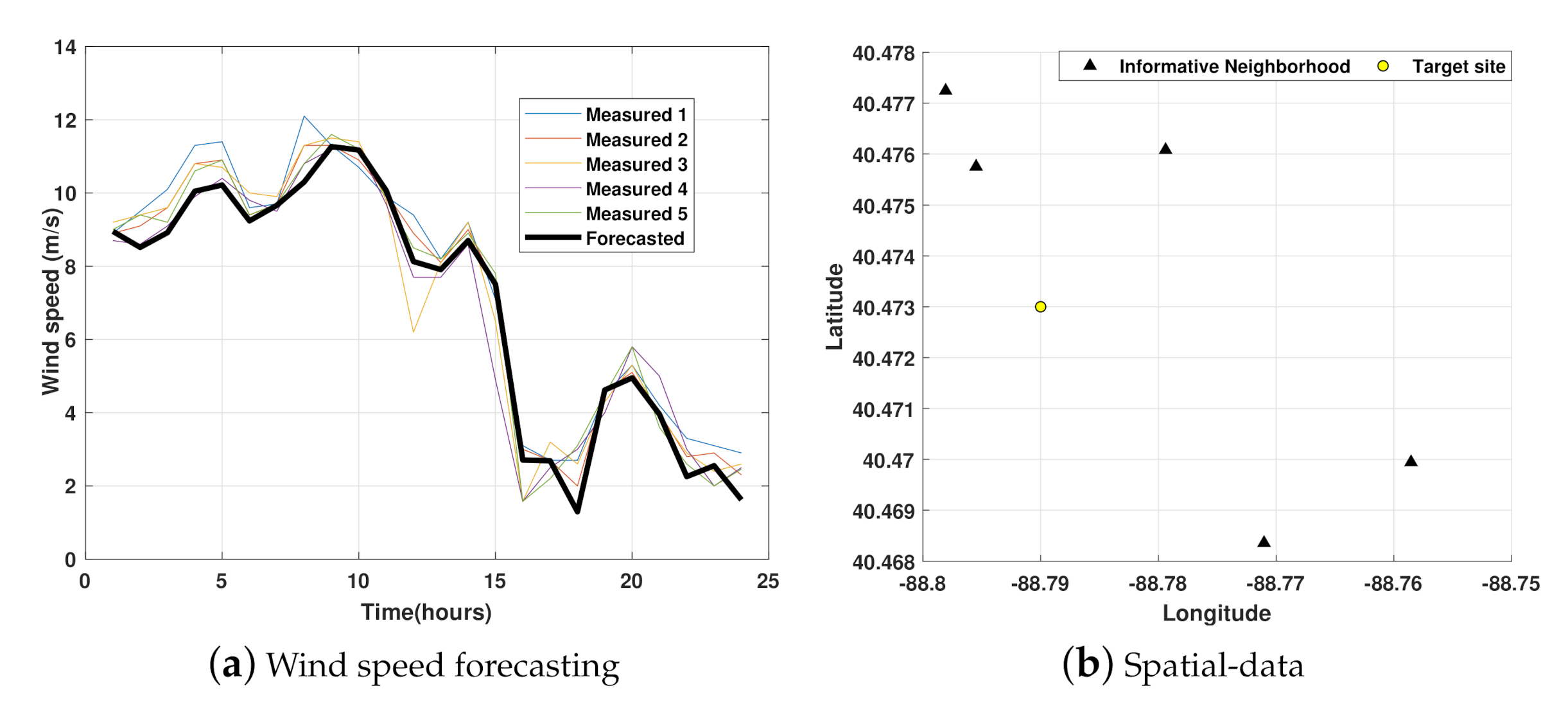
Concerning spatial-temporal modeling, a set of points (triangle) and a set of wind speeds are considered, as shown in Figure 3. Furthermore, the value of wind speed at the new location $s_0$ (circle) is required to predict.

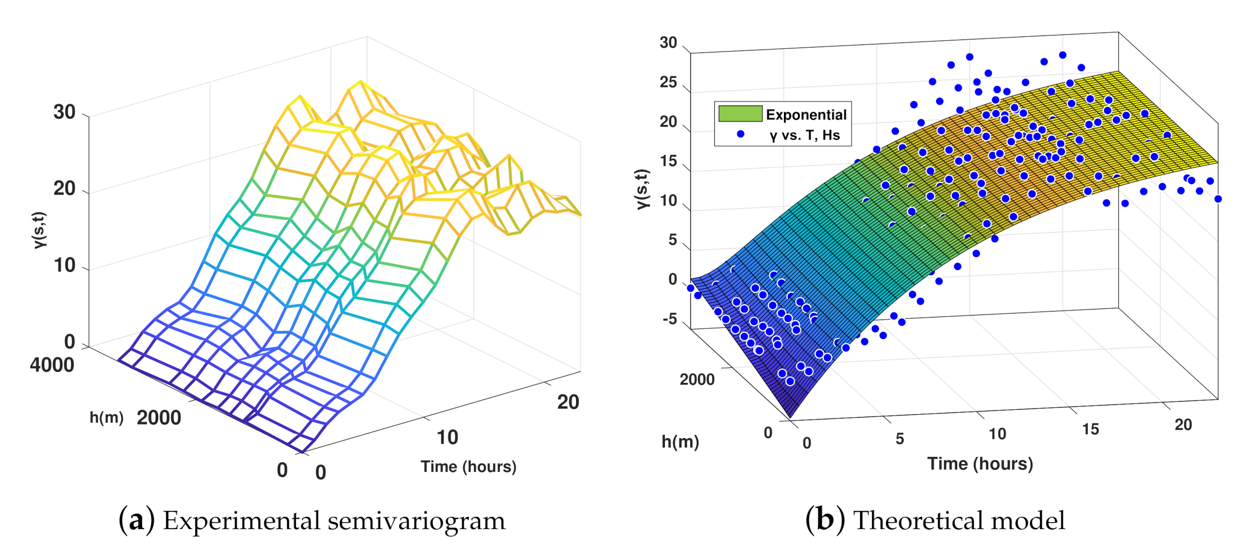
To compute the estimates, the spatial and temporal distances to be used for the construction of the semivariogram are calculated. Next, the experimental semivariogram based on Equation (17) is developed in order to establish a theoretical model for the covariance function between the spatial-temporal data. Once the semivariogram has been constructed, the data are adjusted to the theoretical model. Based on the adjustment made, it was decided that the most acceptable model was the exponential curve. Figure 4 depicts the experimental semivariogram and the model fitted.

The corresponding exponential covariance function has the form that can be defined by:

$$C(h_s,h_t)=c_0+c_1\left(1-e^{-\frac{\sqrt{h_s^2+{\left(\kappa h_t\right)}^2}}{a}}\right)$$

(55)

where $c_0$, $c_1$, k, and a are parameters obtained by the fitting and h and u are spatial and temporal data, respectively.

Once the model of the semivariogram is adjusted, the kriging weights are calculated by solving Equation (52):

$$\lambda i=\left[\begin{array}{c}-1.177\\ 2.053\\ -0.003\\ 0.172\\ -0.047\end{array}\right]$$

(56)

Note that the weights sum to one.

Now the predicted value of Z at the unobserved point can be calculated by (53). Figure 5 depicts the prediction developed (black line) at the unobserved point.

The next step is to use the Monte Carlo, ARMA, and spatio-temporal methods to generate several scenarios for each hour of the next 24 h. Once the wind scenarios are generated, the Kantorovich distance algorithm is used to reduce the number of realizations. It should be taken into account that the sum of the probabilities for both the complete set of scenarios and the reduced set is always one. Figure 6 depicts the reduced scenarios (only 10 scenarios are shown). From this set, wind power scenarios are derived. Equation (5) is used to calculate the output power.

Statistical analysis metrics are used to discuss the performance of the scenario: the mean, mean absolute error, and root mean squared error are evaluated.

Table 2. Forecast error statistics.

Method	Mean	MAE	RMSE
ARMA model	7.613	0.314	1.079
Monte Carlo	7.599	0.312	1.103
Spatio-temporal	7.164	0.284	0.934

shows the forecast error statistics for the methods. The overall error characteristics were calculated using two values: the mean absolute error (MAE) and the root-mean squared error (RMSE). In Table 2, it can be seen that the scenarios based on the spatio-temporal model have lower error values.

To evaluate the computational cost, the three methods were used to generate 300 scenarios. All computational tests were conducted using MATLAB 9.2 on a desktop with a Core-i7 processor, 2.60 gigahertz, 12 gigabytes RAM, and GPU GeForce GTX 960M. The ARMA method generates scenarios from an ARMA model derived from the database and uses the parameters k and c of the associated Weibull distribution. The total computer time for ARMA is 1.183 s. The Monte Carlo method generates scenarios using the parameters k and c of the Weibull distribution. The total computer time for Monte Carlo is 0.298 s. Finally, the spatio-temporal method generates scenarios through the kriging model and analogs in the database. The total computer time for spatio-temporal method is 8.981 s.

The results demonstrate that the proposed algorithms generate scenarios that fit appropriately to the database used. Based on the forecast error statistics, it can be verified that the scenarios based on the spatio-temporal and analog method have better performance. Finally, the Monte Carlo approach provides lower computational costs and a reduced number of parameters for the generation of scenarios.

4.3. ED Results

The modified IEEE-3 bus and IEEE-24 test systems are proposed for the study of the ED problem with the use of spatio-temporal kriging and common methods for modeling the generation of wind.

The ED model was implemented in the Julia programming environment, and the simulations were performed on a laptop with a Core-i7 processor, 2.60 gigahertz, 12 gigabytes RAM, and GPU GeForce GTX 960M.

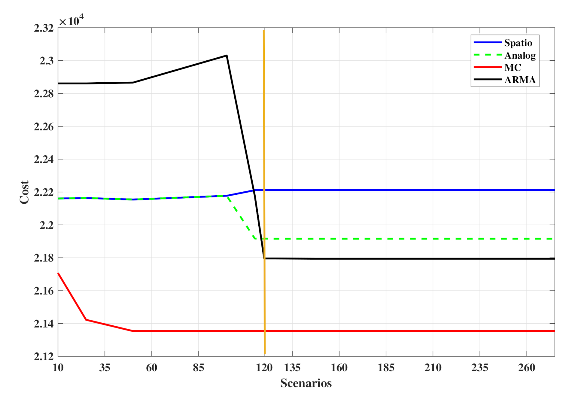
In order to analyze and compare the impact of different scenarios, a test was performed to determine the appropriate number of scenarios to use in the dispatch problem by increasing the number of scenarios and observing the behavior of the objective function. The corresponding numerical results obtained are shown in Figure 7, where the value of the cost function for each method and the corresponding number of scenarios are depicted. For a set of scenarios less than 120, the cost function has variations, while for values greater than 120, it can be verified that the changes in the value of the objective function are negligible. Based on results of the figure, it can be established that a set of 120 scenarios is adequate for uncertainty assessment due to renewable generation.

The methods are compared in two aspects: costs of dispatch and computational time.

4.4. Case 1: IEEE-3 Bus Test System

The modified IEEE-3 bus test system is used to demonstrate the effectiveness of proposed method. The system has three conventional power plants located in bus 1, bus 2, and bus 3 and one wind generator located in bus 2, as shown in Figure 8. All technical specifications for the generation units and the test system were reported in [54]. The installed capacity of the wind farm is 30 MW for this case. The penalty coefficient $\alpha$ (underestimation cost coefficient) for wind curtailment is 80 $/MW, and the penalty coefficient $\beta$ (overestimation cost coefficient) for load shedding is 160 $/MW [10]. The maximum allowable load shedding percentage $\gamma$ is set to be $5\%$ [10].

The total cost of the methods after running the optimization problem described in Section 2.3 by Equations (35)–(42), for an arbitrary selected day, are listed in

Table 3. The costs of methods.

Method	Initial Costs ($)	Ex-Post Costs ($)
DO	47,265.129	50,984.885
ARMA model	48,891.282	40,502.540
Monte Carlo	47,684.425	42,168.046
Spatio-temporal	47,735.511	39,971.381

. The table details the cost of dispatch before and after the actual wind power. As shown, the cost of the deterministic approach (DO) is lower than that of the other methods before the real wind power is dispatched. However, with actual wind power, it is found that the cost of the spatio-temporal method is lower than the deterministic, Monte Carlo, and ARMA costs. This demonstrates that scenario based methods perform better than deterministic ones in the presence of uncertainty. In general, the proposed method has better overall savings.

Table 4. Demand of the system.

	${\mathit{t}}_1$	${\mathit{t}}_2$	${\mathit{t}}_3$	${\mathit{t}}_4$	${\mathit{t}}_5$	${\mathit{t}}_6$	${\mathit{t}}_7$	${\mathit{t}}_8$	${\mathit{t}}_9$	${\mathit{t}}_{10}$
Demand (MW)	177.500	166.900	159.030	156.300	156.300	159.030	196.100	227.900	251.700	251.700

,

Table 5. Economic dispatch with ARMA scenarios.

Variable\Time	${\mathit{t}}_1$	${\mathit{t}}_2$	${\mathit{t}}_3$	${\mathit{t}}_4$	${\mathit{t}}_5$	${\mathit{t}}_6$	${\mathit{t}}_7$	${\mathit{t}}_8$	${\mathit{t}}_9$	${\mathit{t}}_{10}$
$P_1$ (MW)	78.625	68.555	60.777	58.122	58.040	61.079	96.295	126.505	150.000	150.000
$P_2$ (MW)	10.000	10.000	10.000	10.00	10.000	10.000	10.000	10.000	10.604	10.937
$P_3$ (MW)	80.000	80.00	80.000	80.000	80.000	80.000	80.00	80.000	80.000	80.000
Wind (MW)	8.875	8.345	8.253	8.178	8.259	7.952	9.805	11.395	11.096	10.763

,

Table 6. Economic dispatch with spatio-temporal scenarios.

Variable\Time	${\mathit{t}}_1$	${\mathit{t}}_2$	${\mathit{t}}_3$	${\mathit{t}}_4$	${\mathit{t}}_5$	${\mathit{t}}_6$	${\mathit{t}}_7$	${\mathit{t}}_8$	${\mathit{t}}_9$	${\mathit{t}}_{10}$
$P_1$ (MW)	78.625	68.555	61.079	58.485	58.485	61.079	96.295	126.505	149.115	149.115
$P_2$ (MW)	10.000	10.000	10.000	10.000	10.000	10.000	10.000	10.000	10.000	10.000
$P_3$ (MW)	80.000	80.000	80.000	80.000	80.000	80.000	80.000	80.000	80.000	80.000
Wind (MW)	8.875	8.345	7.952	7.815	7.815	7.952	9.805	11.395	12.585	12.585

and

Table 7. Economic dispatch with Monte Carlo scenarios.

Variable\Time	${\mathit{t}}_1$	${\mathit{t}}_2$	${\mathit{t}}_3$	${\mathit{t}}_4$	${\mathit{t}}_5$	${\mathit{t}}_6$	${\mathit{t}}_7$	${\mathit{t}}_8$	${\mathit{t}}_9$	${\mathit{t}}_{10}$
$P_1$ (MW)	78.625	71.661	61.079	58.654	58.485	63.801	99.035	133.912	150.000	150.000
$P_2$ (MW)	10.00 0	10.000	10.000	10.000	10.000	10.000	10.000	10.000	10.874	13.714
$P_3$ (MW)	80.000	80.000	80.000	80.000	80.000	80.000	80.000	80.000	80.000	80.000
Wind (MW)	8.875	5.239	7.952	7.646	7.815	5.229	7.065	3.988	10.826	7.987

present the results of the economic dispatch under the proposed model for the different alternatives. When all values of $P_{g,t}$ and $Wind$ are summed, they meet the necessary demand at t. The generation costs of generators $P_1$, $P_2$, and $P_3$ are 30 $, 40 $, and 20 $. The maximum capacity of the generators is 150 MW, 150 MW, and 80 MW, respectively. It is observed that the most economical generators $P_1$ and $P_3$ are those that participate mainly in the dispatch for all cases. In all three cases, generator $P_2$, which is the most expensive, dispatches its minimum capacity. Furthermore, generator $P_3$, which is the least expensive, dispatches its maximum capacity. The tables also present the amount of wind power used to complete the dispatch. For this case study, when using the ARMA method, four-point-nine percent of the total demand is met with wind and in the case of spatio-temporal 5% and for Monte Carlo 3.8%.

The computational time of methods are listed in

Table 8. The computation time of the methods.

Method	Time (s)
DO	18.975
ARMA model	30.688
Monte Carlo	31.720
Spatio-temporal	33.221

. For the DOmethod, the computation time is about 18.975 s, for the spatio-temporal about 33.221 s, for Monte Carlo about 31.720 s, and for the ARMA model about 30.688 s. The computation time of the spatio-temporal method is longer than that of the deterministic, ARMA, and Monte Carlo based methods.

4.5. Case 2: IEEE-24 Bus Test System

The modified IEEE-24 bus test system, shown in Figure 9, is used with twelve conventional generators and one wind generator located in bus 3. All technical specifications for the generation units and the test system were reported in [55]. The installed capacity of the wind farm is 500 MW for this case. The penalty coefficient $\alpha$ (underestimation cost coefficient) for wind curtailment is 80 $/MW, and the penalty coefficient $\beta$ (overestimation cost coefficient) for load shedding is 160 $/MW [10]. The maximum allowable load shedding percentage $\gamma$ is set to be $5\%$ [10].

The total cost of the methods after running the optimization problem described in Section 2.3 in Equations (35)–(42), for an arbitrary selected day, are listed in

Table 9. The costs of the methods.

Method	Initial Costs ($)	Ex-Post Costs ($)
DO	324,281.956	580,689.927
ARMA model	617,789.669	577,629.647
Monte Carlo	635,792.068	581,598.627
Spatio-temporal	594,790.979	576,376.125

. As shown, the cost of the deterministic approach is lower than that of the other methods before the real wind power is dispatched. However, with actual wind power, it is found that the cost of the spatio-temporal method is lower than the deterministic, Monte Carlo, and ARMA costs.

The computational time of methods are listed in

Table 10. The computation time of the methods.

Method	Time (s)
DO	23.229
ARMA model	448.288
Monte Carlo	410.833
Spatio-temporal	429.401

. For the DO method, the computation time is about 23.229 s, for the spatio-temporal about 429.401 s, for Monte Carlo about 410.833 s, and for the ARMA model about 448.288 s. The computation time of the spatio-temporal method is longer than that of the deterministic and Monte Carlo methods and shorter than that of ARMA based method.

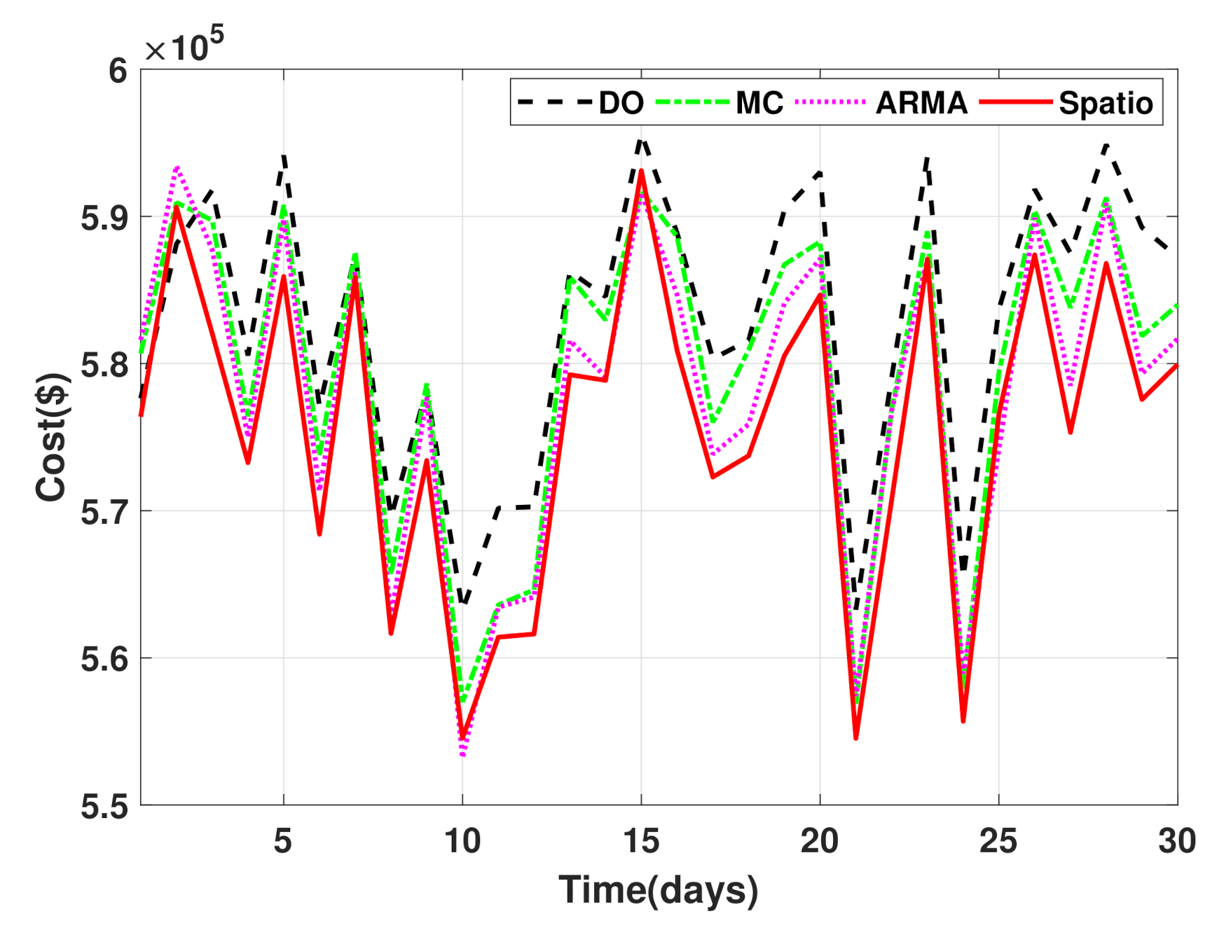
Finally, an estimation of the behavior of the total cost of the ED problem is carried out over 30 days. Figure 10 depicts the cost behavior for the DO (black), Monte Carlo (green), ARMA (magenta), and spatio-temporal (red) approaches. The scenario based approaches are found to have a lower cost than the deterministic method under uncertainty.

Figure 10 depicts that the spatio-temporal method has the lowest costs most of the days tested. However, there are also points, as in $t_{10}$, where the ARMA method has the lowest cost.

Table 11. Average costs.

	DO	Monte Carlo	ARMA	Spatio-Temporal
Average ($)	582,840.000	579,740.000	577,970.000	575,670.000
%	-	0.532	0.836	1.230

reports the average total cost of each case and also indicates, in percentage, the cost decrease obtained when compared to the deterministic method.

As seen in Table, with the spatio-temporal approach, the highest percentage of cost reduction (1.230%) is achieved.

5. Conclusions

This research examined three wind scenario creation methods. The methods allow the operator to leverage historical data to create many scenarios. Furthermore, this paper describes a wind prediction model using a spatio-temporal model based on the kriging method. From the spatio-temporal prediction, wind scenarios are generated using analogs. These scenarios are then converted into wind power, considering the power curve of the wind turbines. An economic dispatch model is then established so that the generated scenarios can be integrated into the formulation. Finally, the problem is implemented and evaluated on modified IEEE 3-bus and IEEE 24-bus systems. The following conclusions are established based on the studies:

• The proposed approach for spatio-temporal modeling has a better fit for the database than the ARMA and Monte Carlo methods. Therefore, it can be applied to predict the values on unobserved points from data measured around the unmeasured point. In this work, the data of the wind speed and the location of these measurements are used. It can also be mentioned that when the scenarios are generated, the Monte Carlo method is the one with the lowest computational cost. At the same time, the spatio-temporal approach has the highest cost.
• Because the weights of the kriging estimator depend on the modeled semivariogram, kriging is very sensitive to the misspecification of the semivariogram model.
• In general, interpolation accuracy by kriging is limited if the number of observations sampled is small. The data are limited in spatial scope, or the data are not broadly spatially correlated. In these cases, it is challenging to generate an experimental semivariogram.
• The number of scenarios is an important parameter and can have a significant impact on the cost function of the ED problem. A good value for $N_s$ is likely to depend on the method of scenario creation. For the presented approach, the stabilization of the objective function occurred in values close to 120 scenarios, as can be seen in Figure 7.
• An economic dispatch model that considers wind generation in its formulation is presented in this research. Wind generation is created using a kriging based spatio-temporal model and other methods commonly used for this purpose. The proposed approach’s effectiveness is demonstrated by the simulation of the modified IEEE 3-bus and IEEE-24 bus systems.
• The results show that spatio-temporal and analog models for generating scenarios can be integrated efficiently in the ED problem framework and reduce costs. The reduction in operating costs when using spatio-temporal scenarios is 1.230%.

Scenario creation and ED problem under uncertainty remains an open area for research. Many of the methods presented in this paper could be improved upon to produce better scenarios and to attain ED solutions with lower costs in less time. Scenario creation methods have the potential to be applied to other sources of uncertainty in the power system. We can further take advantage of spatio-temporal and analog based approaches and provide different strategies for modeling uncertainties on both the supply and demand sides. Finally, savings due to ED under uncertainty are likely to vary from system-to-system and with wind energy penetration. The number of scenarios used may play a large role in the dispatch costs. Evaluations of the potential for savings should be made for other systems, especially those with flexibility requirements. Further work will focus on the application in a real power grid.

References

1. Jiang, C.; Chen, Y.; Mao, Y.; Chai, Y.; Yu, M. Forecasting Spatio-Temporal Renewable Scenarios: A Deep Generative Approach. arXiv 2019, arXiv:1903.05274. [Google Scholar]
2. Le, D.D.; Gross, G.; Berizzi, A. Probabilistic modeling of multisite wind farm production for scenario based applications. IEEE Trans. Sustain. Energy 2015, 6, 748–758. [Google Scholar] [CrossRef] [Green Version]
3. Xie, L.; Gu, Y.; Zhu, X.; Genton, M.G. Short-Term Spatio-Temporal Wind Power Forecast in Robust Look-ahead Power System Dispatch. IEEE Trans. Smart Grid 2014, 5, 511–520. [Google Scholar] [CrossRef]
4. Meibom, P.; Barth, R.; Hasche, B.; Brand, H.; Weber, C.; O’Malley, M. Stochastic optimization model to study the operational impacts of high wind penetrations in Ireland. IEEE Trans. Power Syst. 2011, 26, 1367–1379. [Google Scholar] [CrossRef]
5. Yıldız, C.; Tekin, M.; Gani, A.; Keçecioğlu, Ö.; Açıkgöz, H.; Şekkeli, M. A Day-Ahead Wind Power Scenario Generation, Reduction, and Quality Test Tool. Sustainability 2017, 9, 864. [Google Scholar] [CrossRef] [Green Version]
6. Camal, S.; Teng, F.; Michiorri, A.; Kariniotakis, G.; Badesa, L. Scenario generation of aggregated Wind, Photovoltaics and small Hydro production for power systems applications. Appl. Energy 2019, 242, 1396–1406. [Google Scholar] [CrossRef] [Green Version]
7. Du, E.; Zhang, N.; Kang, C.; Xia, Q. Scenario Map Based Stochastic Unit Commitment. IEEE Trans. Power Syst. 2018, 33, 4694–4705. [Google Scholar] [CrossRef]
8. Ming, H.; Xie, L.; Campi, M.C.; Garatti, S.; Kumar, P.R. Scenario-Based Economic Dispatch With Uncertain Demand Response. IEEE Trans. Smart Grid 2019, 10, 1858–1868. [Google Scholar] [CrossRef] [Green Version]
9. Modarresi, M.S.; Xie, L.; Campi, M.C.; Garatti, S.; Care, A.; Thatte, A.A.; Kumar, P.R. Scenario-Based Economic Dispatch With Tunable Risk Levels in High-Renewable Power Systems. IEEE Trans. Power Syst. 2019, 34, 5103–5114. [Google Scholar] [CrossRef]
10. Xu, J.; Wang, B.; Sun, Y.; Xu, Q.; Liu, J.; Cao, H.; Jiang, H.; Lei, R.; Shen, M. A day-ahead economic dispatch method considering extreme scenarios based on a wind power uncertainty set. CSEE J. Power Energy Syst. 2019. [Google Scholar] [CrossRef]
11. Sandelic, M.; Stroe, D.I.; Iov, F. Battery Storage-Based Frequency Containment Reserves in Large Wind Penetrated Scenarios: A Practical Approach to Sizing. Energies 2018, 11, 3065. [Google Scholar] [CrossRef] [Green Version]
12. Valizadeh Haghi, H.; Bina, M.T.; Golkar, M.A. Nonlinear modeling of temporal wind power variations. IEEE Trans. Sustain. Energy 2013, 4, 838–848. [Google Scholar] [CrossRef]
13. Salehi Borujeni, M.; Akbari Foroud, A.; Dideban, A. Wind speed scenario generation based on dependency structure analysis. J. Wind Eng. Ind. Aerodyn. 2018, 172, 453–465. [Google Scholar] [CrossRef]
14. Ezzat, A.A.; Jun, M.; Ding, Y. Spatio-temporal asymmetry of local wind fields and its impact on short-term wind forecasting. IEEE Trans. Sustain. Energy 2018, 9, 1437–1447. [Google Scholar] [CrossRef] [PubMed]
15. Xie, L.; Gu, Y.; Zhu, X.; Genton, M.G. Power system economic dispatch with spatio-temporal wind forecasts. In Proceedings of the IEEE 2011 EnergyTech, Cleveland, OH, USA, 25–26 May 2011; pp. 1–6. [Google Scholar] [CrossRef]
16. Xie, L.; Gu, Y.; Zhu, X.; Genton, M. Short-term spatio-temporal wind power forecast in robust look-ahead power system dispatch. In Proceedings of the 2016 IEEE Power and Energy Society General Meeting (PESGM), Boston, MA, USA, 17–21 July 2016; p. 1. [Google Scholar] [CrossRef]
17. Tascikaraoglu, A.; Sanandaji, B.M.; Chicco, G.; Cocina, V.; Spertino, F.; Erdinc, O.; Paterakis, N.G.; Catalao, J.P.S. A short-term spatio-temporal approach for Photovoltaic power forecasting. In Proceedings of the 2016 Power Systems Computation Conference (PSCC), Genoa, Italy, 20–24 June 2016; pp. 1–7. [Google Scholar] [CrossRef]
18. Zhao, Y.; Ye, L.; Wang, Z.; Wu, L.; Zhai, B.; Lan, H.; Yang, S. Spatio-temporal Markov chain model for very-short-term wind power forecasting. J. Eng. 2019, 2019, 5018–5022. [Google Scholar] [CrossRef]
19. Sun, M.; Feng, C.; Zhang, J. Conditional aggregated probabilistic wind power forecasting based on spatio-temporal correlation. Appl. Energy 2019, 256, 113842. [Google Scholar] [CrossRef]
20. Suryawanshi, A.; Ghosh, D. Wind speed prediction using spatio-temporal covariance. Nat. Hazards 2015, 75, 1435–1449. [Google Scholar] [CrossRef]
21. Agoua, X.G.; Girard, R.; Kariniotakis, G. Probabilistic Models for Spatio-Temporal Photovoltaic Power Forecasting. IEEE Trans. Sustain. Energy 2019, 10, 780–789. [Google Scholar] [CrossRef] [Green Version]
22. Zhu, Q.; Chen, J.; Zhu, L.; Duan, X.; Liu, Y. Wind Speed Prediction with Spatio–Temporal Correlation: A Deep Learning Approach. Energies 2018, 11, 705. [Google Scholar] [CrossRef] [Green Version]
23. Hama, K.; Fujimoto, Y.; Hayashi, Y. Expected Wind Speed Estimation Considering Spatio-Temporal Anisotropy for Generating Synthetic Wind Power Profiles. Energy Procedia 2018, 155, 309–319. [Google Scholar] [CrossRef]
24. Dowell, J.; Weiss, S.; Hill, D.; Infield, D. Short-term spatio-temporal prediction of wind speed and direction. Wind Energy 2014, 17, 1945–1955. [Google Scholar] [CrossRef]
25. Dowell, J.; Weiss, S.; Infield, D. Kernel methods for short-term spatio-temporal wind prediction. In Proceedings of the 2015 IEEE Power & Energy Society General Meeting, Denver, CO, USA, 26–30 July 2015; Volume 2015, pp. 1–5. [Google Scholar] [CrossRef] [Green Version]
26. Khodayar, M.; Wang, J. Spatio-Temporal Graph Deep Neural Network for Short-Term Wind Speed Forecasting. IEEE Trans. Sustain. Energy 2019, 10, 670–681. [Google Scholar] [CrossRef]
27. Agoua, X.G.; Girard, R.; Kariniotakis, G. Short-Term Spatio-Temporal Forecasting of Photovoltaic Power Production. IEEE Trans. Sustain. Energy 2018, 9, 538–546. [Google Scholar] [CrossRef] [Green Version]
28. Aryaputera, A.W.; Yang, D.; Zhao, L.; Walsh, W.M. Very short-term irradiance forecasting at unobserved locations using spatio-temporal kriging. Sol. Energy 2015, 122, 1266–1278. [Google Scholar] [CrossRef]
29. Jamaly, M.; Kleissl, J. Spatiotemporal interpolation and forecast of irradiance data using Kriging. Sol. Energy 2017, 158, 407–423. [Google Scholar] [CrossRef]
30. Hu, Q.; Chen, H.; Tao, Y.; Yang, R.; Wang, L.; Hu, P. Wind speed spatio-temporal forecasting of wind farms based on universal kriging and Bayesian dynamic model. In Proceedings of the 2014 International Conference on Power System Technology, Chengdu, China, 20–22 October 2014; pp. 2897–2902. [Google Scholar] [CrossRef]
31. He, M.; Yang, L.; Zhang, J.; Vittal, V. Spatio-temporal analysis for smart grids with wind generation integration. In Proceedings of the 2013 International Conference on Computing, Networking and Communications (ICNC), San Diego, CA, USA, 28–31 January 2013; pp. 1107–1111. [Google Scholar] [CrossRef]
32. Lenzi, A.; Steinsland, I.; Pinson, P. Spatio-temporal modeling for short term wind power forecasts. Why, when and how. In Proceedings of the EGU General Assembly Conference Abstracts, Vienna, Austria, 23–28 April 2017; p. 3633. [Google Scholar]
33. Filik, T. Improved Spatio-Temporal Linear Models for Very Short-Term Wind Speed Forecasting. Energies 2016, 9, 168. [Google Scholar] [CrossRef] [Green Version]
34. Lorca, A.; Sun, X.A. Adaptive Robust Optimization With Dynamic Uncertainty Sets for Multi-Period Economic Dispatch Under Significant Wind. IEEE Trans. Power Syst. 2015, 30, 1702–1713. [Google Scholar] [CrossRef] [Green Version]
35. Bessa, R.J.; Trindade, A.; Miranda, V. Spatial-temporal solar power forecasting for smart grids. IEEE Trans. Ind. Inform. 2015, 11, 232–241. [Google Scholar] [CrossRef]
36. He, X.D.; Cui, C.G.; Yang, N. The Kriging model based scenario generation and its application in the energy internet with high wind penetration. In Proceedings of the 2017 IEEE Conference on Energy Internet and Energy System Integration (EI2), Beijing, China, 26–28 November 2017; pp. 1–6. [Google Scholar] [CrossRef]
37. Tascikaraoglu, A.; Sanandaji, B.M. Short-term residential electric load forecasting: A compressive spatio-temporal approach. Energy Build. 2016, 111, 380–392. [Google Scholar] [CrossRef]
38. Zhu, X.; Genton, M.G.; Gu, Y.; Xie, L. Space-time wind speed forecasting for improved power system dispatch. Test 2014, 23, 1–25. [Google Scholar] [CrossRef]
39. Fan, F.; Bell, K.; Hill, D.; Infield, D. Wind forecasting using kriging and vector auto-regressive models for dynamic line rating studies. In Proceedings of the 2015 IEEE Eindhoven PowerTech, Eindhoven, The Netherlands, 29 June–2 July 2015; pp. 1–6. [Google Scholar] [CrossRef] [Green Version]
40. Tang, J.; Wang, D.; Wang, X.; Jia, H.; Wang, C.; Huang, R.; Yang, Z.; Fan, M. Study on day-ahead optimal economic operation of active distribution networks based on Kriging model assisted particle swarm optimization with constraint handling techniques. Appl. Energy 2017, 204, 143–162. [Google Scholar] [CrossRef]
41. van Stein, B.; Wang, H.; Kowalczyk, W.; Emmerich, M.; Bäck, T. Cluster based Kriging approximation algorithms for complexity reduction. Appl. Intell. 2020, 50, 778–791. [Google Scholar] [CrossRef] [Green Version]
42. Strandberg, J.; Sjöstedt de Luna, S.; Mateu, J. Prediction of spatial functional random processes: Comparing functional and spatio-temporal kriging approaches. Stoch. Environ. Res. Risk Assess. 2019, 33, 1699–1719. [Google Scholar] [CrossRef] [Green Version]
43. Analui, B.; Scaglione, A. An approximation algorithm for future wind scenarios. In Proceedings of the 2016 IEEE Statistical Signal Processing Workshop (SSP), Palma de Mallorca, Spain, 26–29 June 2016; pp. 1–5. [Google Scholar] [CrossRef]
44. Pishgar-Komleh, S.; Keyhani, A.; Sefeedpari, P. Wind speed and power density analysis based on Weibull and Rayleigh distributions (a case study: Firouzkooh county of Iran). Renew. Sustain. Energy Rev. 2015, 42, 313–322. [Google Scholar] [CrossRef]
45. Sharma, K.C.; Jain, P.; Bhakar, R. Wind Power Scenario Generation and Reduction in Stochastic Programming Framework. Electr. Power Components Syst. 2013, 41, 271–285. [Google Scholar] [CrossRef]
46. Chen, J.; Rabiti, C. Synthetic wind speed scenarios generation for probabilistic analysis of hybrid energy systems. Energy 2017, 120, 507–517. [Google Scholar] [CrossRef] [Green Version]
47. Ding, Y. Data Science for Wind Energy; Chapman and Hall, CRC: Boca Raton, FL, USA, 2019. [Google Scholar] [CrossRef]
48. Varouchakis, E.A.; Hristopulosb, D.T. Comparison of spatiotemporal variogram functions based on a sparse dataset of groundwater level variations. Spat. Stat. 2019, 34, 100245. [Google Scholar] [CrossRef]
49. Xu, J.; Shu, H. Spatio-temporal kriging based on the product-sum model: Some computational aspects. Earth Sci. Inform. 2015, 8, 639–648. [Google Scholar] [CrossRef]
50. Li, W.; Duan, Q.; Miao, C.; Ye, A.; Gong, W.; Di, Z. A review on statistical postprocessing methods for hydrometeorological ensemble forecasting. Wiley Interdiscip. Rev. Water 2017, 4, e1246. [Google Scholar] [CrossRef]
51. Ben Daoud, A.; Sauquet, E.; Bontron, G.; Obled, C.; Lang, M. Daily quantitative precipitation forecasts based on the analogue method: Improvements and application to a French large river basin. Atmos. Res. 2016, 169, 147–159. [Google Scholar] [CrossRef] [Green Version]
52. Morales, J.M.; Zugno, M.; Pineda, S.; Pinson, P. Electricity market clearing with improved scheduling of stochastic production. Eur. J. Oper. Res. 2014, 235, 765–774. [Google Scholar] [CrossRef] [Green Version]
53. Carrillo, C.; Obando Montaño, A.F.; Cidrás, J.; Díaz-Dorado, E. Review of power curve modelling for wind turbines. Renew. Sustain. Energy Rev. 2013, 21, 572–581. [Google Scholar] [CrossRef]
54. Gazafroudi, A.S.; Shafie-khah, M.; Prieto-Castrillo, F.; Talari, S.; Corchado, J.M.; Catalão, J.P. Evolving New Market Structures. Pathways Smarter Power Syst. 2019, 183–203. [Google Scholar] [CrossRef]
55. Ordoudis, C.; Pinson, P.; González, J.M.M.; Zugno, M. An Updated Version of the IEEE RTS 24-Bus System for Electricity Market and Power System Operation Studies; Technical University of Denmark: Kgs. Lyngby, Denmark, 2016; pp. 1–6. [Google Scholar]
Figure 1. Solution methodology flowchart.
Energies 13 06419 g001
Figure 2. Spatio-temporal distances.
Energies 13 06419 g002
Figure 3. Spatio-temporal wind speed data. (a) depicts the wind speed data at measured points. (b) depicts the coordinates of the measured points and the target site.
Energies 13 06419 g003
Figure 4. Experimental semivariogram and theoretical model of spatio-temporal data. (a) depicts the semivariogram obtained from spatio-temporal data. (b) depicts the fit of the experimental semivariogram to the theoretical model.
Energies 13 06419 g004
Figure 5. Spatio-temporal wind speed data. (a) depicts the wind speed measured data, and the wind speed forecasted. (b) depicts the coordinates of the measured points and the target site.
Energies 13 06419 g005
Figure 6. Wind speed scenarios. (a) depicts the wind speed scenarios generated by the ARMA method. (b) depicts the wind speed scenarios generated by the Spatio-temporal method. (c) depicts the wind speed scenarios generated by the Monte Carlo method.
Energies 13 06419 g006
Figure 7. Changes in the objective function value vs. the number of scenarios.
Energies 13 06419 g007
Figure 8. IEEE-3 bus test system.
Energies 13 06419 g008
Figure 9. IEEE-24 bus test system.
Energies 13 06419 g009
Figure 10. Dispatched ED costs.
Energies 13 06419 g010