Article

Study on Asymmetry Concentration of Mixed Oil in Products Pipeline

1
National Engineering Laboratory for Pipeline Safety, China University of Petroleum, Beijing 102249, China
2
MOE Key Laboratory of Petroleum Engineering, China University of Petroleum, Beijing 102249, China
3
Beijing Key Laboratory of Urban Oil and Gas Distribution Technology, China University of Petroleum, Beijing 102249, China
4
Department of Applied Physics, Universitat Politècnica de Catalunya, 08034 Barcelona, Spain
*
Author to whom correspondence should be addressed.
Energies 2020, 13(23), 6398; https://doi.org/10.3390/en13236398
Submission received: 22 October 2020 / Revised: 1 December 2020 / Accepted: 1 December 2020 / Published: 3 December 2020

Abstract

:
Long-distance pipelines transporting multiple product oils such as gasoline, diesel and jet fuel, are important facilities for transporting fossil energy. One major concern in operation is the energy consumption of the pipeline. Energy consumption should be made optimized tracking batches of oils and cutting mixed oil, which requires an accurate prediction of concentration curve. In engineering, the concentration curve is usually assumed to be symmetric, but it is actually asymmetric, which may lead to estimation errors. Thus, the asymmetric concentration of mixed oil should be studied. The formation mechanism of the asymmetry of concentration curve has not been clearly clarified. A new method is proposed to measure the asymmetry of the concentration curve. Quantitative analysis is carried out for each factor on the asymmetry distribution of concentration curve. Based on the convection–diffusion equation, a modified oil-mixing model considering near wall adsorption effect is established. The model shows a good agreement with the Jablonski empirical formula. The error, compared with the experimental results, is less than 5%. The main findings are: (1) deviation volume has a negative correlation with pipe diameter and mean velocity; (2) adsorption coefficient has a greater impact on the length ratio of front and tail oil than diffusion coefficient; (3) the influence of all factors considered on the total length of mixed oil, front oil, tail oil and trail oil are basically the same; (4) if the limit of adsorption concentration in adsorption layer is 1, the reasonable value of adsorption coefficient a and b should be around 0.4. The results reveal the mechanism of asymmetric concentration of product oils and can provide practical suggestions to deal with the mixed oil.

1. Introduction

An efficient way to transport different types of product oils over a long distance is to use one pipeline to transport the different oils sequentially because the construction of multiple pipelines would require much larger investments and energy consumption. Consecutive oils in pipeline form one interfacial section containing mixed oil [1]. A long-distance pipeline has several mixed oil sections. Oil transportation enterprises require the mixed oil sections to be as few and short as possible, to ensure a high-quality product. This requires scheduling, batch interface tracking and mixed oil cutting in engineering. The complexity of these operations increase with the increasing types of product oil and the branch points [2]. Due to the high efficiency of computer-aided programming of this complex problem, the requirements for numerical simulation of mixed oil flow in products pipelines have gradually increased [3]. As the positions of the front oil and tailing oil cannot be accurately obtained during the operation of the products’ pipeline, the mixing situation of the oils is difficult to obtain quickly and accurately. This results in the predicted value of the oil quality differing greatly from the actual value, which deeply affects the automated operation of the product pipeline [4].
Due to the non-uniform distribution of flow velocity on the pipe cross-section and the adsorption of oil molecules on the pipe wall, the oil-mixing concentration curve is usually asymmetrical, which greatly affects the accuracy of mixed oil cutting. The asymmetry of the oil concentration was observed by early scholars in experiments, but it can hardly be predicted accurately [5]. With the rapid developments of computers, an increasing number of scholars choose to study the mixed oil problems through numerical simulations to obtain the asymmetric phenomena of the mixed oil concentration [6]. However, the formation mechanism of the asymmetric concentration has not been revealed. With the increasing requirements of product pipeline scheduling [7] and mixed oil cutting [8], it is very important in practical operation to predict the mixed oil concentration curve quickly and accurately [9]. The fast prediction depends on an efficient mathematical model reflecting the asymmetry of oil concentration. If oil flow is treated as a one-dimensional flow, the variation in oil concentration can only be considered along the axis of the pipeline. It cannot describe the asymmetry of oil concentration in radius direction. Therefore, mathematical models of asymmetric distribution of mixed oil should be two-dimensional or three-dimensional.
Studies using two-dimensional model are summarized as follows. Lu [10] proposed a time-splitting method to decompose the two-dimensional convection–diffusion equation into a convection equation and a diffusion equation. The convection equation was solved by the characteristic line method, while the diffusion equation was solved by the finite difference method. This treatment is easy to converge. Deng and Pu [11] proposed that oil mixing was the result of the comprehensive action of radial diffusion and axial extension. The simulation results showed that the tail of mixed oil was longer than the head. The concentration of mixed oil was asymmetrically distributed. Engineering factors that affect the tailing of mixed oil were listed but the mechanism was not analyzed. Zheng and Jiang [12] and Ma and Bai [13] also found asymmetric distribution of mixed oil concentration using two-dimensional cylindrical coordinates and an adaptive grid. Wang [14] used a commercial software to establish a two-dimensional flow and mass transfer coupling model for alternating oil transportation. He analyzed the mixed oil process of gasoline as the front oil and diesel as the tailing oil in the batch transportation using numerical simulation, and obtained the relationship of the mixed oil head shape with time.
Some other scholars tried three-dimensional models. Zhao [15] established a mixed oil model based on computational fluid software by using the Reynolds time-averaged method. Simulation results show the asymmetry of the mixed oil concentration curve. In his opinion, the asymmetry is caused by flushing action of the tailing oil on the front oil, the non-uniform velocity distribution, and the initial mixed oil. Zhang [16] simulated the oil mixture and reached the conclusion that the oil mixture concentration curve is asymmetric. Wang et al. [17] considered the influence of turbulence and obtained the asymmetric concentration curve. They concluded that the cutting effect of mixed oil was better if the front oil was gasoline rather than diesel. Dai et al. [18] considered the influence of gravity on oil mixing. They found that the length of the mixed oil will increase with increasing inclination angle when diesel is in front of gasoline. When gasoline is in front of diesel, the length of mixing oil shortens with increasing inclination angle. He et al. [19] simulated the turbulent flow of gasoline and diesel in the inclined pipeline and obtained similar conclusions with Dai et al. [20].
The three-dimensional models can describe the flow details more precisely. However, they cannot be used for long-distance pipelines due to their much longer computational time compared to the two-dimensional models. Moreover, the asymmetry is mainly in the radial direction. Thus, the two-dimensional model, balancing precision and computational speed is a better choice. It is used in this paper to study the asymmetry of mixed oil concentration. From the literature review, we realize that researchers mentioned the phenomenon of the asymmetry of mixed oil concentration but did not analyze its mechanism. We are trying, in this paper, to study the asymmetry mechanism by proposing a method to measure the asymmetry and quantify the relevant influencing factors. It is very useful for guaranteeing the precise operation of multiproduct pipelines.

2. Asymmetric Distribution Model of Mixed Oil

2.1. Flow-Control Equation

The pipe flow of oils is actually three-dimensional (3D). However, oil concentration varies mainly in the radial and axial directions, and therefore the transport of the oil concentration can be considered as a two-dimensional (2D) convection–diffusion problem. The basic form of the equation is
c t + u c x = 1 r r ( r D c r ) + x ( D c x )
where, u is the flow velocity, m/s; c is the oil concentration; D is the turbulent diffusion coefficient, m2/s; r is the radial distance, m; x is the axial distance, m; t is the time, s. This equation shows the general law of convection–diffusion of oil concentrations in radial and axial directions. The left-hand side of the equation contains the partial derivative of concentration with respect to time and convection terms, while the right-hand side of the equation contains the diffusion term. In the two-dimensional model, the values of oil concentration, flow velocity and diffusion coefficient are different at the same section and different radii of the pipeline.
Since the asymmetry of oil distribution is related to the non-uniform radial distribution of velocity, Equation (1) can be expressed in different forms in different regions of the pipe cross-section. For the fully developed turbulent flow in the pipe, the flow region can be divided into a viscous sublayer, buffer layer and turbulence core, as shown in Figure 1.
The influence of convection and diffusion in different regions varies greatly, so different empirical formulas are needed to calculate the velocity field and turbulent diffusion coefficient [20]. The simplified formula for each region is as follows.
(1) Viscous sublayer
According to the no-slip boundary condition, the viscosity of the fluid near the pipe wall is extremely significant, the oil flow velocity is zero, and there is always a thin viscous sublayer on the pipe wall. This area satisfies the following conditions
y < 5 ν τ 0 / ρ
where, y is the distance from pipe wall, m; ν is the kinematic viscosity of oil, m2/s; ρ is the density of oil, kg/m3; τ 0 is the wall shear stress, Pa.
The velocity distribution in viscous sublayer is as follows
u = 2 u 0 [ 1 ( r R ) 2 ]
The diffusion mechanism is only molecular diffusion. Therefore, the diffusion coefficient D in this area can be simplified to molecular diffusion coefficient D L , i.e., D = D L . Then, the two-dimensional convective-diffusion equation is simplified as follows
c t + u c x = D L [ 1 r r ( r c r ) + 2 c x 2 ]
Equation (4) is used to calculate the oil concentration in the viscous sublayer.
(2) Buffer layer
The buffer layer refers to the transition area from the viscous sublayer to the turbulent core area. The flow area of the buffer layer is divided as follows
5 ν / ( τ 0 / ρ ) y 30 ν / ( τ 0 / ρ )
The velocity distribution in the buffer layer is as follows [21]
u = τ 0 / ρ [ 3.05 + 5.0 ln ( τ 0 / ρ y / ν ) ]
The influence of both molecular diffusion and turbulent diffusion in this area cannot be ignored. Therefore, the diffusion coefficient is taken as the sum of molecular diffusion coefficient and turbulent diffusion coefficient
D = D L + D t = ( τ 0 / ρ ( R r ) / 5 ) ν + D L
Therefore, the convection–diffusion equation in this region can be simplified to the following formula
c t + u c x = D ( 2 c r 2 + 2 c x 2 ) + 1 r [ ( R 2 r ) τ 0 / ρ 5 ν + D L ] c r
Equation (8) is the equation to calculate the oil concentration in the buffer layer.
(3) Turbulent core region
When the fluid flows turbulent in a circular tube, most of the fluids are in the turbulent core region [22], and the fluids in the above two regions only account for a small part. The turbulence core region contains the following regions [21]
y > 30 ν / ( τ 0 / ρ )
The velocity distribution in this area is as follows
u = τ 0 / ρ [ 5.5 + 2.5 ln ( τ 0 / ρ y / ν ) ]
In the turbulent core, as the turbulent diffusion is far greater than the molecular diffusion, the turbulence diffusion coefficient is about an order of magnitude greater than the molecular diffusion coefficient. Therefore, it is considered that the diffusion coefficient in the equation is equal to the turbulent diffusion coefficient, and the calculation formula is as follows
D = D t = τ 0 / ρ r ( R r ) / ( 2.5 R )
This diffusion coefficient can be substituted into Equation (1) so that the oil concentration in turbulence core region can be calculated.
For all the above equations, the initial conditions are
t = 0     x = 0 : c = 0.5 t = 0     x > 0 : c = 0
The boundary conditions are as follows
t 0     x : c = 0 t > 0     x = 0 : c = 1 t 0 : c r | r = 0 = c r | r = R = 0
where c represents the oil concentration, %; x represents the axial position of the calculated pipe section, m.

2.2. Model with Polar Adsorption Layer

The equations in Section 2.1 did not consider the adsorption effect. Diesel and gasoline can form a polar membrane on the pipe wall. The existence of the membrane is easy to cause a longer trace of the mixed oil tail. Thus, it is important to consider the polar adsorption layer in the calculation of the mixed oil concentration. The effect of adsorption is reflected by the interaction between the pipe wall and oil molecules. In the actual adsorption process, there are usually 3–4 layers of molecules in the polar adsorption layer, among which, the first layer of molecules closest to the pipe wall has the strongest adsorption capacity. For the convenience of calculation, the polar adsorption layer is considered as monolayer adsorption. The dynamic process of monolayer adsorption can be expressed by Equation (14), while the desorption process can be expressed by Equation (15)
( d c r d t ) a = K a ( 1 c r c r * ) c
where c is the oil concentration in the pipeline, %; cr is the concentration when equilibrium is reached in the polar adsorption layer; Ka is adsorption constant, s−1; cr* is the maximum concentration that can be reached in the adsorption layer without desorption, %
( d c r d t ) d = K d ( c r c r * )
where Kd represents the desorption constant, s−1.
By comprehensively considering the dynamic equilibrium process of adsorption and desorption, the following equation can be obtained
d c r d t = K a ( 1 c r c r * ) c K d ( c r c r * )
According to the assumed solution conditions, the concentration of B oil product is c; At the initial time, the adsorption concentration in the adsorption layer is 0, which can be obtained as follows
c r ( t ) = K a c r * c ( 1 e c K a + K d c r * t ) K a c + K d
It is worth noting that only when desorption does not occur can the concentration in the limiting adsorption layer reach the limit adsorption concentration cr*, where Kd = 0. When the adsorption and desorption processes occur simultaneously and reach dynamic equilibrium after a long enough time, the concentration in the adsorption layer is
c r ( ) = a c 1 + b c
where a = K a c r * K d , b = K a K d , where the values of parameters a and b are to be determined.
If the time required for adsorption and desorption to reach dynamic equilibrium is much less than the time required for oil replacement, the adsorption concentration in the polar adsorption layer is
c r = a 1 + b c c
The derivative is
d c r d c = a ( 1 + b c ) 2 > 0
Substitute Equation (20) into the convection–diffusion equation
[ 1 + a ( 1 + b c ) 2 ] c t = D 2 c x 2 u c x
The above equation is a two-dimensional model considering a single layer of polar adsorption on the pipe wall. Equation (21) can be used to calculate the oil concentration in the polar adsorption layer.

2.3. Model Considering Temperature Change

The density and viscosity of oil are related to temperature, so that temperature has an important role in batch transportation of products [23]. There is a linear relationship between the density and temperature. For liquids, in the absence of phase transitions, the higher the temperature, the less dense the liquid is. The specific conversion formula of density is as follows [5]
ρ t = ρ 20 ε ( t 20 )
where ρ t , ρ 20 are the oil density at t °C and 20 °C, kg / m 3 ; ε is the temperature coefficient ε = 1.825 0.001315 ρ 20 , Kg/(m3·°C).
The viscosity of oil at any temperatures can be obtained by converting the viscosity–temperature index of oil to the known viscosity at a certain temperature. In the absence of phase transitions, the higher the temperature, the smaller the viscosity is for a Newtonian fluid. The specific formula for viscosity conversion is as follows [5]
v t = v 0 e u ( t t 0 )
where v t represents the viscosity of the oil at t °C, m2/s; v 0 represents the viscosity of the oil at the temperature of t 0 °C, m2/s; u is the viscosity–temperature index of the oil.
The influence of temperature on Reynolds number is indirectly caused by the influence of temperature on viscosity. The influence of temperature on Reynolds number is as follows
Re = u m d ν = u m d v 0 e u ( t t 0 )
The influence of temperature on friction coefficient
λ = 0.3164 Re 0.25 = 0.3164 × ( u m d v 0 e u ( t t 0 ) ) 0.25
The influence of temperature on the shear stress of the pipe wall
τ 0 = 0.125 λ ρ u m 2 = 0 . 125 × [ 0.3164 × ( u m d v 0 e u ( t t 0 ) ) 0.25 ] × [ ρ 20 ε ( t 20 ) ] u m 2
The effect of temperature on the diffusion coefficient is the same as that on the Reynolds number, so it will not be listed separately here. In the model considering temperature, the influence of temperature can be obtained only by replacing the parameters affected by temperature in the formula with the function expression related to temperature.

3. Numerical Solution Method of Mixed Oil Model

3.1. Computational Domain

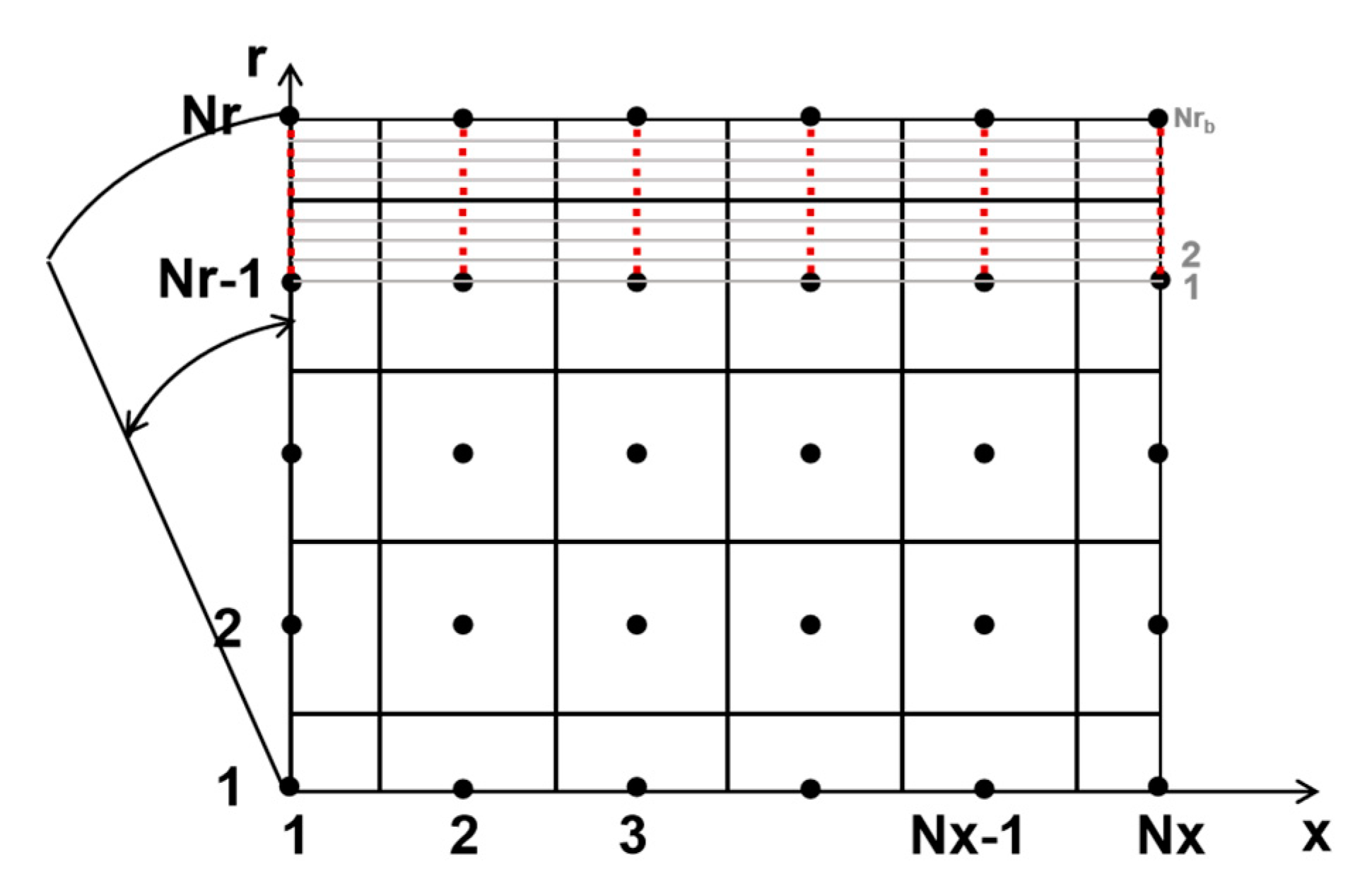
As the external node method is adopted in this paper, the grid division under the column coordinate system is shown in Figure 2. In the figure, the horizontal axis is the axial direction of the pipeline, containing a total of Nx nodes, and the vertical axis is the radial direction of the pipeline, containing a total of Nr nodes. When the boundary layer mesh is encrypted, the mesh between the Nr − 1 and Nr layers is encrypted, and the outermost encrypted mesh contains Nrb nodes.
In the discrete format of the calculation area, the calculation formula of the average oil concentration at the pipe section is as follows
c ¯ = 1 N r V i c i 1 N r V i
where c ¯ represents the average oil concentration at a certain axial node of the pipeline cross-section; c i represents the oil concentration value at the i-th radial node on the section; V i represents the control volume and circumferential direction at the corresponding node c i .

3.2. Governing Equation Discretization

3.2.1. Convection Equation Discretization

The form of the pure convection equation is as follows. Based on the basic form of the pure convection equation, the characteristic line method is used to solve the pure convection equation.
1 2 c t + u m c x = 0
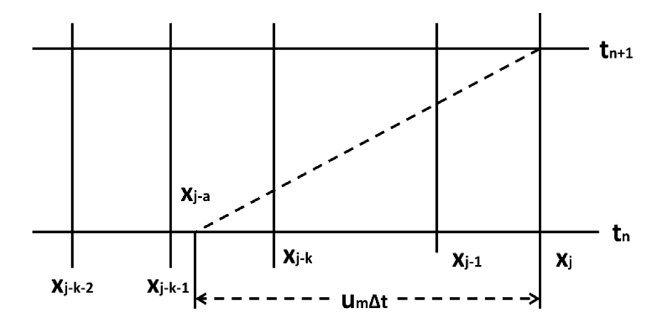
The above equations are discretized along the direction of characteristic lines. Figure 3 shows the principle of characteristics method. The slanted dotted line in the figure represents the direction of the characteristic line. The n-time layer is related to the concentration value on the (n + 1)-time layer, tn represents the n-time layer, tn+1 represents the (n + 1)-time layer, and x represents the axial coordinates of the pipeline. j, k is an integer, a is a real number, and Δ t represents the time interval between the n-time layer and the (n + 1)-time layer.
When only convection terms are considered, along the direction of the characteristic line
c j n + 1 = c j a n
Then, to calculate the concentration value of node j at (n + 1)-time layer, it is only necessary to calculate the concentration value at point j-a at n-time layer. Because a is a real number greater than zero, j-a may not fall on the divided grid nodes. Here, the concentration value at the j-k point of the grid node is used to approximate the concentration value at the j-a node. Suppose the relationship between the concentration distribution and the distance at n-time layer is as follows
x j k x j k a x j k x j k 1 = c j k c j k a c j k c j k 1
then
c j n + 1 = c j k n p ( c j k n c j k 1 n )
where
p = x j k + u m Δ t x j Δ x
Through the above formula, the concentration value of node j at (n + 1)-time layer can be obtained, and so on. The concentration value at each node, except the beginning of the pipeline (boundary condition) at (n + 1)-time layer, can be calculated.
The solution of the two-dimensional convection term is the same as the one-dimensional principle, except that the velocity in the two-dimensional pure convection equation is no longer the average velocity of the pipe cross section, but the specific velocity at a certain point of the pipe cross-section. In the calculation, the velocity can be considered in different regions.
In order to reduce the numerical diffusion effect of Equation (32), Casulli adopts one upwind point and two downwind points to carry out quadratic difference, and its calculation formula is as follows
c j n + 1 = c j k n 1 2 p ( c j k n c j k 1 n ) + 1 2 p 2 ( c j k + 1 n 2 c j k n + c j k 1 n )
When k = 0, the above formula is transformed into Lax–Wendroff format
c j n + 1 = c j k n p ( c j k n c j k 1 n ) 1 2 p ( 1 p ) ( c j k n 2 c j k 1 n + c j k 2 n )
Equation (34) does not introduce numerical diffusion effect, but there is a dispersion phenomenon. Equations (33) and (34) are weighted and averaged to obtain Equation (35), which is effective in most cases.
c j n + 1 = c j k n θ p 2 ( c j k + 1 n c j k 1 n ) p ( 1 θ ) ( c j k n c j k 1 n )   + θ p 2 ( c j k + 1 n 2 c j k n + c j k 1 n ) ( 1 θ ) p ( 1 p ) 1 2 ( c j k n 2 c j k 1 n + c j k 2 n )

3.2.2. Diffusion Equation Discretization

The pure diffusion equation form of the one-dimensional mixed oil model is as follows
1 2 c t = K 2 c x 2
Compared with the explicit format, the implicit format solution has the advantage of absolute stability. The following describes the method of implicitly solving the diffusion term. The format of implicit discretization is as follows
1 2 c i n + 1 c i n Δ t = K c i 1 n + 1 2 c i n + 1 + c i + 1 n + 1 ( Δ x ) 2
The recursive formula after organizing is as follows
c i n = 2 K Δ t ( Δ x ) 2 c i 1 n + 1 + ( 1 + 4 K Δ t ( Δ x ) 2 ) c i n + 1 2 K Δ t ( Δ x ) 2 c i + 1 n + 1
From the above formula, the relationship between the concentration of a certain point at the n-time layer and the concentration of three points at the (n + 1)-time layer can be obtained. The concentration value marked n above represents the concentration value of the known time layer, while the concentration value at (n + 1)-time layer has yet to be solved.
When n = 1 and i = 2, the above equation becomes
c 2 1 = 2 K Δ t ( Δ x ) 2 c 1 2 + ( 1 + 4 K Δ t ( Δ x ) 2 ) c 2 2 2 K Δ t ( Δ x ) 2 c 3 2
where c 1 2 is the boundary condition at the beginning of the pipeline, which is a known value. Move this term to the column vector at the right end of the equation, and use the same method to process the points at the end of the pipeline to obtain the following matrix. When the number of axial nodes in the pipeline is Nx, the tridiagonal matrix on the left is ( N x 2 ) × ( N x 2 )
[ 1 + 4 K Δ t ( Δ x ) 2 2 K Δ t ( Δ x ) 2 2 K Δ t ( Δ x ) 2 1 + 4 K Δ t ( Δ x ) 2 2 K Δ t ( Δ x ) 2 2 K Δ t ( Δ x ) 2 1 + 4 K Δ t ( Δ x ) 2 2 K Δ t ( Δ x ) 2 2 K Δ t ( Δ x ) 2 1 + 4 K Δ t ( Δ x ) 2 ] [ c 2 n + 1 c 3 n + 1 c 4 n + 1 c i 2 n + 1 c i 1 n + 1 ] = [ c 2 n + 2 K Δ t ( Δ x ) 2 c 1 n + 1 c 3 n c i 2 n c i 1 n + 2 K Δ t ( Δ x ) 2 c i n + 1 ]
where, c i n + 1 is approximated by c i n + 1 = c i 1 n + 1 according to the boundary conditions at the end of the pipeline. Then, the matrix becomes the following form; pay attention to the change in the coefficient in the lower right corner of the tridiagonal matrix and the change in the last term of the column vector on the right side of the equation
[ 1 + 4 K Δ t ( Δ x ) 2 2 K Δ t ( Δ x ) 2 2 K Δ t ( Δ x ) 2 1 + 4 K Δ t ( Δ x ) 2 2 K Δ t ( Δ x ) 2 2 K Δ t ( Δ x ) 2 1 + 4 K Δ t ( Δ x ) 2 2 K Δ t ( Δ x ) 2 2 K Δ t ( Δ x ) 2 1 + 2 K Δ t ( Δ x ) 2 ] [ c 2 n + 1 c 3 n + 1 c 4 n + 1 c i 2 n + 1 c i 1 n + 1 ] = [ c 2 n + 2 K Δ t ( Δ x ) 2 c 1 n + 1 c 3 n c i 2 n c i 1 n ]
With the help of the above tridiagonal matrix, the concentration value of each node at the next time layer can be solved according to the known concentration value of each node at the previous time layer.
The solution method of the two-dimensional diffusion term is similar to that of the one-dimensional one, which uses the form of diagonal matrix to relate the concentration value at the previous time layer with that of the next time layer to obtain a series of closed equations, and solve the whole equation at the same time step. Because the two-dimensional diffusion term includes both axial and radial directions, the diagonal matrix is more difficult to solve than the one-dimensional case. Since the solution is a global solution at the whole-time layer, all the internal nodes corresponding to the axial and radial directions at the whole-time layer need to be transformed into a column vector, so that the global solution can be performed at a time layer.
Due to the complexity of the penta-diagonal matrix, the penta-diagonal matrix is divided into two matrices with the same size, and the penta-diagonal matrix is the sum of the two matrices, namely Q = Q 1 + Q 2 . Now, Q 1 and Q 2 are described, respectively.
Firstly, the elements to be used in the matrix are defined
m = 2 D Δ t ( Δ r ) 2
n = 2 D Δ t ( Δ x ) 2
k = 1 + 4 D Δ t ( Δ x ) 2 + 4 D Δ t ( Δ r ) 2
In the expressions of the above three elements m, n and k, D is the diffusion coefficient. The diffusion coefficient of the model used in this paper is related to the position of the node in the pipeline, so the value of D at different nodes is different, which is uniformly represented by D here.
The matrix Q 1 is composed of smaller matrices A and B. The expression for Q 1 is as follows, where the value of unlisted elements is zero, the same as below
Q 1 = [ A B B A ] ( N x 2 ) ( N r 2 ) × ( N x 2 ) ( N r 2 )
where A and B are matrix composed of m, n, and k.
A = [ k + m n n k + m n n k + m + n ] ( N x 2 ) × ( N x 2 )
B = [ k n n k n n k + n ] ( N x 2 ) × ( N x 2 )
In the matrix Q 2 , the values of elements on two lines parallel to the main diagonal are not equal to zero, the values of the elements on the two lines are the same, and the two lines are symmetric regarding the main diagonal of Q 1 . The distance between the non-zero element m in the first row and the first element in the first row is N x 2 to determine the position of the two lines.
Q 2 = [ m m m m ] ( N x 2 ) ( N r 2 ) × ( N x 2 ) ( N r 2 )
The matrix P on the right side of the equation represents the known concentration value corresponding to each node at the time layer. The matrix on the right side of the equation (denoted as P here) has the following form
P = P 1 + P 2
P1 and P2 can be expressed by column vectors, respectively, as
P 1 = [ c 2 , 2 n c 2 , 3 n c 2 , N x 1 n c 3 , 2 n c 3 , 3 n c 3 , N x 1 n c N r 1 , 2 n c N r 1 , 3 n c N r 1 , N x 1 n ] 1 × ( N r 2 ) ( N x 2 ) T
P 2 = [ b c 2 , 1 n 0 0 b c 2 , 1 n 0 0 b c N r 1 , 1 n 0 0 ] 1 × ( N r 2 ) ( N x 2 ) T
where, c i , j represents the oil concentration value of the rear oil corresponding to the radial node i and the axial node j.
The matrix M to be solved represents the concentration value of each node at the new time layer, and its expression is as follows
M = [ c 2 , 2 n + 1 c 2 , 2 n + 1 c 2 , N x 1 n + 1 c 3 , 2 n + 1 c 3 , 3 n + 1 c 3 , N x 1 n + 1 c N r 1 , 2 n + 1 c N r 1 , 2 n + 1 c N r 1 , N x 1 n + 1 ] 1 × ( N r 2 ) ( N x 2 ) T
Then, the whole system is expressed in the form of matrix product as
Q × M = P

3.2.3. Boundary Condition Dispersion

At the pipe axis and the pipe wall
t 0 : c r | r = 0 = c r | r = R = 0
The discretized format is
t 0 : c 2 = c 1 , c N r = c N r 1
where c represents oil concentration, %; x represents the axial position of the calculated pipe segment, m.

3.2.4. Proposal and Calculation Method of Deviation Volume

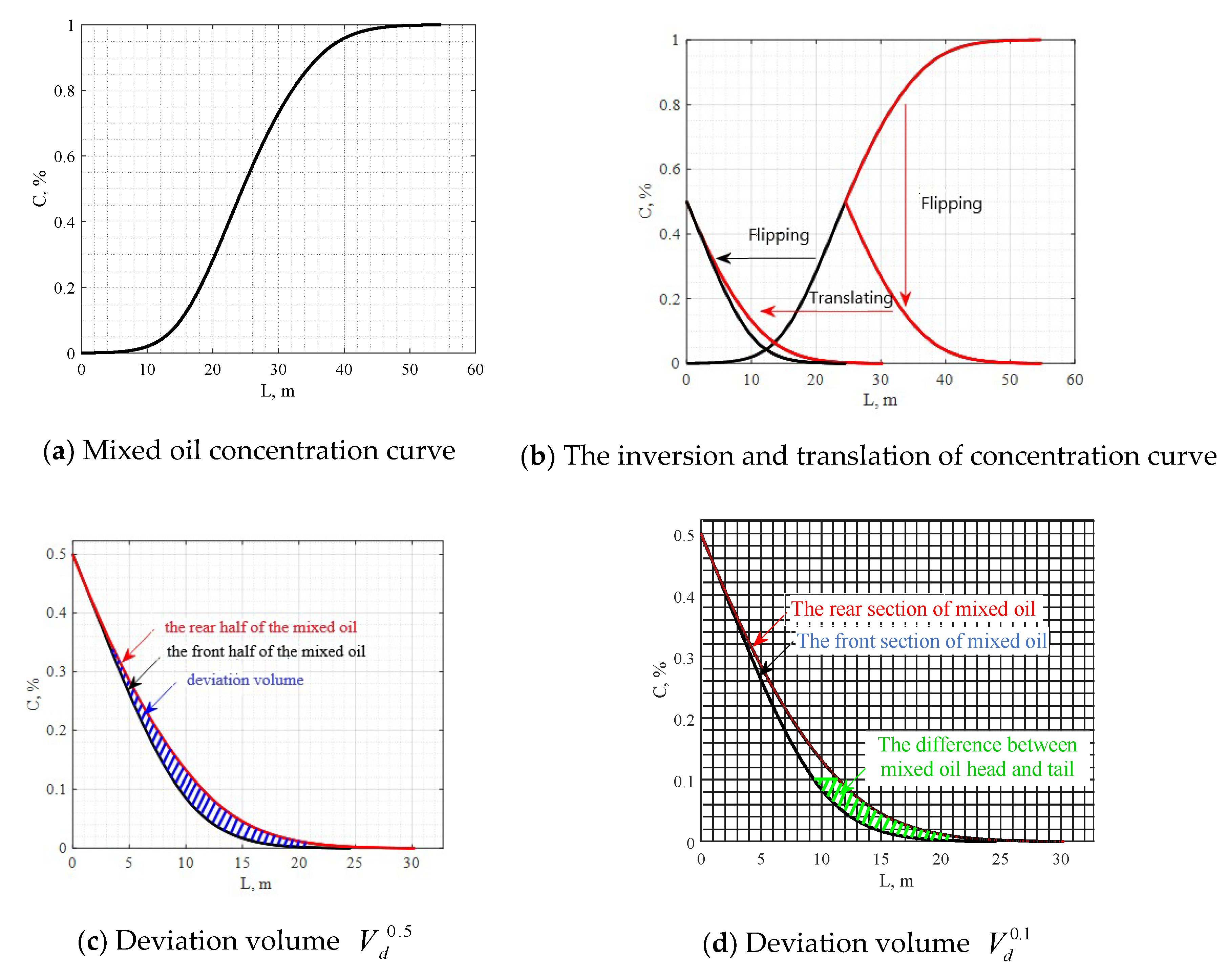
At present, there is no complete method to measure the overall asymmetry of the mixed oil concentration curve. In this paper, the concept of deviation volume is proposed to characterize the degree of asymmetry in the concentration curve of mixed oil. Figure 4a shows the curve of mixed oil concentration; the horizontal axis is the length of mixed oil. The vertical axis is the concentration of the rear oil. The interface of the mixed oil section is asymmetric with respect to the 50% concentration. To measure the degree of asymmetry of the mixed oil concentration curve, the curve is divided into two parts: the front part and the back part. The front part, i.e., the part where the mixed oil head is located, is the left part of the curve, where the oil concentration before it is greater than or equal to 50%. The back part, i.e., the part where the mixed oil tail is located, is the right half of the curve, where the oil concentration of rear oil is greater than 50%.
The volume of the rear oil products contained in the first half of the mixed oil section is
V f 0.5 = L f π R 2 c i d l
Vf represents the volume of the rear oil contained in the first half of the mixed oil; the lower index f represents the front-part of the mixed oil; the upper index 0.5 represents that the concentration of the front oil is greater than or equal to 0.5; R represents the radius of the pipeline; Lf represents the length of the first half of the mixed oil; ci represents the concentration of the rear oil. Similarly, the volume of the front oil contained in the second half of the mixing oil section is
V t 0.5 = L t π R 2 ( 1 c i ) d l
Vt represents the volume of the front oil contained in the second half of the mixed oil; the lower index t represents the tail-part of the mixed oil; the upper index 0.5 represents that the concentration of the rear oil is greater than 0.5; R represents the radius of pipeline; Lt represents the length of the second half of the mixed oil.
Flip the first half of the oil mixture concentration curve, flip and translate the second half, as shown in Figure 4b. The two halves are similar in shape but do not overlap. The area of the gap formed between the two curves is used to represent the degree of asymmetry of the two oil-mixed curves, as shown in the shaded part of Blue in Figure 4c. The area is the same as the length unit, and the unit is the volume after multiplying by the pipe section area. The area of the blue shaded part in Figure 4c is defined as the deviation volume. Its physical meaning is the difference between the volume of the front oil in the second half of mixing oil and the volume of the rear oil in the first half of mixing oil. The calculation method is
V d 0.5 = V t 0.5 V f 0.5
where Vd represents the deviation volume, Vf represents the volume of the rear oil in the first half of the mixed oil, and Vt represents the volume of the front oil in the first half of the mixed oil. The deviation volume can reflect the asymmetry of the entire mixed oil concentration curve, and has a clear physical meaning.
When analyzing the difference between the mixing oil head and the mixing oil tail, the volume of the rear oil contained in the mixing oil head is
V f 0.1 = L f 0.1 π R 2 c i d l
The volume of the front oil contained in the mixing oil tail is
V t 0.1 = L t 0.1 π R 2 ( 1 c i ) d l
Then, the difference between mixed oil head tail can be described by
V d 0.1 = V t 0.1 V f 0.1
The upper index 0.1 indicates that the comparison is the volume difference between the front oil contained in the mixed oil tail and the rear oil contained in the mixed oil head. From the graph of the concentration curve, it represents the deviation volume corresponding to the green part in Figure 4d.
The dimensionless deviation volume is used in this paper. The characteristic length of the pipe is the pipe diameter D, and the dimensionless deviation volume is defined as
V d * = V t * V f *
The calculation method is
V d * = V d D 3
The absolute value of the deviation volume indicates the degree of asymmetry of the concentration curve. When the deviation volume value is positive, it means that the second half of the mixed oil contains more front oil than the rear oil contained by the first half. When the deviation volume is negative, it means that the second half of the mixed oil contains less front oil than the rear oil contained by the first section.

4. Results and Discussion

4.1. Basic Data

The relative parameters of oil density and viscosity used in the calculation process are shown in Table 1 and Table 2.

4.2. Model Validation

To validate the above models, we test the grid independence of numerical results, and compare the numerical results with physical experiments and famous empirical formulas as follows.

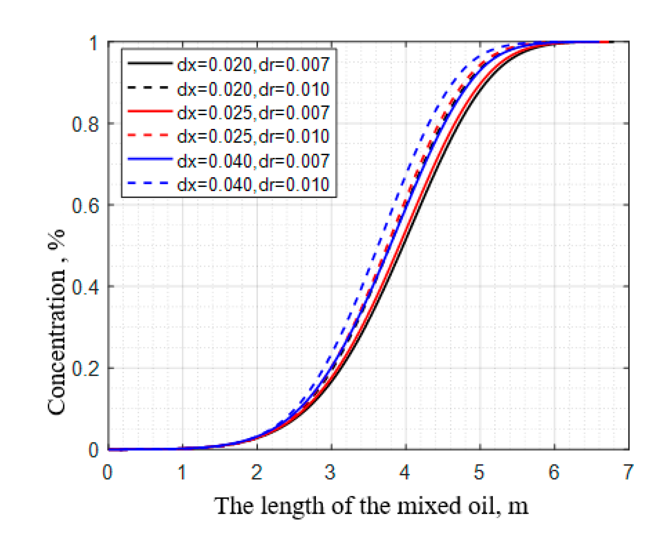
4.2.1. Grid Independence Test

The grid independence test of the model is shown in Figure 5. Theoretically, the calculation results are more accurate using a denser mesh, but too dense a mesh may lead to a too-long computational time and insufficient computer memory. As shown in Figure 5, when dx and dr continue to decrease, the mixed oil concentration curve of the products pipeline changes little, and the length of the mixed oil section of the products pipeline changes very slightly. To improve the calculation efficiency, this paper finally selects the model grid parameters dx = 0.025 m, dr = 0.007 m for simulation.

4.2.2. Experimental Verification

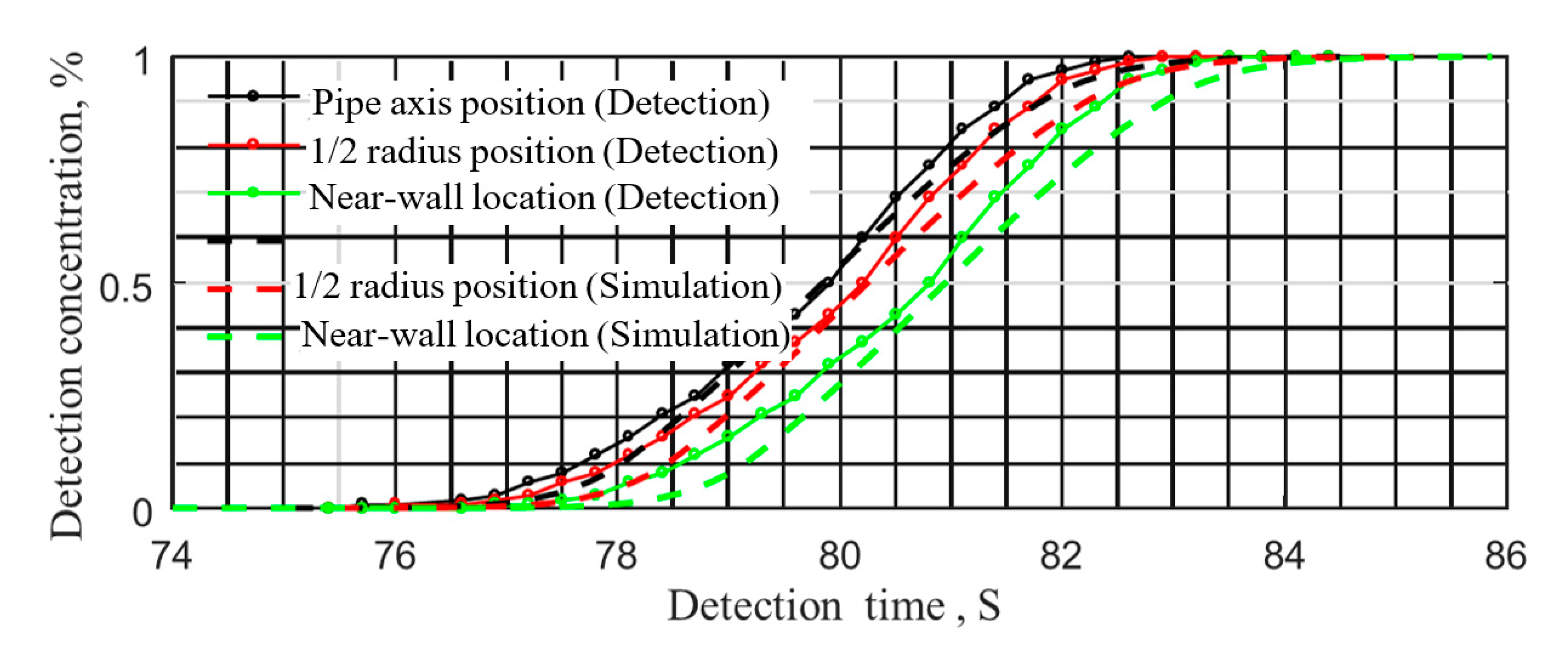
The simulation results of the two-dimensional model were compared with the loop data obtained by the research team. A water–sodium chloride aqueous solution was used as the experimental medium. The length of the experimental pipe is 200 m. The length of the numerical simulation pipe is 200 m, and the simulation medium and pipe parameters are the same as the experiment. The length of the mixed liquid measured in the experiment is 9.2 m. The numerically calculated length of the mixed liquid is 9.5 m. Their deviation is as low as 3.3%. The three solid dotted lines in Figure 6 represent the concentrations detected by the probes at different radial positions of the experimental loop. The dotted line represents the numerical simulation result. The comparison shows that the numerical simulation and experimental results are basically consistent.

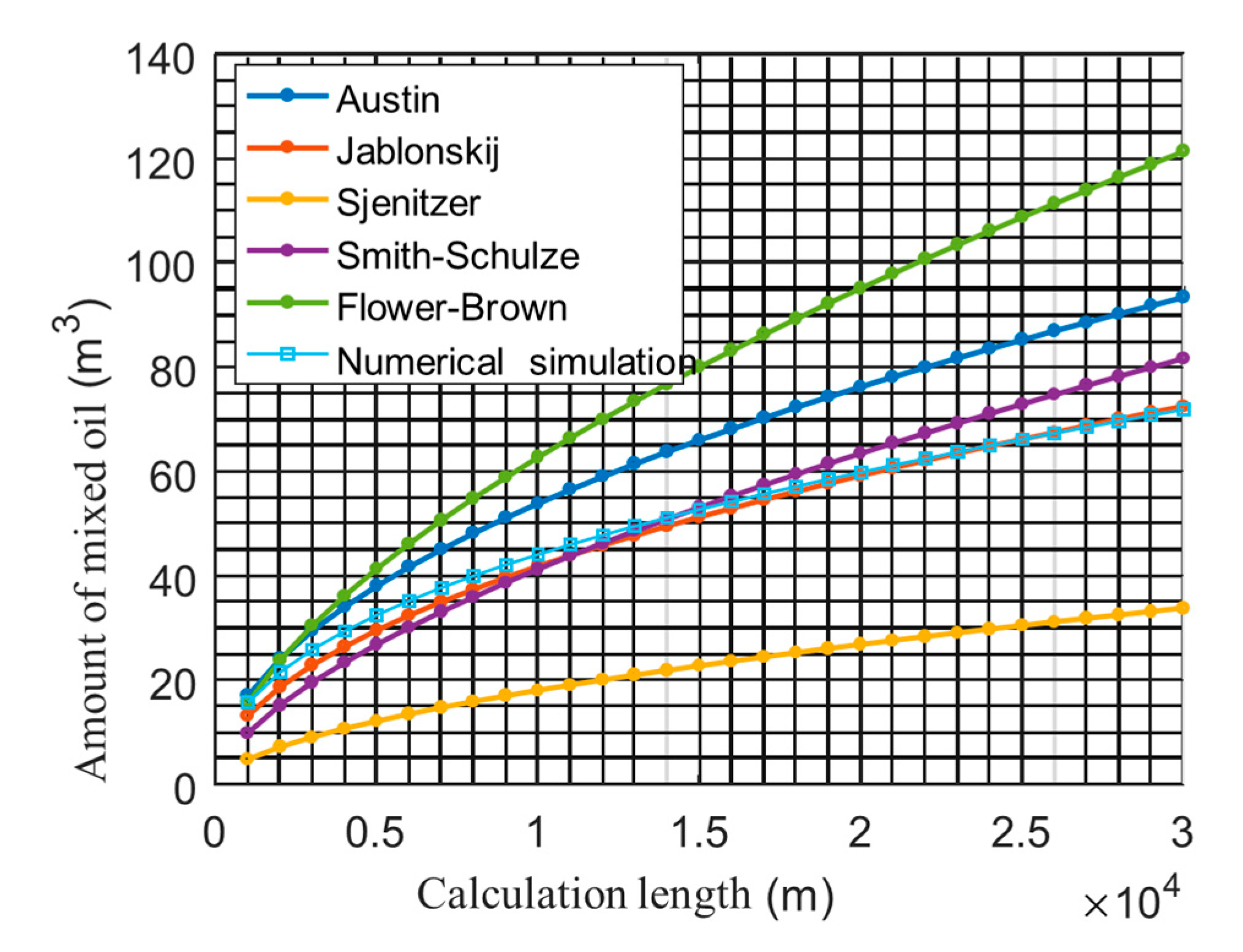
4.2.3. Empirical Formula Verification

Figure 7 shows the comparison result of the mixed oil quantity obtained by the numerical simulation and the empirical formula. The total length of the simulated pipeline is 30 km, and the simulated transportation temperature is 20 °C, regardless of temperature changes along the pipeline. The order of oil delivery is 0# diesel first and 90# gasoline later. The pipeline flow rate is 1 × 10³ m3/h. The numerical simulation results are the closest to Jablonskij’s empirical formula [23].

4.3. Analysis of Concentration Field Distribution Characteristics

4.3.1. Comparison of One-Dimensional Model and Two-Dimensional Model

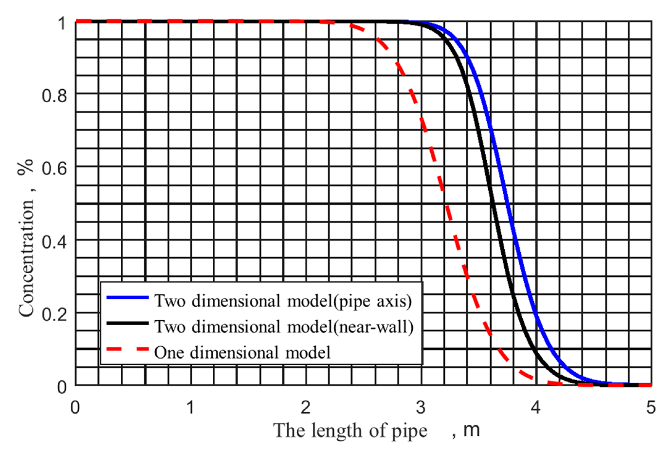
The solution results of the one-dimensional model and the two-dimensional model are shown in Figure 8. The red dashed line in the figure is the calculation result of the one-dimensional model. After testing, the deviation volume is 0, which is a center-symmetric figure. The blue and black solid lines, respectively, indicate the changes in the concentration of oil at the axis of the pipeline and the pipe wall when the two-dimensional model is used. Through observation, it can be found that the mixed oil concentration curve calculated by the two-dimensional model is asymmetric. This asymmetry is caused by uneven flow velocity across the pipe section. The calculation results of the one-dimensional model and the two-dimensional model are different in the length of the mixing section, the position of the mixed oil section, and the degree of symmetry of the mixed oil concentration curve. This is due to the large model error of the one-dimensional model itself, which can only describe the change in the mixed oil concentration in the axial direction of the pipeline. In the calculation process, the average concentration used in the one-dimensional model is only related to the axial position, and the concentration, average density and average viscosity are considered unchanged on the same section of the pipeline. The two-dimensional model continuously updates the average density and average viscosity at each node by calculating the concentration of each node.
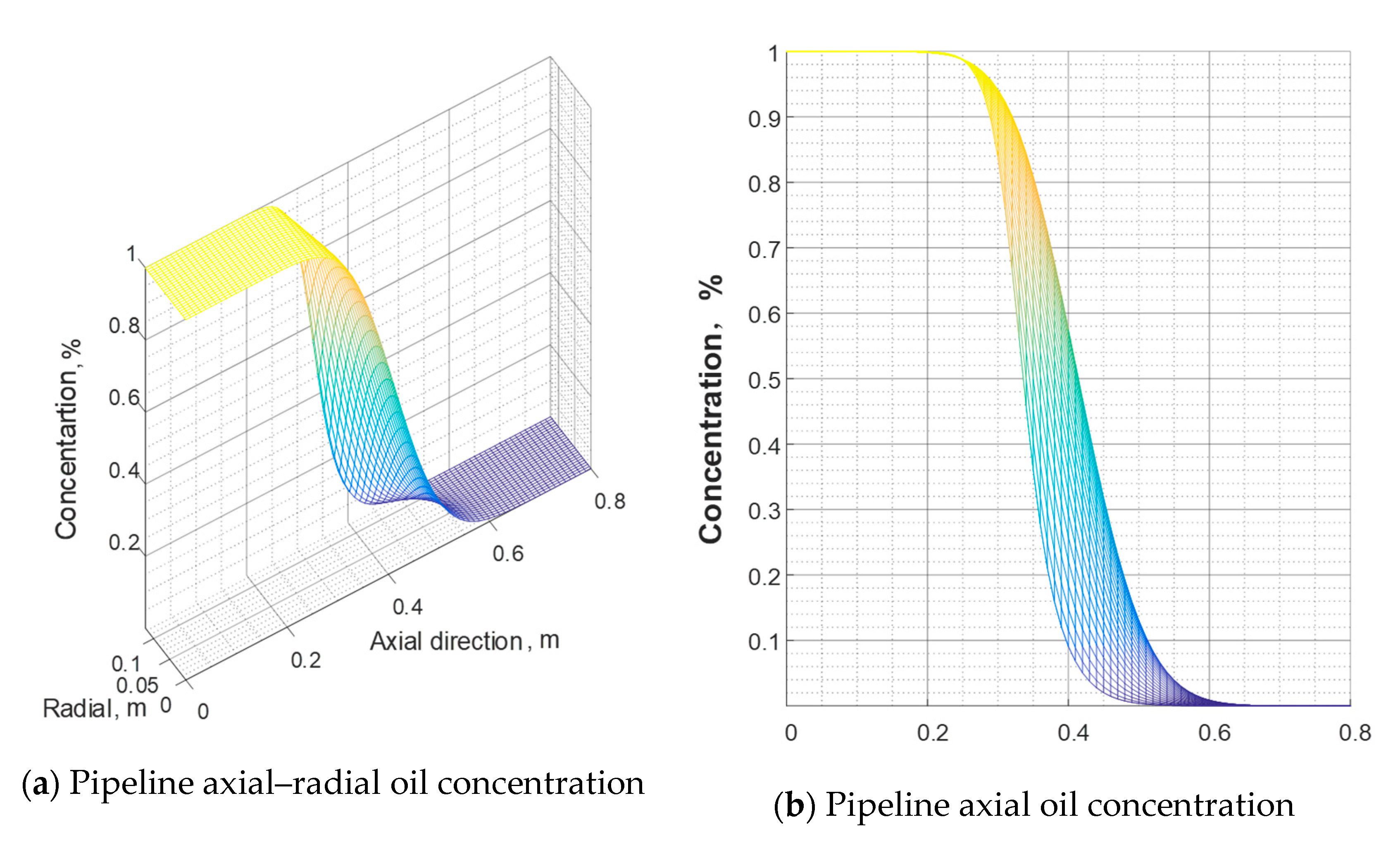
Figure 9 shows the numerical simulation results of the two-dimensional model. At the axis of the pipeline, the replacement speed of oil is faster than that at the pipe wall, because the flow rate of the oil at the center of the pipeline is greater than that at the wall.

4.3.2. Comparison of the Effects of Convection and Diffusion on the Mass Transfer Process

In this paper, the time-division method is used to solve the convection–diffusion equation. The convection–diffusion equation is divided into a convection equation and diffusion equation to be solved separately. One of the advantages of this is that it can solve the convection equation and the diffusion equation separately, and compare the influence of the two through the numerical simulation results, and observe the concentration of oil when only the convection equation or only the diffusion equation is calculated. However, in the actual oil-mixing process, convection and diffusion always exist simultaneously. This paper compares the solution results of pure convection equation and pure diffusion equation, aiming to compare the strength of the effect of convection on diffusion, and deepen the intuitive understanding of the effects of convection and diffusion.
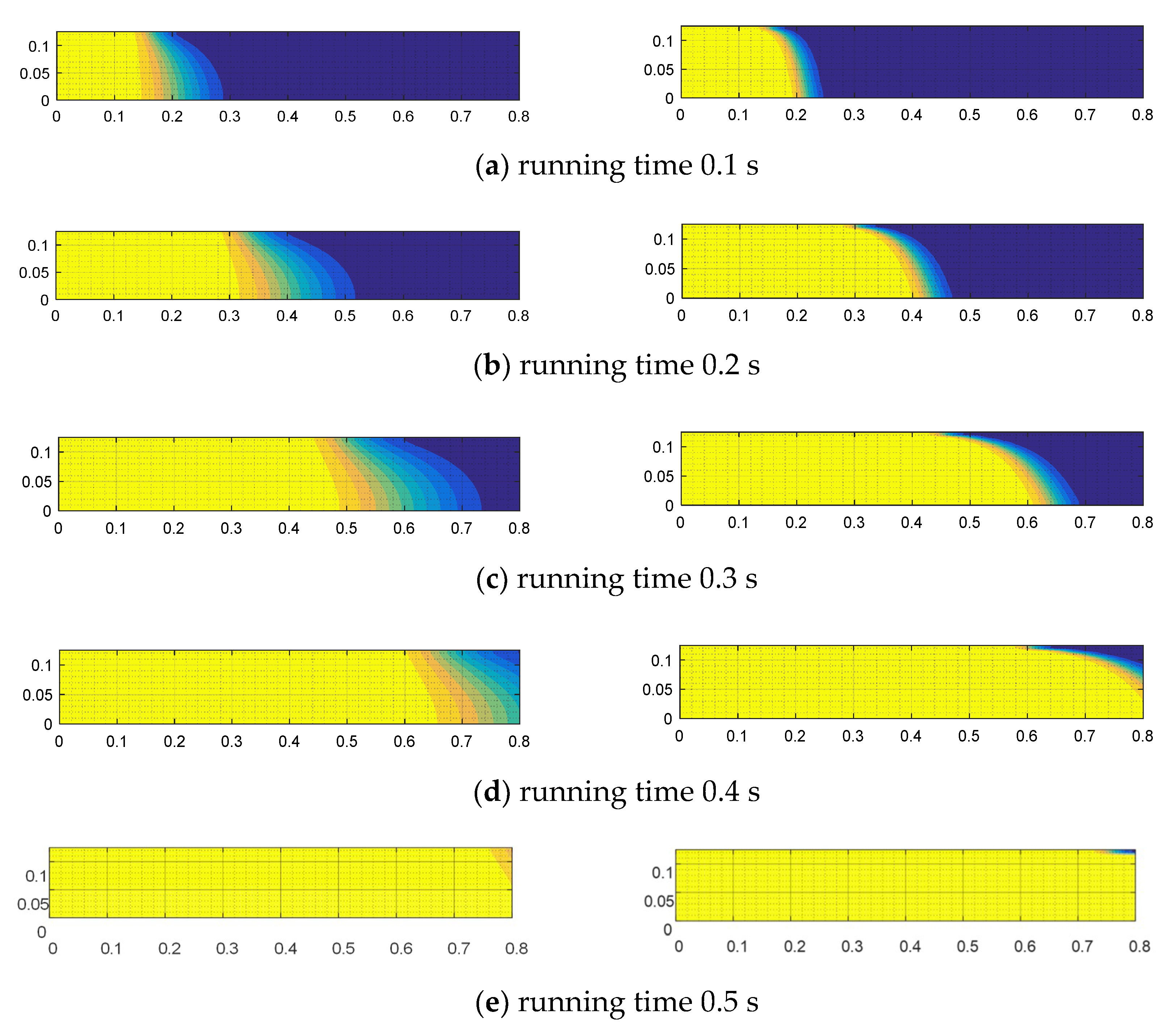
The left side of Figure 10 shows the simulation results of simultaneous calculation of mixed oil concentration and diffusion, and the right column shows the distribution of oil mixture concentration when only convection terms are calculated. The abscissa in the figure represents the axial direction of the pipeline, and the ordinate represents the radial direction of the pipeline. The length of the pipe used for calculation is 0.8 m and the pipe diameter is 250 mm. The simulated conveying temperature is 20 °C. Run 0# diesel first, then 90# gasoline. The average flow velocity is 1.8 m/s. Figure 10a–e shows the oil concentration distribution in the calculated pipe section corresponding to the running time of 0.1 s, 0.2 s, 0.3 s, 0.4 s and 0.5 s.
In the initial stage of oil mixing, the oil mixing speed is faster. After the occurrence of the mixed oil section, the mixed oil section acts as an isolation for the two product oils, and the growth rate of the mixed oil amount slows down. At this flow rate, when the running time is 0.5 s, the mixed oil section has basically left the calculation pipe section. When only convection is calculated, the product oil concentration distribution is basically consistent with the flow velocity distribution at the pipe interface, which is not much different from the product oil concentration distribution when the convection diffusion equation is solved.
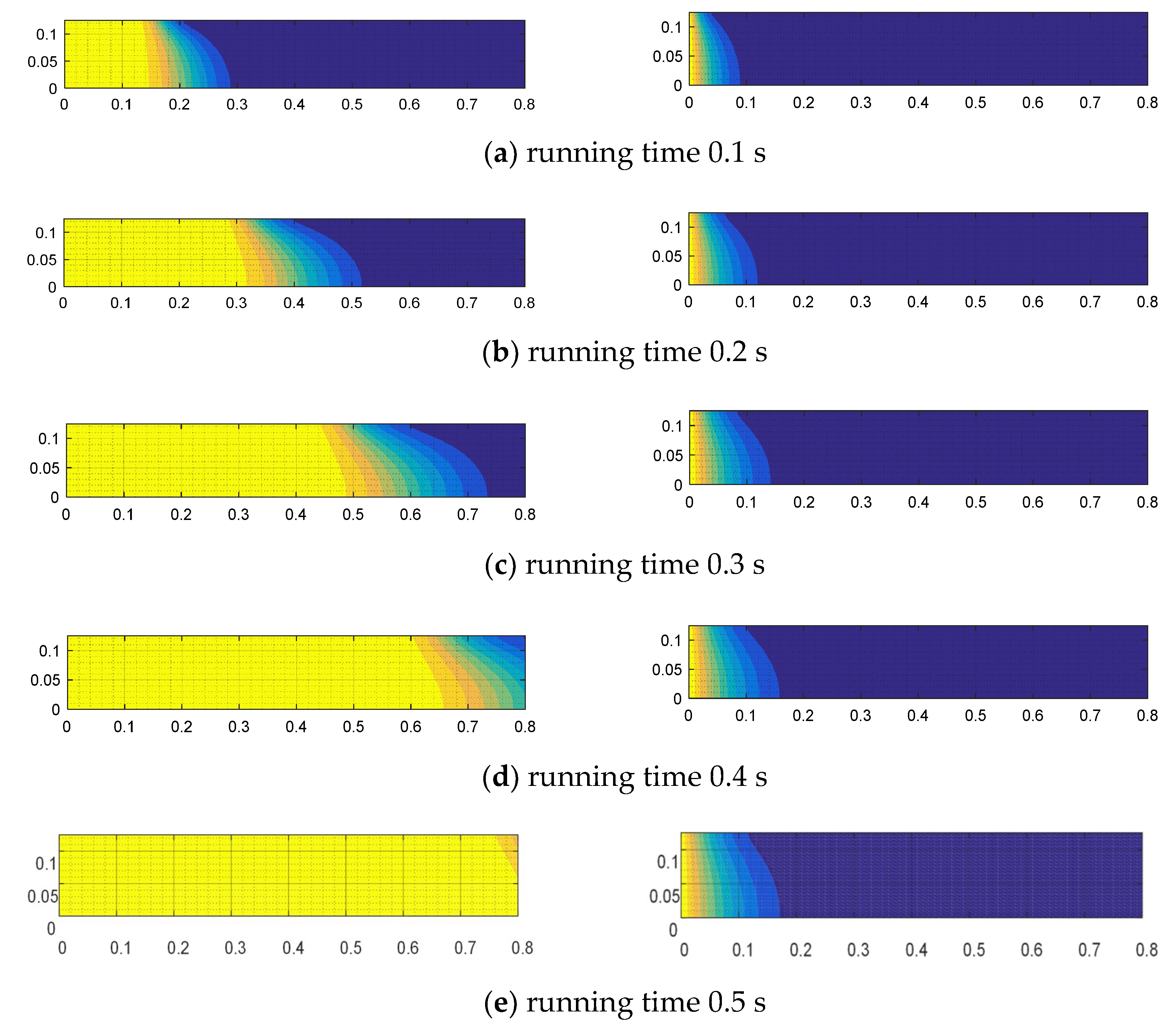
Figure 11 shows the comparison of the oil concentration distribution between the two-dimensional model and only the diffusion term. The left side is the calculation result when the convection term and the diffusion term are calculated at the same time, and the right side is the result when only the diffusion term is calculated. Figure 11a–e corresponds to running times of 0.1 s, 0.2 s, 0.3 s, 0.4 s and 0.5 s, respectively. The speed of diffusion is obviously slower than that of convection. When calculating the diffusion coefficient, the distance between the calculation position and the pipe wall is also considered, and different formulas are used for calculation in different areas. At the bottom layer of laminar flow, the diffusion coefficient is equal to the molecular diffusion coefficient, and a constant is used in the calculation process. In the buffer layer and the turbulent core area, the size of the turbulent diffusion coefficient is positively related to the distance from the pipe wall, so the concentration field under the action of diffusion also shows that the amount of oil mixed at the pipe axis is more than that at the pipe wall.
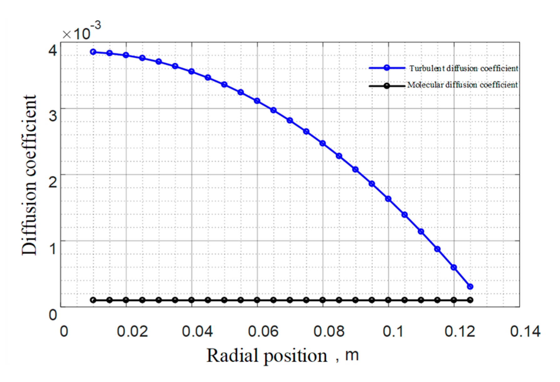
According to the formula, the diffusion coefficient in the model is only related to the radial position, and the diffusion coefficient at the same radial position is considered the same. Figure 12 shows the distribution of the calculated turbulent diffusion coefficient and molecular diffusion coefficient at different radial positions of the pipe section. In the calculation process, the molecular diffusion coefficient is a fixed value. It can be seen from the figure that the turbulent diffusion coefficient takes the largest value at the pipe axis and the smallest value at the pipe wall. This is also the reason why when only the diffusion term is calculated in Figure 11, the oil spreads faster at the axis of the pipe and slower at the pipe wall.

4.3.3. The Impact of the Viscous Sublayer

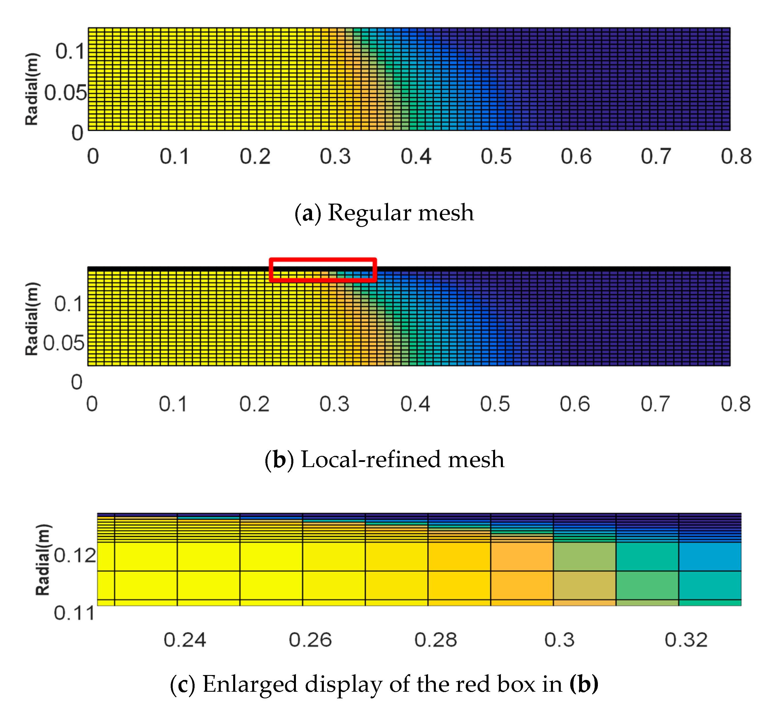
To measure the impact of the viscous sublayer on the asymmetry of mixed oil, and to describe the oil velocity distribution more accurately at the viscous sublayer, the boundary layer grid was dense, as shown in Figure 13. Among them, (a) is the calculation result when the boundary layer mesh is not dense, (b) is the effect of encrypting the original outermost grid, and (c) is the enlarged display of the red box in (b).
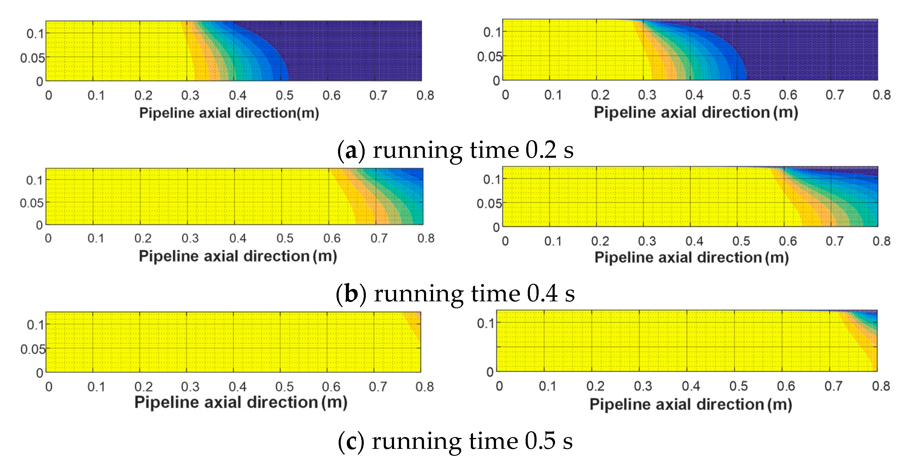
Figure 14 compares the distribution of oil concentration in the pipe section before and after the boundary layer mesh refinement. The left column is the simulation effect when the boundary layer mesh is not refined, and the right column is the refined effect. (a–c) correspond to a running time of 0.2 s, 0.4 s and 0.5 s respectively. Comparing the left and right columns of Figure 14a, in the initial stage of oil mixing, the oil concentration distribution after the boundary layer mesh refinement is roughly similar. Comparing the left and right columns of Figure 14b, as the calculation time increases, the effect of boundary layer mesh refinement gradually manifests. The refinement of the boundary layer mesh not only affects the oil concentration distribution close to the pipe wall, but also affects the oil concentration distribution at the center of the pipeline. Comparing the left and right columns of Figure 14c, after considering the refinement of the boundary layer mesh, the mixing of oil close to the pipe wall is significantly slower. In the right column of Figure 14c, close to the pipe wall, you can see the mixed oil tail trace left by the front oil.

4.4. Numerical Analysis of Influencing Factors of Asymmetry Distribution

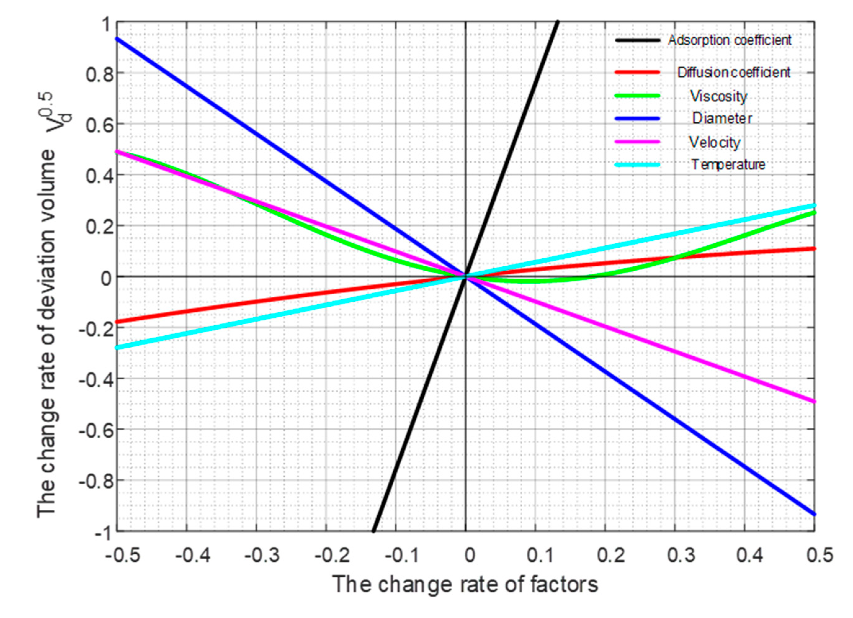
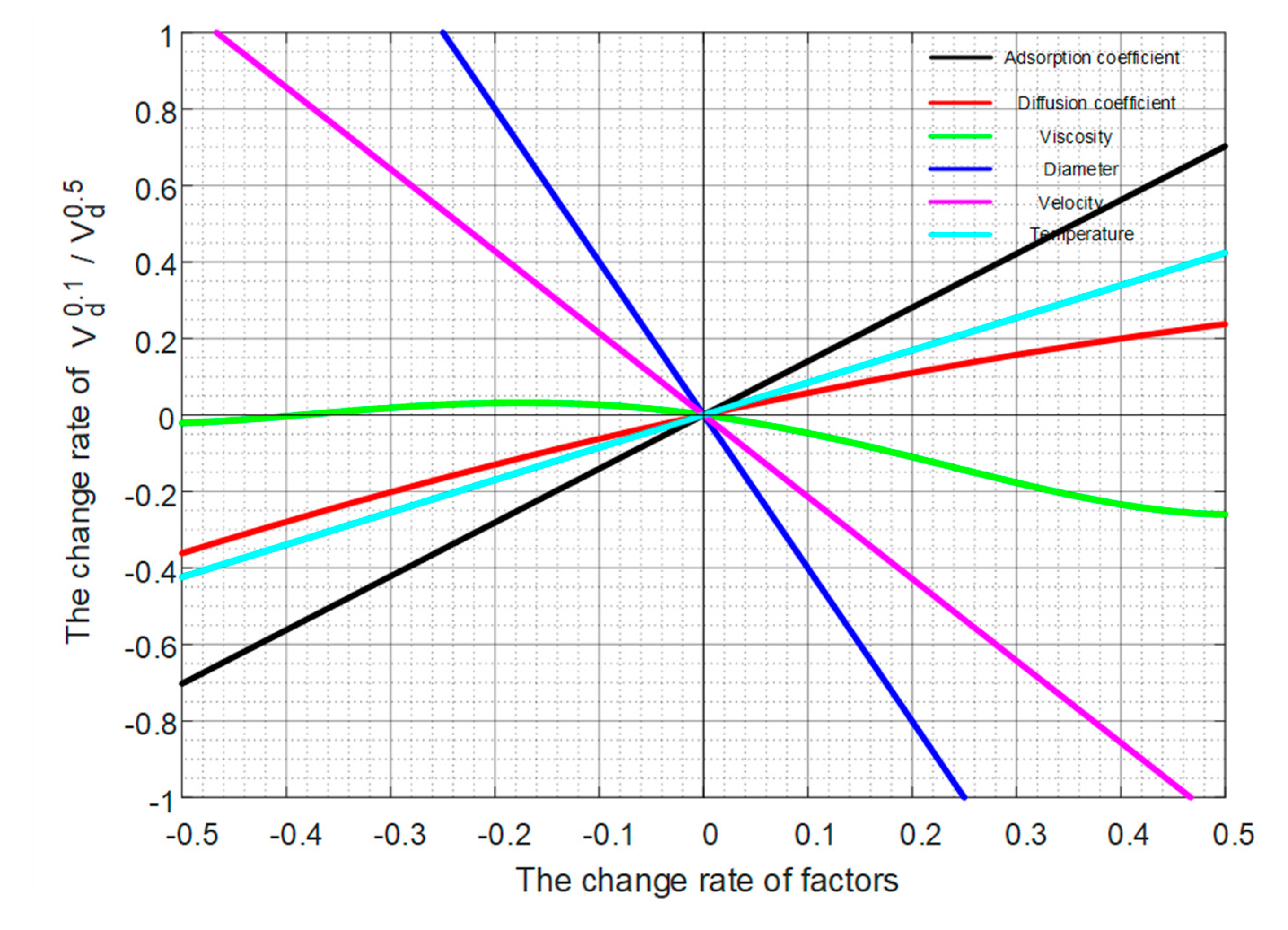
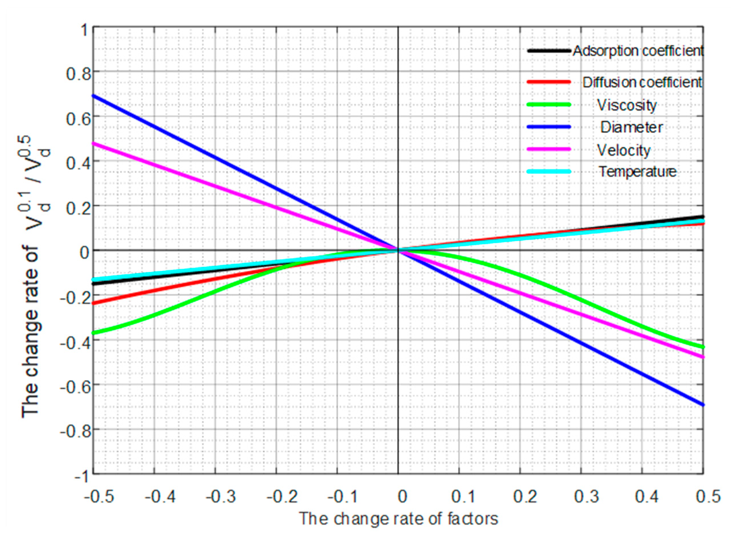
It can be seen from the analysis of the distribution characteristics of the concentration field that the concentration distribution on the pipeline interface is not uniform. To further investigate the effect of influencing factors on the asymmetry of the concentration curve, we analyze them one by one in this section. The factors are adsorption coefficient, viscosity, diffusion coefficient, temperature, pipe diameter, velocity. The details of the results and analyses can be found in the Supplementary Materials. Based on the detailed analyses, we further carried out a sensitivity analysis of these factors, as shown in the following four figures.
In Figure 15, when the changing rate of influencing factors is +10%, the changing rate of deviation volume Vd0.5 is: +75.8%, −18.7%, −9.8%, +5.6%, +2.7%. The degree of influence of each factor on the deviation volume Vd0.5, in descending order, is adsorption coefficient, pipe diameter, average flow velocity, temperature, and diffusion coefficient. Among them, the adsorption coefficient and the thermometer diffusion coefficient have a positive effect, while the pipe diameter and flow velocity have a negative effect. The oil viscosity has non-linear relationship with the deviation volume. When the viscosity is increased, the variation rate of the deviation volume first decreases slightly, and then increases.
The sensitivity analysis of the deviation volume Vd0.1 is shown in Figure 16. When the changing rate of the influencing factor is +10%, the changing rate of the offset volume Vd0.1 is: −40.0%, −21.4%, +14.1%, +8.5%, +5.7%. Thus, the degree of influence of each factor on the deviation volume Vd0.1 in descending order is pipe diameter, average flow velocity, adsorption coefficient, temperature, and diffusion coefficient. Among them, the adsorption coefficient and the thermometer diffusion coefficient have a positive effect, while the pipe diameter and flow velocity have a negative effect. The oil viscosity has no linear relationship with the offset volume Vd0.1 and its influence are small.
The sensitivity analysis of the ratio of the two deviation volumes (Vd0.1/Vd0.5) is shown in Figure 17. When the changing rate of the influencing factor is +10%, the rate of change in the ratio of the two deviation volumes is: −13.8%, −9.6%, +3.3%, +3.0%, +2.6%. The change in the influencing factor does not exceed 4% when the changing rate is +10%. The degree of influence of each factor on the ratio of the two in descending order is pipe diameter, average flow velocity, diffusion coefficient, adsorption coefficient, and temperature. Among them, the adsorption coefficient and the thermometer diffusion coefficient have a positive effect, while the pipe diameter and flow velocity have a negative effect. The oil viscosity has no linear relationship with the ratio of the two and its influence is small. The influence of various factors on the ratio of the two is like the influence on the deviation volume Vd0.1, but the influence of the contrast value is smaller.
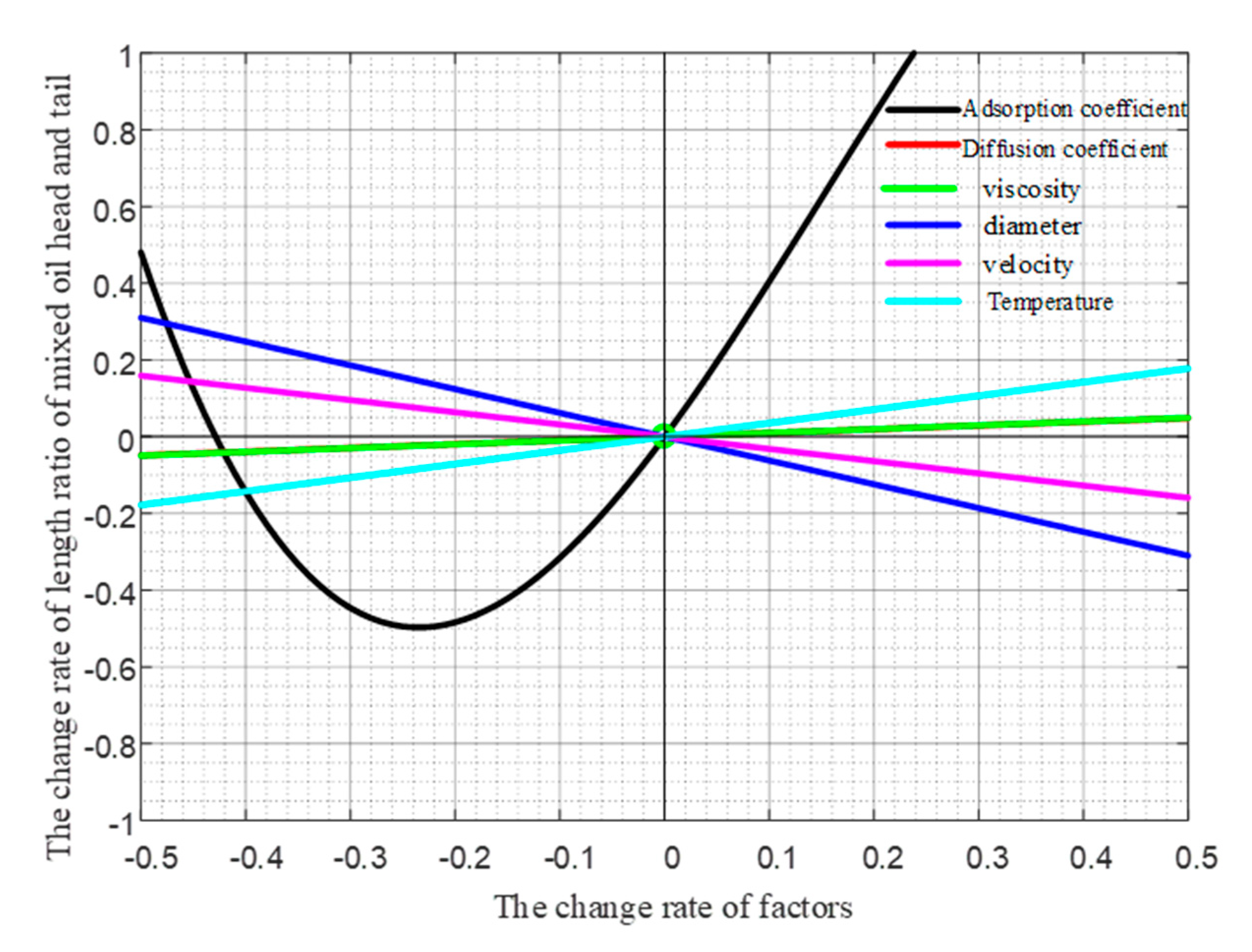
Figure 18 shows the sensitivity analysis of the sensitivity analysis of the ratio of mixed oil head to mixed oil tail length. When the changing rate of influencing factors is +10%, the changing rate of the ratio (mixed oil head/mixed oil tail length) is: +40.4%, −6.2%, +3.5%, −3.2%, +1.0%, +0.9%. The degree of influence of each factor on the ratio of the two, in descending order, is adsorption coefficient, pipe diameter, temperature, average flow rate, oil viscosity, diffusion coefficient. Among them, it is positively correlated with adsorption coefficient, temperature, oil viscosity and diffusion coefficient, and negatively correlated with pipe diameter and average flow velocity.

5. Conclusions

A mathematical model representing the asymmetry of mixed oil concentration, modified by polar adsorption near pipe wall, is established. The model is validated by experiments and empirical formula. Factors influencing the asymmetry are analyzed in detail. Based on this, a sensitivity analysis is made to quantify the influencing content of each factor. The concept of deviation volume is proposed for the first time to represent the asymmetry of mixed oil. It can be used to quantitatively define the asymmetry of mixed oil concentration curve. Thus, the study on mixed oil concentration is put forward from the qualitative phenomenon to the quantitative analysis. This study is the first report on the local characteristics of mixed oil concentration rather than previous studies to treat the development of mixed oil as a whole, so that more accurate mixed oil cutting in batch transportation of multi-product oils in pipeline engineering has a powerful tool.

Supplementary Materials

The following are available online at https://www.mdpi.com/1996-1073/13/23/6398/s1.

Author Contributions

Y.W. has contributed to the model derivation, numerical methods, data analysis, conclusion, and article revision; B.W. has contributed to the coding, simulation, and draft of the article; Y.L. (Yang Liu) has contributed to the article revision; Y.L. (Yongtu Liang) has contributed to the concept design and language polishing. All authors have read and agreed to the published version of the manuscript.

Funding

This research was funded by National Natural Science Foundation of China (NSFC), grant number No. 51576210 and No. 51874325. The APC was funded by NSFC No. 51576210. Baoying Wang was sponsored by the China Scholarship Council No. 201806440152. It was also supported by Science Foundation of China University of Petroleum, Beijing (No. 2462020YXZZ045).

Conflicts of Interest

The authors declare no conflict of interest.

References

  1. Liu, K.; Li, Y. Optimal treatment of mixed oil in product oil pipeline. Chem. Eng. Equip. 2019, 12, 112–114. [Google Scholar] [CrossRef]
  2. Shao, T. Study on scheduling optimization of batch sequential transportation of refined oil pipeline. Petrochem. Technol. 2018, 25, 235. [Google Scholar]
  3. Shadloo, M.S.; Rahmat, A.; Karimipour, A.; Wongwises, S. Estimation of pressure drop of two-phase fluid in horizontal pipes using artificial neural networks. J. Energy Resour. Technol. 2020, 142, 112110. [Google Scholar] [CrossRef]
  4. He, G.; Tang, D.; Wang, J.; Liang, Y. Prediction of mixed oil tailings based on gamma-chi-2 distribution. Oil Gas Storage Transp. 2019, 38, 58–65. [Google Scholar]
  5. Yang, X. Oil Pipeline Design and Management; China University of Petroleum Press: Dongying, China, 2006; pp. 270–286. [Google Scholar]
  6. Mostafaei, H.; Castro, P.M.; Relvas, S.; Harjunkoski, I. A holistic MILP model for scheduling and inventory management of a multiproduct oil distribution system. Omega-Int. J. Manag. Sci. 2019, 98, 102110. [Google Scholar] [CrossRef]
  7. Zhang, H.; Liang, Y.; Laio, Q.; Ma, J.; Yan, X. An MILP approach for detailed scheduling of oil depots along a multi-product pipeline. Pet. Sci. 2017, 14, 434–458. [Google Scholar] [CrossRef] [Green Version]
  8. Yu, T.; Yu, Y.; Wei, L. Interface detection of refined oil pipeline and control of oil mixture. Nat. Gas Pet. 2013, 5, 5–8. [Google Scholar]
  9. Guo, Y. A new method to improve the tracking accuracy of mixed oil interface of product oil pipeline. Oil Gas Storage Transp. 2010, 29, 908–909. [Google Scholar]
  10. Lu, J. Eigenline method and differential method for convection-dominant diffusion problems. Comput. Phys. 1989, 4, 486–494. [Google Scholar]
  11. Deng, S.; Pu, J. Comparison of two-dimensional and one-dimensional mixed oil models for sequential transportation of refined oil products. Oil Gas Storage Transp. 1997, 1, 16–18. [Google Scholar]
  12. Zheng, J.; Jiang, M. Optimization solution of two-dimensional model for sequential delivery of product oil pipeline. Mech. Pract. 2014, 36, 574–579. [Google Scholar]
  13. Ma, G.; Bai, R. Theoretical numerical Analysis of two-dimensional Oil Mixture in Product Oil Pipeline. Oil Gas Field Ground Eng. 2018, 37, 47–52. [Google Scholar]
  14. Wang, J. Oil mixing problem in sequential Transmission of Shicai Pipeline. Oil Gas Field Ground Eng. 2017, 36, 41–44, 52. [Google Scholar]
  15. Zhao, H. Study on Sequential Conveying Characteristics of Refined Oil Pipeline. Master’s Thesis, China University of Petroleum (East China), Dongying, China, 2008. [Google Scholar]
  16. Zhang, Q.; Wang, H.; Lu, Y. Concentration of mixed oil in phoenics numerical simulation pipeline. Nat. Gas Pet. 2007, 3, 28–31. [Google Scholar]
  17. Wang, Z.; Wang, Y. Numerical study on the mixed oil download process of product oil in T pipe. J. Liaoning Univ. Pet. Chem. Technol. 2018, 38, 50–53. [Google Scholar]
  18. Dai, K.; Wu, M.; Wang, J.; Yang, L.; Wang, L.; Gao, Y.B.; Du, Y.P.; Zhang, C.J.; Yao, Y. Numerical simulation of the law of sequential oil transfer. Contemp. Chem. Ind. 2012, 41, 1259–1262. [Google Scholar]
  19. He, X.; Zhang, Y.; Yang, J.; Wu, L.J. Numerical simulation of mixed oil sequential transportation of refined oil at different inclines. Nat. Gas Pet. 2016, 34, 16–21. [Google Scholar]
  20. Xia, Z.; Liu, Q. Two-dimensional numerical analysis of sequential oil transfer mixing process. Mech. Pract. 2010, 6, 13–17. [Google Scholar]
  21. Fowler, F.C.; Brown, G.G. Contamination by successive flow in pipe lines. Trans. Am. Inst. Chem. Eng. 1943, 39, 491–516. [Google Scholar]
  22. Hara, A.; Hayashi, H.; Tsuchiya, M. Sphere separation system aids long-haul oil-product transport. Oil Gas J. 1979, 77, 47–51. [Google Scholar]
  23. Yong, Q.; Jiang, S.; He, D.; Liu, Z.; Jiang, Y. Calculation of temperature compensation for conversion of mixed oil concentration in sequential transportation. Oil Gas Storage Transp. 2007, 26, 20–22. [Google Scholar]
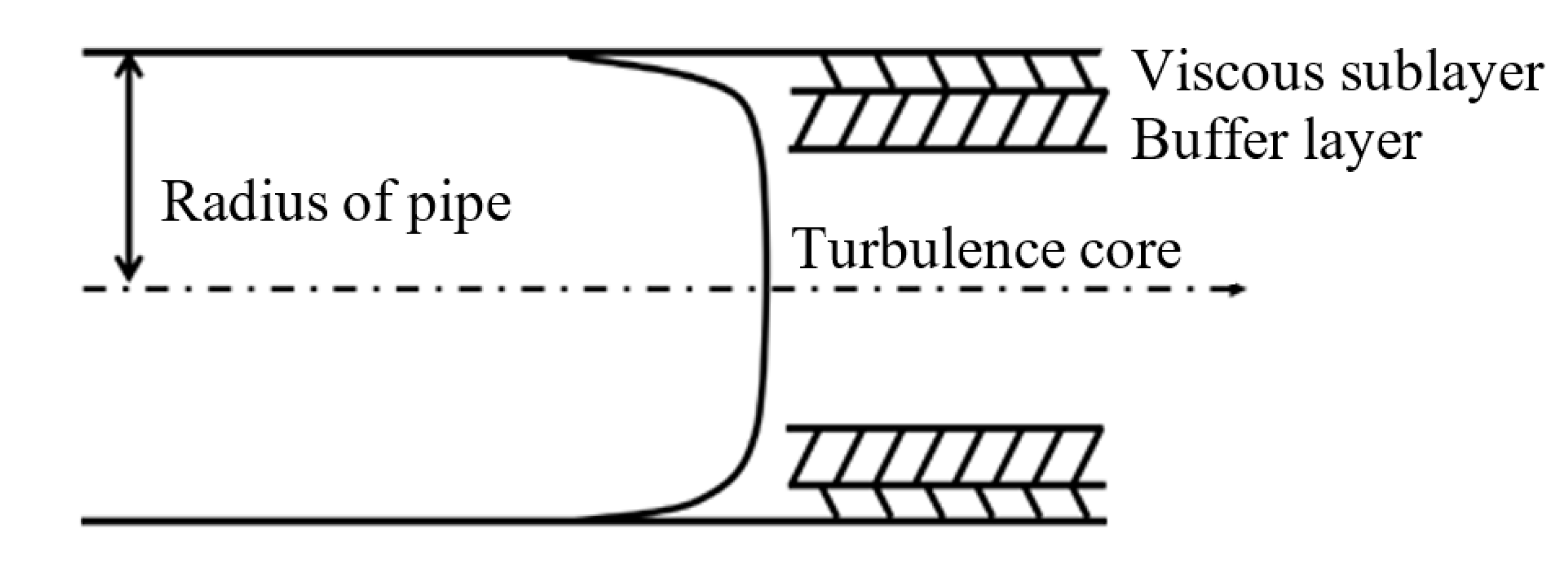
Figure 1. The boundary layer of turbulent flow.
Energies 13 06398 g001
Figure 2. The external node and the control volume in cylindrical coordinate.
Energies 13 06398 g002
Figure 3. The schematic diagram of characteristics method.
Energies 13 06398 g003
Figure 4. Method of calculating deviation volume.
Energies 13 06398 g004
Figure 5. Grid independence test.
Energies 13 06398 g005
Figure 6. Comparison of simulation and experiment.
Energies 13 06398 g006
Figure 7. Comparison of simulation and experiment in pipeline.
Energies 13 06398 g007
Figure 8. Comparison of 2D and 1D model.
Energies 13 06398 g008
Figure 9. Results of 2-dimensional model.
Energies 13 06398 g009
Figure 10. Comparison of concentration distribution of convection term and 2D model.
Energies 13 06398 g010
Figure 11. Comparison of concentration distribution of diffusion term and 2D model.
Energies 13 06398 g011
Figure 12. Diffusion coefficient distribution.
Energies 13 06398 g012
Figure 13. Grid refinement in boundary layer.
Energies 13 06398 g013
Figure 14. Comparison of with and without grid refinement in boundary layer.
Energies 13 06398 g014
Figure 15. Sensitivity analysis map of deviation volume Vd0.5.
Energies 13 06398 g015
Figure 16. Sensitivity analysis map of deviation volume Vd0.1.
Energies 13 06398 g016
Figure 17. Sensitivity analysis map of deviation volume ratio Vd0.1/Vd0.5.
Energies 13 06398 g017
Figure 18. Sensitivity analysis map of length ratio of front and tail part.
Energies 13 06398 g018
Table 1. The density of oil products.
VarietyDensity (kg/m3)Temperature Coefficient (kg/(m3·°C))
15.6 °C17 °C37.8 °C
Gasoline90#733.9732.7713.90.91
95#754.4713.5751.81.84
Diesel0#842.1841.1826.70.69
Table 2. The viscosity of oil products.
VarietyViscosity ( × 10 6   m / s 2 ) Viscosity Temperature Index
15.6 °C17 °C37.8 °C(1/°C)
Gasoline90#0.5940.5870.4890.00877
95#0.5930.4880.5860.00876
Diesel0#6.0815.8673.4520.02550
Publisher’s Note: MDPI stays neutral with regard to jurisdictional claims in published maps and institutional affiliations.