Techno-Economic Assessment of Different Heat Exchangers for CO₂ Capture

Abstract

We examined the cost implications of selecting six different types of heat exchangers as the lean/rich heat exchanger in an amine-based CO₂ capture process. The difference in total capital cost between different capture plant scenarios due to the different costs of the heat exchangers used as the lean/rich heat exchanger, in each case, is in millions of Euros. The gasketed-plate heat exchanger (G-PHE) saves significant space, and it saves considerable costs. Selecting the G-PHE instead of the shell and tube heat exchangers (STHXs) will save €33 million–€39 million in total capital cost (CAPEX), depending on the type of STHX. About €43 million and €2 million in total installed costs (CAPEX) can be saved if the G-PHE is selected instead of the finned double-pipe heat exchanger (FDP-HX) or welded-plate heat exchanger, respectively. The savings in total annual cost is also in millions of Euros/year. Capture costs of €5/tCO₂–€6/tCO₂ can be saved by replacing conventional STHXs with the G-PHE, and over €6/tCO₂ in the case of the FDP-HX. This is significant, and it indicates the importance of clearly stating the exact type and not just the broad classification of heat exchanger used as lean/rich heat exchanger. This is required for cost estimates to be as accurate as possible and allow for appropriate comparisons with other studies. Therefore, the gasketed-plate heat exchanger is recommended to save substantial costs. The CO₂ capture costs of all scenarios are most sensitive to the steam cost. The plate and frame heat exchangers (PHEs) scenario’s capture cost can decline from about €77/tCO₂ to €59/tCO₂ or rise to €95/tCO₂.

1. Introduction

The burning of fossil fuels by power plants and other process industries contributes around half of the world’s CO₂ emissions [1]. These emissions’ adverse effects are evident: the melting of glaziers, deforestation, and droughts in several places [2,3]. With the projected growth of the world’s population, there will be a corresponding increase in the amount of CO₂ emissions. Consequently, human intervention is required for the mitigation of climate change. According to the Intergovernmental Panel on Climate Change (IPCC), the United States Environmental Protection Agency (EPA), and the International Energy Agency (IEA), carbon capture and storage (CCS) is necessary to achieve the 2-degree goal and the 1.5-degree goal of the Paris Agreement [4,5,6].

Several CO₂ capture technologies and methods have been identified. They are based on chemical absorption and desorption using solvents [3], adsorption using solid adsorbent [7], and cryogenic separation that involves the separation of CO₂ by refrigerating and condensing the flue gas consecutively at different condensation temperatures [3,7]. They are also based on membrane separation technology ([3,7], and the direct injection of flue gas into reservoirs of naturally existing methane hydrate to displace methane and form a new CO₂ hydrate [8]. Among these, the amine solvent-based CO₂ absorption and desorption process is the most technologically and commercially matured option [9,10,11,12,13,14,15,16]. However, its industrial deployment requires large investments and an enormous energy supply for desorption [17]. Therefore, it is essential to look into the primary units contributing the most to the capital cost for cost-saving potential. The most expensive units in a standard solvent-based CO₂ capture process are mostly the absorption column and the lean/rich heat exchanger (LRHX), also referred to as the main or cross exchanger. This study focuses on the latter equipment.

Even though the shell and tube heat exchangers (STHX) are the most robust, especially the floating head type [18], and are the most common heat exchangers [18,19,20] in the process industry, there are other types of heat exchangers that are also popular [18,21]. Examples are the plate and frame heat exchangers (PHE) and double-pipe heat exchangers (including finned double-pipe heat exchanger (FDP-HX)). The majority of available CO₂ capture cost studies either do not disclose or merely state the broad classification and not the exact type of heat exchanger employed in the process [1,12,21,22,23]. Examples of broad classifications are shell and tube heat exchangers (STHX) and plate and frame heat exchangers (PHE). However, there are different heat exchangers within these broad classifications, and each has a different cost [18,20,24]. The STHXs have different types of designs and, by implication, different costs and technical advantages [18,20]. Therefore, there is a need to study how each of the popular heat exchangers within their collective classifications affects the process’s cost.

No study has been found where different designs of heat exchangers for CO₂ capture have been examined. This work aims to overview the cost implications of selecting any of six different heat exchangers as the LRHX of the CO₂ capture process. Six different CO₂ capture plant scenarios, each with one of the following heat exchangers as the LRHX, are examined: U-tube shell and tube heat exchangers (UT-STHX) [18,20], fixed tube-sheets shell and tube heat exchangers (FTS-STHX) [18,20], floating head shell and tube heat exchangers (FH-STHX) [18,20], finned double-pipe heat exchangers (FDP-HX) [18,20], and gasketed-plate heat exchangers (G-PHE) and welded-plate heat exchangers (W-PHE) as the LRHX [18,19,20,25]. The technical strength and limitations of these heat exchangers are also reviewed.

Our study could only focus on solvent-based post-combustion CO₂ absorption and desorption process where the lean/rich heat exchanger is an important integral part of the process for heat recovery. Monoethanolamine (MEA) with ~30 wt.% concentration is the standard CO₂ absorption solvent and the most extensively studied solvent [1,12,26,27]. Therefore, it was the solvent used in this study. A typical cement plant flue gas without NOx and Sox is used in this work. This is because the scope of this study does not cover flue gas pre-treatment. It is not necessary because this work focuses on the lean/rich heat exchanger. Cement manufacturing processes, including the combustion of fuel in the manufacturing process, account for 8 percent of global CO₂ emissions, primarily responsible for global warming. Thus, much attention is currently being given to CO₂ capture from the cement industry [12,28,29,30,31,32,33,34,35,36]. The process specifications, including the flue gas composition, are obtained from [11,37] and are given in Table 1. The flue gas contains 25.2 mole% of CO_2, typical of the CO₂ concentrations (22–29%) of flue gas from the clinker production loop [12]. Some previous works on CO₂ capture from cement industry flue gas also primarily focused on these high concentrations of CO₂ from the clinker production loop as done in this work [11,31,38,39,40,41]. Reference [12] covered exhaust gas from both the clinker production loop and fuel combustion. Since this study’s focus is on the main heat exchanger units, the source of flue gas is not important. Another objective is the comprehensive application of the enhanced detailed factor (EDF) method for capital cost estimation, established in Reference [11]. Relevant details of this method are given in Section 2.3 and more comprehensively in Reference [11].

2. Methodology

2.1. Materials and Methods

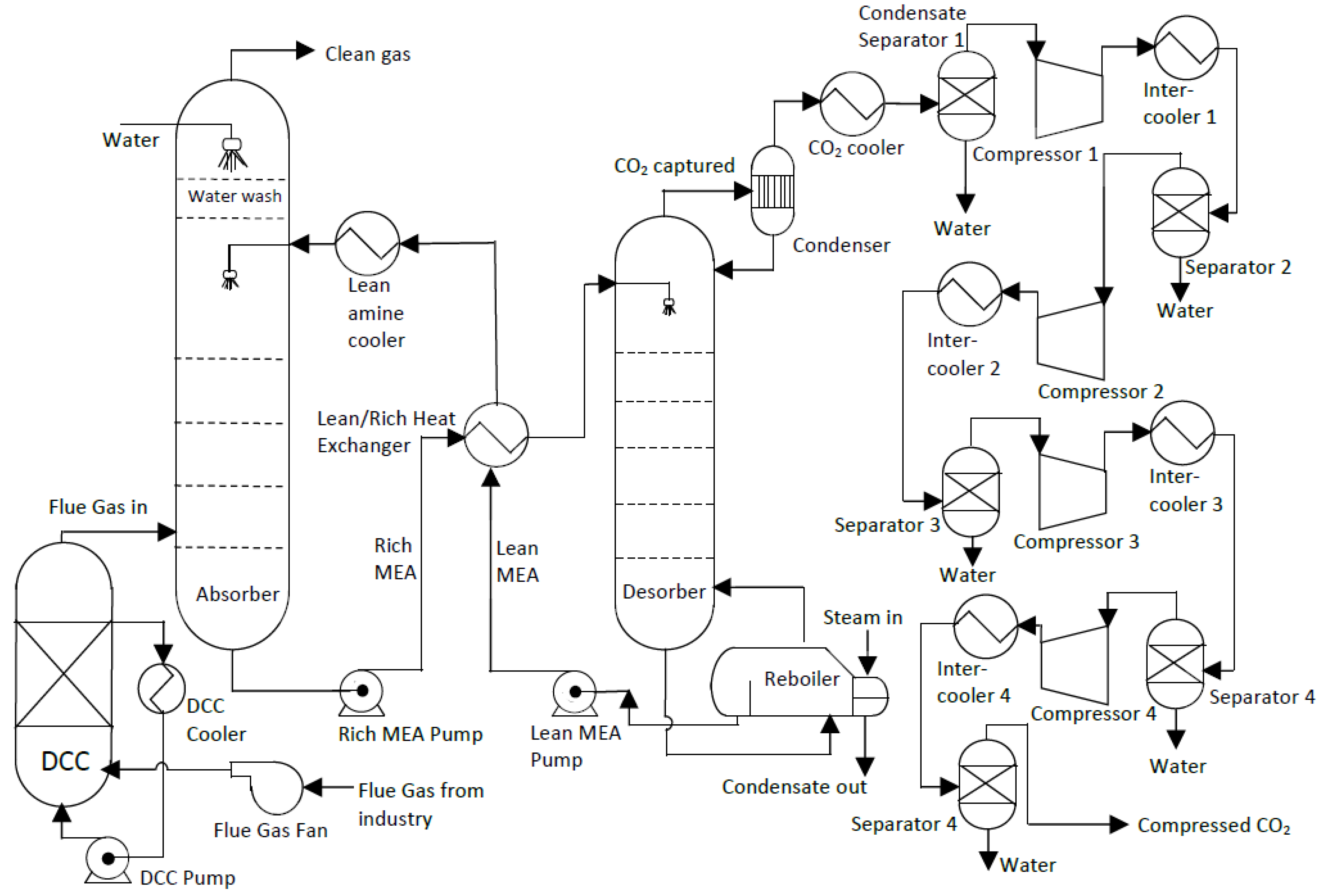
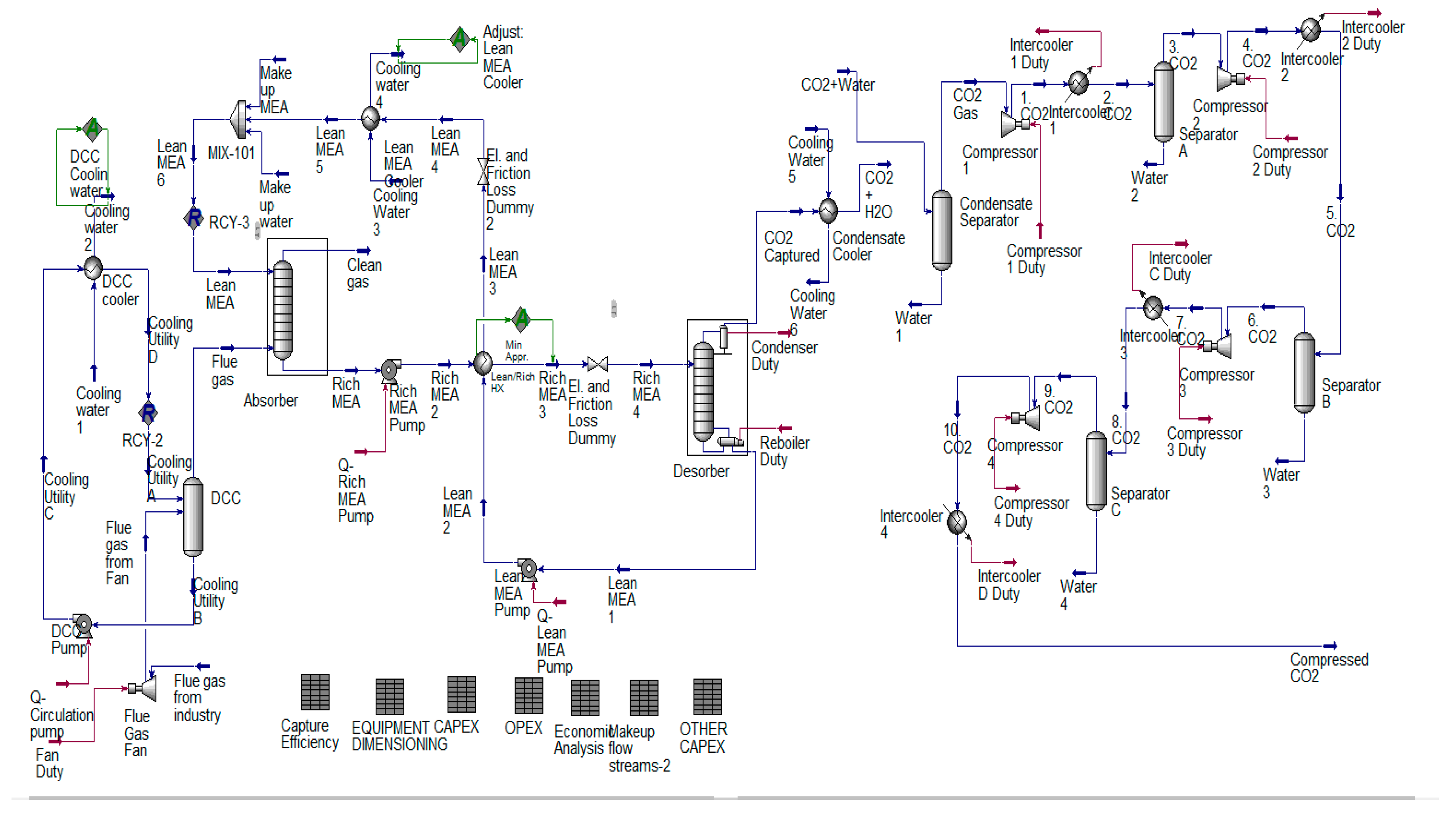
This study is based on the standard or conventional amine-based CO₂ absorption and desorption process. Its simplified process flow diagram (PFD) is shown in Figure 1, and the Aspen HYSYS PFD can be found in Figure A1 in Appendix B. The process can be divided into three parts.

• Pre-capture process and simulation: This is the part of the process before the main CO₂ absorption in the absorber. In order to minimize the complexity of process simulations, flue gas pre-treatment equipment such as a selective catalytic reduction (SCR) unit, flue gas desulfurization (FGD), or baghouse are not included in this work [6]. The equipment considered in this first part of the process is therefore limited to the flue gas fan for the transport of the flue gas to the absorber, through the direct contact cooler (DCC) unit where the flue gas temperature is reduced to 40 °C; the DCC pump for pumping cooling water into the DCC unit; and the DCC cooler to cool the water down to the required temperature.
• Capture process: The relevant equipment includes a simple absorption column and desorption column (stripper) with a condenser and a reboiler, a main heat exchanger (LRHX), two pumps (lean pump and rich pump), and a lean amine cooler. The flue gas from the DCC unit enters the absorber at the bottom of the column where the CO₂ in the flue gas is absorbed into a counter-current flowing amine solvent, which is monoethanolamine (MEA) in this work. An amine solution rich in CO₂ leaves from the bottom of the absorber. The rich pump then pumps it through the LRHX, where it is heated before it flows into the desorber for regeneration. The CO₂ is stripped off the amine solution and leaves through the top of the column and through the condenser. The regenerated solvent, the lean amine, is pumped by the lean pump back to the absorber, but first, through the LRHX to heat the CO₂-rich stream. It is further cooled to 40 °C by a cooler before entering the absorber at the top to continue another absorption cycle. Even though the water wash section is shown in Figure 1, it is not included in this study for simplicity.
• Post capture process: This part of the process involves the compression of the CO₂ to the required utilization pressure. In this study, transport and storage of the compressed CO₂ are not considered. The equipment included are 4 stage-compressors with inter-stage coolers, a CO₂ cooler, and separators [11,12].

2.2. Base Case Process Specifications, Assumptions and Simulation

The mass and energy balances on which equipment sizing was based, as well as utilities consumption used for estimation of variable operating costs, were made available from process simulations. The simulations were performed within the scope of the equipment in Figure 1. The simulations are based on the flue gas specifications given in Table 1. They represent a flue gas of a typical cement plant and are obtained from References [11,37]. The simulation method used in this work was the same as that used in References [42,43]. The difference was that in this work, the simulations were performed using Aspen HYSYS Version 10, where the acid gas property package replaced the Amine property package in previous versions. CO₂ capture of 85% was assumed [28,32,44].

The absorption column and the desorption column were both simulated as equilibrium stages with stage efficiencies (Murphree efficiencies). Each equilibrium stage was assumed to be 1 m high for both columns [11,45]. The industry’s flue gas had a temperature of 80 °C, and it was cooled to 40 °C before entering the absorption column at the bottom at 1.21 bar. The absorber was simulated with 15 packing stages, which was the cost optimum in Reference [17]. Murphree efficiencies of 11–21% were specified from the bottom to the top of the absorption column as in Reference [11]. The desorber was simulated with 10 packing stages, which was also the cost optimum in Reference [17]. For the desorber, a constant Murphree efficiency of 50% for each stage was assumed [11]. The modified HYSIM inside-out algorithm was selected in the columns because it improves convergence [43].

Adiabatic efficiency of 75% was specified for all the pumps and the flue gas fan. The lean pump raised the lean amine stream pressure by 3 bar before passing through the LRHX. Similarly, the rich pump increased the pressure of the CO₂-rich amine solution stream by 2 bar. The minimum approach temperature ($\Delta T_{min}$) in the LRHX was specified as 10 °C [42]. The lean amine cooler further reduced the lean amine stream’s temperature to 40 °C before flowing back into the absorber.

Table 1. Specifications and assumptions for simulation.

Parameter	Value	Source
CO2 capture efficiency (%)	85	[44]
Flue gas
Temperature (°C)	80	[37]
Pressure (kPa)	121	[11]
CO2 mole-fraction	0.2520	[37]
H2O mole-fraction	0.0910	[37]
N2 mole-fraction	0.5865	[37]
O2 mole-fraction	0.0705	[37]
Molar flow rate (kmol/h)	11,472	[37]
Temperature of flue gas into absorber (°C)	40	[43]
Pressure of flue gas into absorber (kPa)	121	[11]
Lean MEA
Temperature (°C)	40	[42]
Pressure (kPa)	121	[11]
Molar flow rate (kmol/h)	96,850	Calculated
Mass fraction of MEA (%)	29	[42]
Mass fraction of CO2 (%)	5.35	[42]
Absorber
No. of absorber stages	15	[17]
Absorber Murphree efficiency (%)	11–21	[11]
ΔTmin lean/rich heat exchanger (°C)	10	[12,42]
Desorber
Number of stages	10	[17]
Desorber Murphree efficiency (%)	50	[11]
Pressure (kPa)	200	[42]
Reflux ratio in the desorber	0.3	[42]
Temperature into desorber (°C)	104.6	[43]
Reboiler
Reboiler temperature (°C)	120	[42]
Saturated steam temperature (°C)	160	[46]
Exit temperature of steam (°C)	151.8	[46]
CO2 compression final pressure (kPa)	15,100	[47,48]

Table 1. Specifications and assumptions for simulation.

Parameter	Value	Source
CO2 capture efficiency (%)	85	[44]
Flue gas
Temperature (°C)	80	[37]
Pressure (kPa)	121	[11]
CO2 mole-fraction	0.2520	[37]
H2O mole-fraction	0.0910	[37]
N2 mole-fraction	0.5865	[37]
O2 mole-fraction	0.0705	[37]
Molar flow rate (kmol/h)	11,472	[37]
Temperature of flue gas into absorber (°C)	40	[43]
Pressure of flue gas into absorber (kPa)	121	[11]
Lean MEA
Temperature (°C)	40	[42]
Pressure (kPa)	121	[11]
Molar flow rate (kmol/h)	96,850	Calculated
Mass fraction of MEA (%)	29	[42]
Mass fraction of CO2 (%)	5.35	[42]
Absorber
No. of absorber stages	15	[17]
Absorber Murphree efficiency (%)	11–21	[11]
ΔTmin lean/rich heat exchanger (°C)	10	[12,42]
Desorber
Number of stages	10	[17]
Desorber Murphree efficiency (%)	50	[11]
Pressure (kPa)	200	[42]
Reflux ratio in the desorber	0.3	[42]
Temperature into desorber (°C)	104.6	[43]
Reboiler
Reboiler temperature (°C)	120	[42]
Saturated steam temperature (°C)	160	[46]
Exit temperature of steam (°C)	151.8	[46]
CO2 compression final pressure (kPa)	15,100	[47,48]

The captured CO₂ undergoes a four stages compression with inter-stage cooling [11,12]. The final pressure is 151 bar with a purity of 99.8%, which is 0.17% less than [47] with 90% CO₂ capture. This was consistent with the requirements for enhanced oil recovery (EOR) and/or offshore geological sequestration [12,31,38,48,49]. The major uses of the compressed CO₂ include EOR, coalbed CH₄ recovery, and injection into un-minable coal seams or deep saline formation [48]. A potential future application is the injection of the CO₂ (especially in mixture with nitrogen) into naturally existing methane hydrate reservoirs for simultaneous CH₄ production and storage of CO₂ in the form of hydrate [48,50,51,52,53]. The compressed CO₂ pressure is expected to be 110–152 bar [48,49,54]. A similar assumption (150 bar) was made by References [12,21,31,47]. The following studies assumed 110 bar [28,29,55]. The final pressure depends on the transport distance between the CO₂ capture plant and the sequestration site/utilization point.

2.3. Capital Cost Estimation Method

When equipment cost data are available, a factorial method of capital cost estimation can be applied. Various forms of factors or factorial schemes are available, from Lang Factors [56], Hand Factors [57], to more detailed factors found in References [58,59], and more recently in References [60] and in [11]. Most of the factorial methods are based on the work of References [58,59]. The most popular of them is the methodology documented by the National Energy Technology Laboratory (NETL) [61], which is used for capital cost estimation in [62].

In this work, the enhanced detailed factor (EDF) method, which is comprehensively documented in Reference [11], was applied to estimate the total capital cost/CAPEX. This has the same strategy as the individual factor and subfactor estimating method in Reference [60]. However, the EDF method’s installation factors are more detailed [11]. The EDF cost estimation scheme developed by Nils Eldrups at SINTEF Tel-Tek and the University of South-Eastern Norway (USN) has been used extensively in these Norwegian institutions for several years.

The EDF method was chosen for this work because the installation factors for all equipment pieces, irrespective of their sizes and cost, cannot be the same [60] as they are treated in most of the other methods already mentioned. Applying individual installation factors to an individual piece of equipment improves capital cost estimates [60]. Therefore, the EDF method’s merits include higher accuracy of cost estimates in the early stage, highlighting an individual piece of equipment for optimization [11]. Individual installation factors are applied to each separate unit of equipment, thereby handling each individual equipment as a separate project. This eventually improves the accuracy of capital cost estimates. The EDF cost estimation method gives a high level of accuracy in the early-stage chemical plant cost estimates. In addition, it can easily and straightforwardly be employed to implement cost engineering studies of new technologies or retrofits (extension) or modifications of projects for an existing chemical plant [11].

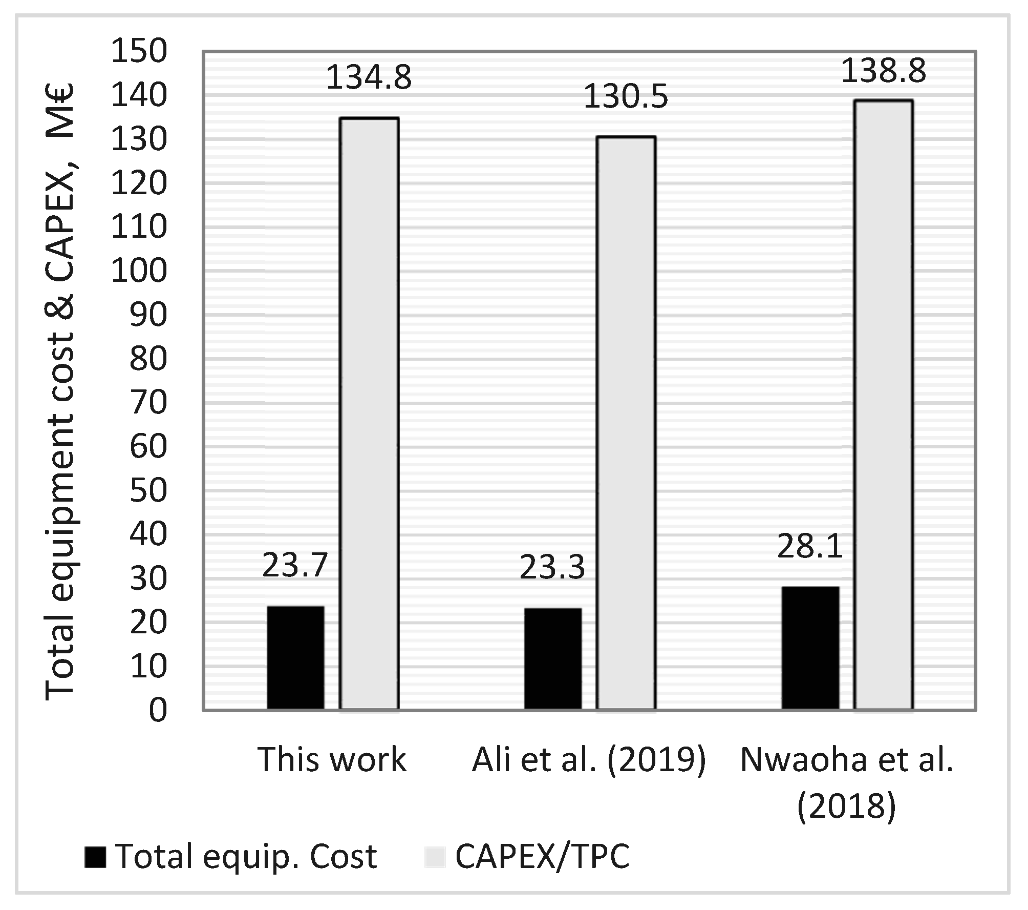
The total installed cost (CAPEX) estimated using the EDF scheme corresponds to the total plant costs (TPC) using the methodology of NETL. It is important to emphasize that the EDF method does not consider the cost escalations and interest accrual during the construction period, the costs for land purchase and preparation, long pipelines, long belt conveyors, office buildings, and workshops, and other costs incurred by the owner.

2.4. Scope of Capital Cost Estimation

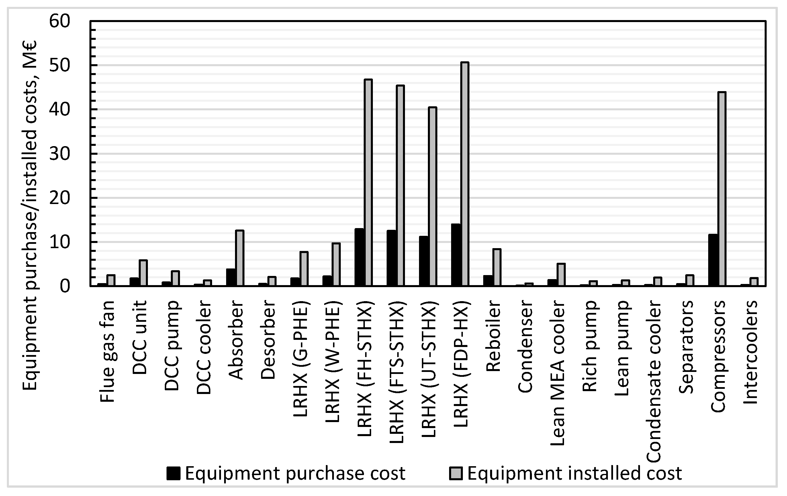
The equipment considered in this work included the (1) flue gas fan, (2) direct contact cooler (DCC Unit), (3) DCC pump, (4) DCC cooler, (5) absorber, (6) desorber, (7) condenser, (8) reboiler, (9) lean/rich heat exchanger (LRHX), (10) lean MEA cooler, (11) lean pump, (12) rich pump, (13) condensate cooler, (14) compressors (×4), (15) inter-stage cooler (×4), and (15) Separators (×4). Some other types of equipment that were not included in this study but are vital for the operation and performance of this type of plant were (1) water wash section, (2) MEA reclaimer, (3) equipment for conditioning of make-up MEA and make-up water, and (4) cooling water pumps for DCC cooler, condensate cooler and inter-stage coolers. In addition, the cost of acquiring the site (land), preparing the site, and service buildings are not included.

2.5. Equipment Dimensioning and Assumptions

Mass and energy balances from the process simulations are used for sizing the equipment listed above. The dimensioning approach is the same for previous studies at USN [11,17,55]. The dimensioning factors and assumptions are summarised in Table 2. Since CO₂ is an acid gas with a risk of corrosion, stainless steel SS316 is assumed for all equipment except the flue gas fan and compressor casings, which are assumed to be manufactured from carbon steel.

Even though the water wash section is not included in the cost estimate, the tangent-to-tangent height (TT) of the absorber is assessed to cover the water-wash requirements, demister, packing, liquid distributors, gas inlet and outlet, and sump [11]. Similarly, the packing requirements, liquid distributor, gas inlet, inlet for the condenser, and sump are accounted for in evaluating the tangent-to-tangent height (TT) of the desorption column [11].

The heat transfer area required is the key design parameter in the initial cost estimate of the general heat transfer equipment. These include the LRHX, reboiler, condenser, and coolers. The heat transfer area is computed from the heat duty (heat transfer from hot to cold stream), overall heat transfer coefficient, and the log-mean temperature difference (LMTD) [63]. The overall heat transfer coefficient (U-value) assumed for the lean/rich heat exchanger scenarios with the STHXs and FDP-HX is 500 W/m²K [45]. This value is close to the 550 W/m²K used by SINTEF (a research organization in Norway) [64]. The overall heat transfer coefficient for the PHEs was conservatively assumed to be 1000 W/m²K. This is because the overall heat transfer coefficient of the PHEs is much higher than that of other exchangers like the STHXs, thereby having an order of magnitude higher surface area per unit volume compared to the STHXs [18,19]. According to Reference [65], the U-value for the PHEs is 2–4 times the STHXs. The welded-plate heat exchanger was assumed to cost 25% more than the gasketed-plate heat exchanger based on information from Reference [18].

The flowrate and power (duty) of each pump, compressor, and flue gas fan were obtained directly from the Aspen HYSYS simulation. The separators were sized from gas flowrate, mass densities of the gas and liquid phases, using the Souders-Brown Equation with a k-factor of 0.101 m/s [66,67]. The wall thickness determination followed the typical format, with joint efficiency of 0.8, corrosion allowance of 0.001 m, and stress of 2.15 × 10⁸ Pa. The design pressure was obtained from Aspen HYSYS. After evaluating the vessel’s outer diameters (D_o), the TT was estimated from the assumption of TT = 3D_o. The dimensions and purchase costs of all the equipment are given in

Table A2. Columns and pressure vessel dimensions and purchase costs from Aspen In-Plant Cost Estimator V11 (purchased cost year: 2018).

		Material	Outer Diameter	Tangent-to-Tangent Height	Purchase Cost
			(m)	(m)	(1000 × €)
Absorber	Shell	SS316	6.58	40	2046
	Packing (structured)	Mellapack M250YB	6.51	15	1765
Desorber	Shell	SS316	2.24	25	389
	Packing (structured)	Mellapack M250YB	2.2	10	128
DCC unit	Shell	SS316	4.94	15	1766
	Packing (structured)	Mellapack M250YB		4
Separator 1		SS316	2.79	8.4	156
Separator 2		SS316	2.05	6.2	96
Separator 3		SS316	1.59	4.8	108
Separator 4		SS316	1.15	3.5	121.3

,

Table A3. Pumps dimensions and purchase costs from Aspen In-Plant Cost Estimator V11 (purchased cost year: 2018).

	Material	Flowrate	Duty	No. of Units	Purchase Cost/Unit
		(L/s)	(kW)	(-)	(1000 × €)
DCC pump	SS316	1828.8	438.9	1	855.9
Rich pump	SS316	658.4	244.9	1	212.9
Lean pump	SS316	694.9	278.0	1	250.9

,

Table A4. Heat exchange equipment dimensions and purchase costs from Aspen In-Plant Cost Estimator V11 (purchased cost year: 2018).

	Material	Total Heat Transfer Area	No. of Units	Purchase Cost/Unit
		(m2)	(-)	(1000 × €)
LRHX (UT-STHX)	SS316	963.5	23	485.3
LRHX (FTS-STHX)	SS316	963.5	23	544.5
LRHX (FH-STHX)	SS316	963.5	23	561.0
LRHX (FDP-HX)	SS316	886.4	25	558.8
LRHX (G-PHE)	SS316	1477.3	15	235.4
Reboiler (Kettle-type)	SS316	974.5	4	579.3
Lean MEA cooler (UT-STHX)	SS316	938.2	3	468.5
DCC cooler (UT-STHX)	SS316	699.7	1	366.8
Condenser (UT-STHX)	SS316	193.4	1	118.5
Condensate cooler (UT-STHX)	SS316	420.1	1	248.8
Intercooler 1 (UT-STHX)	SS316	105.6	1	70.3
Intercooler 2 (UT-STHX)	SS316	62.6	1	49.7
Intercooler 3 (UT-STHX)	SS316	72.2	1	58.6
Intercooler 4 (UT-STHX)	SS316	109.6	1	130.4

and

Table A5. Compressors and flue gas fan dimensions and purchase costs from Aspen In-Plant Cost Estimator V11 (purchased cost year: 2018).

	Material	Inlet Pressure	Outlet Pressure	Gas Flowrate	Duty	Purchase Cost/Unit
		(bar)	(bar)	(m3/h)	(kW)	(1000 × €)
Compressors 1	CS	1.5	4.8	48,418	3549	5320.2
Compressors 2	CS	4.3	13.76	14,523	3053	2436.9
Compressors 3	CS	13.26	46.41	4447	3137	1904.5
Compressors 4	CS	45.91	151.1	1014	2437	1981.8
Flue gas fan	CS	1.01	1.21	333,126	2305	482.4

in Appendix C.

Table 2. Equipment dimensioning factors and assumptions.

Equipment	Basis/Assumptions	Sizing Factors
DCC Unit	Velocity using Souders-Brown equation with a k-factor of 0.15 m/s [66]. TT =15 m, 1 m packing height/stage (4 stages) [11]	All columns: Tangent-to-tangent height (TT), Packing height, internal and outer diameters (all in (m))
Absorber	Superficial velocity of 2 m/s, TT=40 m, 1 m packing height/stage (15 stages) [11,17]
Desorber	Superficial velocity of 1 m/s, TT=22 m, 1 m packing height/stage (10 stages) [11,17].
Packings	Structured packing: SS316 Mellapak 250YB	See DCC Unit, absorber and desorber
Lean/rich heat exchanger	U = 0.5 kW/m2K [45]	Heat transfer area, A (m2)
Reboiler	U = 0.8 kW/m2K [45]
Condenser	U = 1.0 kW/m2K [45]
Coolers	U = 0.8 kW/m2K [45]
Intercooler pressure drop	0.5 bar [20]	U-tube HX
Pumps	Centrifugal	Flowrate (L/s) and power (kW)
Flue gas fan	Centrifugal	Flow rate (m3/h)
Compressors	Centrifugal; 4-stages [11,12,54]; Final pressure = 151 bar [48,49]; pressure ratio = 3.2	Power (kW) and flowrate (m3/h)
Separators	Vertical vessels; vessel diameter using Souders-Brown equation, a k-factor of 0.101 m/s [66,67]; corrosion allowance of 0.001 m; joint efficiency of 0.8; stress of 2.15 × 108 Pa [45]; TT = 3Do [67]	Outer diameters (Do); tangent-to-tangent height (TT), (all in (m))

Table 2. Equipment dimensioning factors and assumptions.

Equipment	Basis/Assumptions	Sizing Factors
DCC Unit	Velocity using Souders-Brown equation with a k-factor of 0.15 m/s [66]. TT =15 m, 1 m packing height/stage (4 stages) [11]	All columns: Tangent-to-tangent height (TT), Packing height, internal and outer diameters (all in (m))
Absorber	Superficial velocity of 2 m/s, TT=40 m, 1 m packing height/stage (15 stages) [11,17]
Desorber	Superficial velocity of 1 m/s, TT=22 m, 1 m packing height/stage (10 stages) [11,17].
Packings	Structured packing: SS316 Mellapak 250YB	See DCC Unit, absorber and desorber
Lean/rich heat exchanger	U = 0.5 kW/m2K [45]	Heat transfer area, A (m2)
Reboiler	U = 0.8 kW/m2K [45]
Condenser	U = 1.0 kW/m2K [45]
Coolers	U = 0.8 kW/m2K [45]
Intercooler pressure drop	0.5 bar [20]	U-tube HX
Pumps	Centrifugal	Flowrate (L/s) and power (kW)
Flue gas fan	Centrifugal	Flow rate (m3/h)
Compressors	Centrifugal; 4-stages [11,12,54]; Final pressure = 151 bar [48,49]; pressure ratio = 3.2	Power (kW) and flowrate (m3/h)
Separators	Vertical vessels; vessel diameter using Souders-Brown equation, a k-factor of 0.101 m/s [66,67]; corrosion allowance of 0.001 m; joint efficiency of 0.8; stress of 2.15 × 108 Pa [45]; TT = 3Do [67]	Outer diameters (Do); tangent-to-tangent height (TT), (all in (m))

2.6. Source of Equipment Purchase Costs

The best source of the purchase cost of a piece of equipment is from quotations directly from equipment vendors or equipment manufacturers. This is usually not easy to obtain, and they may also require comprehensive design details. The next best option to this is cost data of the same equipment recently purchased. This kind of cost data may never be accessible to research cost engineers. Therefore, they must rely on either in-house cost data that may not be necessarily very recent or on commercial databases such as Aspen In-plant Cost Estimator from AspenTech, which is the most popular. This AspenTech database was developed by a team of cost engineers based on data obtained from equipment manufacturers and EPC companies. These cost data are updated every year; thus, they are recent and reliable [20]. This study’s cost data were obtained from the most recent Aspen In-plant Cost Estimator Version 11 with the cost year of 2018 January. Therefore, the purchase costs of equipment in this course are updated.

When cost engineers or researchers do not have access to licenses of such databases that are regularly updated, they can use data in the open literature. Some of these data are available as cost correlations in the form of tables or graphs for several types of equipment, some of which can be found in References [18,20,62]. A free internet equipment cost database with a cost period of January 2002 is available in Reference [68].

2.7. Capital Cost Estimation Assumptions

The economic assumptions used for estimating the total capital cost (CAPEX) and annualized CAPEX in the EDF method [11] are given in

Table 3. Assumptions for capital cost estimation.

Parameter	Value	Source
Cost year	2020, January	Assumed
Cost currency	Euro (€)	Assumed
Method of CAPEX estimation	EDF method	[11]
Plant location	Rotterdam	Default
Project life	25 years	[61]
Duration of construction	2 years	Assumed
Discount rate	7.50%	[11]
Material conversion factor (SS to CS)	1.75 Welded; 1.30 machined	[11]
Annual maintenance	4% of CAPEX	[41]
FOAK or NOAK	NOAK	[11]
Cost data year	2018, January	AspenTech-A.I.C.E.
Cost index for January 2020	111.3	[69]
Cost index for January 2018	106.0	[69]
Currency conversion (€ to NOK)	10.13, 25 January 2020	[70]
Currency conversion (US$ to NOK)	9.10, 27 January 2020	[70]
Main economic analysis criteria	CO2 captured cost	[45]
CO2 avoided cost/CO2 captured cost	CO2 captured cost	[11]

. Equipment costs are obtained in Euros (€) and are converted to Norwegian kroner (NOK) to use the installation factors developed in NOK. A brownfield project is assumed. The installation factors are provided in CS; therefore, Equation (1) is applied to convert equipment purchase costs from stainless steel (SS) to CS. The list of installation factors is attached in Appendix A.

$$Equip. purchase cos{t}_{CS}=\frac{Equip. purchase Cos{t}_{\left(SS, exotic,\dots \right)}}{f_{mat}}$$

(1)

When the appropriate detailed installation factors for each piece of equipment is obtained, Equations (2) and (3) can be used to calculate the installed cost of any equipment in CS (flue gas fan and compressors in this work):

$$Equip. installed Cos{t}_{CS} \left(\mathrm{NOK}\right)=Equipment Cos{t}_{CS} \left(\mathrm{NOK}\right)\times F_{Total, CS}$$

(2)

$$F_{Total,CS}= f_{direct}+f_{engg}+f_{administration}+f_{commissioning}+f_{contingency}$$

(3)

Installed costs of equipment manufactured from SS are obtained from Equations (4) and (5):

$$Equip. installed Cos{t}_{\left(SS, exotic,\dots \right)} \left(\mathrm{NOK}\right)=Equipment Cos{t}_{CS} \left(\mathrm{NOK}\right) \times F_{Total, SS, exotic\dots }$$

(4)

$$F_{Total, SS,exotic\dots }=\left(F_{Total, CS}+\left(\left(f_{mat}-1\right)\left(f_{equip}+f_{piping}\right)\right)\right)$$

(5)

The individual piece of equipment’s installed costs is then converted back to €. The installed costs are escalated to January 2020 using the Norwegian Statistisk Sentralbyrå industrial cost index (2018 = 106; 2020 = 111.3) [40].

$$Cos{t}_{2020}= Cos{t}_{2018}\left(\frac{Cost inde{x}_{2020}}{Cost inde{x}_{2018}}\right)$$

(6)

The sum of all the equipment installed costs in 2020 is the plant total installed cost (CAPEX). The annualized CAPEX is evaluated using Equations (7) and (8):

$$Annualised CAPEX \left(\frac{€}{yr}\right) =\frac{CAPEX}{Annualised factor}$$

(7)

The annualized factor is calculated, as shown in Equation (8):

$$Annualised factor= {\displaystyle \sum }_{i=1}^{23}\left[\frac{1}{{\left(1+r\right)}^n}\right]$$

(8)

where n represents operational years and r is discount/interest rate for a 2-year construction period and 23 years of operation.

2.8. Operating and Maintenance Costs (O&M or OPEX) and Assumptions

The operating and maintenance costs (O&M) are mainly referred to as OPEX, operating expenses. These costs are usually divided into fixed operating costs and variable operating costs. Fixed operating costs are operating costs that do not vary in the short term and do not depend on the units of materials consumed or produced. Fixed operating costs do not depend on how much CO₂ is captured. The fixed operating costs in this work followed the assumptions used in Reference [11]. They only include:

• Maintenance costs.
• Labor costs (Salary for 1 Engineer and 6 Operators).

Maintenance cost in this study is estimated as follows [33]:

$$Mtce cost=0.04\times \left(installed cost of all equipment or CAPEX\right)$$

(9)

Variable operating costs are the operating expenses that vary with either the units of materials consumed or produced. These are mainly utilities and raw materials. In this study, they are limited to:

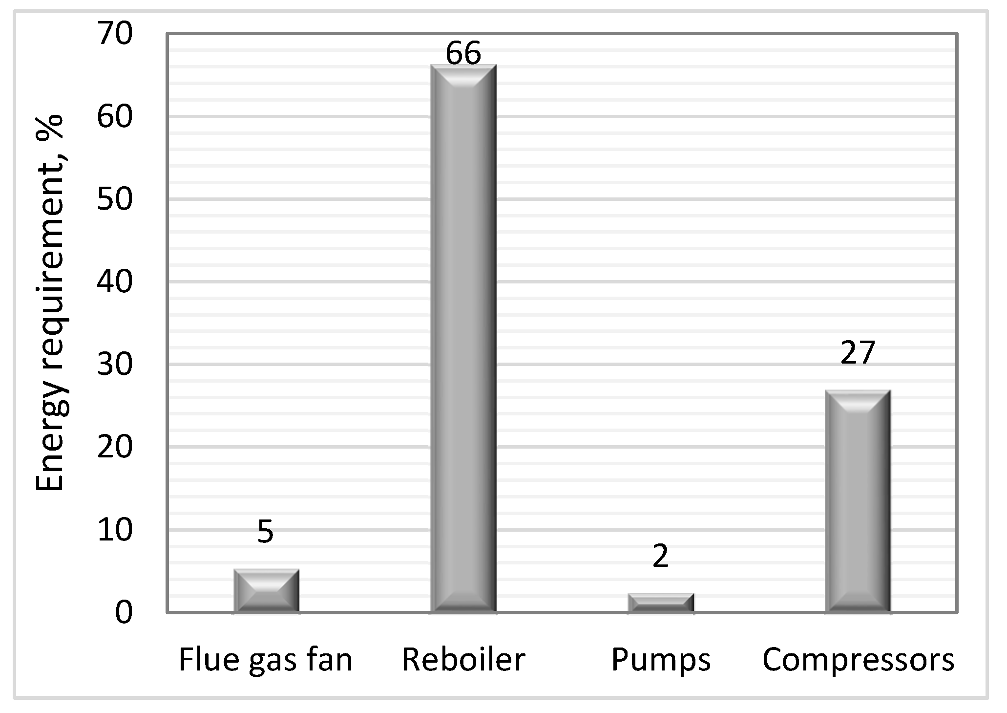
• Cost of electricity consumed by the flue gas fan, pumps, and compressors
• Cost of steam consumption in the reboiler.
• Cost of cooling water required by the coolers.
• Cost of process (demineralized) water in the amine solution solvent and make-up water.
• Cost of solvent.

Each variable operating cost is estimated using Equation (10):

$$Variable operating cost \left(\frac{€}{yr}\right)=Consumption\left(\frac{unit}{hr}\right) \times unit price\left(\frac{€}{unit}\right)\times operational hours\left(\frac{hr}{yr}\right)$$

(10)

where the unit for electricity and steam consumption is kWh. The unit for all water and solvent is m³. The assumptions for the fixed operating costs and unit prices of the variable operating costs are given in

Table 4. Operating cost data.

	Unit	Value/unit *	Reference
Steam	€/kWh	0.032	[22]
Electricity	€/kWh	0.132	[11]
Cooling water	€/m3	0.022	[11]
Water (process) *	€/m3	0.203	[71]
MEA	€/m3	2,069	[11]
Maintenance	€	4% of CAPEX	[71]
Operator	€	85,350 (× 6 operators)	[11]
Engineer	€	166,400 (1 engineer)	[11]

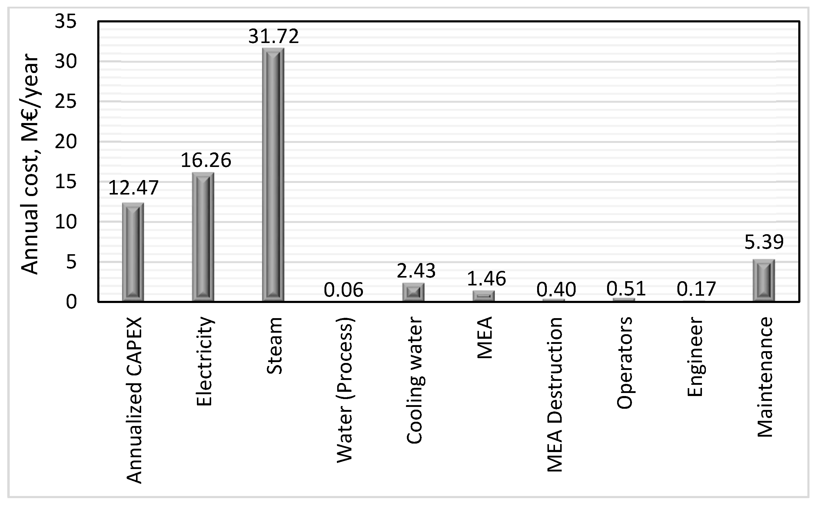
* The costs have been escalated to January 2020.

. These costs are updated to 2020 from the references. The total annual operating expenses (annual OPEX) is the sum of all the annual costs of fixed operating costs and variable operating costs. Costs for CO₂ transport and storage, pre-production costs, insurance, taxes, first fill cost, and administrative costs are not included in the OPEX.

2.9. Total Annual Cost and CO₂ Captured Cost

Total Annual Cost and CO₂ capture Cost are the bases for techno-economic analysis in this work. The total annual cost is simply the sum of annualized CAPEX and yearly total operating cost as given in Equation (11):

$$Total Annual Cost\left(\frac{€}{yr}\right)= Annualized CAPEX \left(\frac{€}{yr}\right)+Annual OPEX \left(\frac{€}{yr}\right)$$

(11)

Most literature reports their results in CO₂ avoided cost [72,73], and CO₂ captured cost [74]. Therefore, it was important to perform our estimates with similar cost metrics for comparison with other works. In this study, results are reported in CO₂ capture cost and total annual cost. In this work, different scenarios of CO₂ capture plants with different heat exchanger types were compared. CO₂ captured cost is the annual cost per ton or per kmol of CO₂ captured as expressed in Equations (12) and (13):

$$C{O}_{2}captured cost \left(\frac{€}{t C{O}_2}\right)=\frac{Total Annual Cost \left(TAC\right) \left(\frac{€}{yr}\right)}{Mass ofC{O}_2 captured \left(\frac{t}{yr}\right)}$$

(12)

$$C{O}_{2}captured cost\left(\frac{€}{kmol C{O}_2}\right)=\frac{Total Annual Cost \left(TAC\right) \left(\frac{€}{yr}\right)}{Molar flow ofC{O}_2 \left(\frac{kmol}{yr}\right)}$$

(13)

3. Results and Discussion

3.1. Simulation Results

Prior to the CO₂ capture process’s techno-economic analysis, it is essential to validate the process simulation results by comparing them with existing studies.

Table 5. Process simulation results-comparison with literature.

	Capture Efficiency (%)	$\mathbf{\Delta }{\mathit{T}}_{\mathit{m}\mathit{i}\mathit{n}} (\mathbf{°}\mathbf{C})$	Lean Loading	Rich Loading	Absorber Packing Height (m)	Reboiler Heat (GJ/tCO2)
This work	85.04	5	0.26	0.47	15	3.83
	85.03	10	0.26	0.47	15	4.08
Ali et al. [11]	84.92	5	0.26	0.47	15	3.82
	84.78	10	0.25	0.48	15	3.91
Alie et al. [38]	85.00	n.a.	0.25	0.50	n.a	4.02
Kothandaraman [75]	85.00	10	0.25	0.50	17	4.25
Nwaoha et al. [12]	90.00	10	0.25	0.50	22 (36 stages)	3.86
Stec et al. [76]	84.00	n.a.	0.36	0.50	9.2	3.98
Just [75] (Pilot-test)	90.00	n.a.	n.a.	n.a.	11	4.0

n.a. = not available.

presents the lean loading, rich loading, and the reboiler heat consumption from this work and References [11,12,26,38,75,76]. The assumptions and specifications, including the flue gas composition (see Table 1) used in this work are the same as Reference [11]. Both studies have almost the same lean loading and rich loading. The reboiler heat calculated in this work was only 0.15% higher than Reference [11], with $\Delta T_{min}$ of 5 °C in the LRHX. This slight difference was due to the slight difference in CO₂ removal efficiency, as can be observed in Table 5. The reboiler heat consumption in this study was about 4% more than Reference [11] when the $\Delta T_{min}$ of the LRHX was set at 10 $°\mathrm{C}$. This difference was also mainly because of the difference in the CO₂ removal grade. A hypothetical exhaust gas composition of 25 mole% of CO₂ and 75 mole% of N₂ was assumed by Reference [38]. Compared to Reference [75], the results are for flue gas from a coal-fired power plant, which is assumed to consist of 12–14 mole% of CO₂. The exhaust gas composition in the case of Reference [12] is 11.5 vol.%, 65.31 vol.%, 13.17 vol.%, and 10 vol.% of CO₂, N₂, H₂O, and O_2, respectively, together with 198 ppm NOx and 170 ppm Sox. The flue gas composition in Reference [76] is 13.5 volume%, 5.5 vol.%, and 11vol.% of CO₂, H₂O, and O_2, respectively. Three different CO₂ concentrations, 3–5 vol.% (combined-cycle gas turbine (CCGT) applications), 13 vol.% (coal combustion) and 22 vol.% (specific applications like blast furnaces) were tested in laboratory and pilot plants for 90% CO₂ capture. The calculated reboiler heat consumption for the MEA cases in Reference [76] was 3.5–4.5 GJ/kg CO₂. These values were for the absorber with intercoolers. It was a 4.6 GJ/kg CO₂ standard absorber.

Despite concentration differences of CO₂ in flue gas and absorption packing heights, this work’s results were close to the results of the other references in Table 5. The range of reboiler heat demands published in the literature for the standard case with $\Delta T_{min}$ of 10 °C is 3.2–5.0 GJ/t CO₂ [12]. Therefore, the results in this study are relevant for techno-economic analysis.

3.2. Capital Cost of the Base Case

The total capital expenditure or total investment cost (CAPEX) in this study was the sum of the installed costs of all the equipment listed in Section 2.7 (EDF method). The installed cost of each equipment and the CAPEX were estimated using Equations (1)–(6). The base case had UT-STHX as the LRHX with $\Delta T_{min}$ of 10 °C. The base case CAPEX was estimated to be €134.8 million, with a cost period of January 2020.

Figure 2 presents a comparison of the estimated CAPEX with two other studies of amine-based CO₂ capture from a cement plant flue gas [11,12]. The same flue gas specification and similar process and economic assumptions were used in the study published in Reference [11]. The study estimated the CAPEX to be €131 million (updated to January 2020). The difference in CAPEX between this study and Reference [11] resulted from the cost of compressors due to higher final CO₂ compression pressure and the inclusion of the four separators’ cost in this study. The 4-stage compression was also assumed in Reference [11] as done in this work. The final compressor’s outlet pressure was 96 bar, but in this work, it was 151 bar [49]. Therefore, the purchase cost in this work was 1.7% higher than that of Reference [11].

The CAPEX in Reference [12] was estimated at €138.8 million (updated to January 2020); however, the CO₂ capture rate was 90%. They obtained their equipment cost data from vendors and original equipment manufacturers (OEM). They also assumed that all equipment was manufactured from stainless steel (SS316). In this work and Reference [11], the flue gas fan and the compressors’ casing material were assumed to be made from carbon steel. In Reference [12], other cooling water pumps for the condenser, four intercoolers, lean amine cooler, and clean gas cooling were included, which were not included in this study since the focus is on the LRHX. The additional equipment together with the material of construction of the compressors’ casing and blower rather than the source of equipment cost data may be the main reason for the 18.6% higher total equipment cost in Reference [12]. That implies that the total equipment costs obtained directly from vendors and OEM are close to those of this work obtained from Aspen In-plant Cost Estimator version 11.

The EDF method applied for estimating the total capital investment (CAPEX) in this work applied distinct installation factors to each piece of equipment, unlike the method developed by Reference [12] based on the methodology published in References [61,62]. The ratio of CAPEX to total equipment costs in this work was 5.68. In [11], it is 5.59, and in Reference [12], it is 4.94 for the MEA system and 5.46 for the AMP-PZ-MEA process. These values show that applying the Lang factor value of 4.74 (for fluids processing plants) will not yield very good results in preliminary cost estimation [56]. The CAPEX in this work was 3.3% higher than that of Reference [11], and that of Reference [12] was 2.9% higher than this work. The LRHX is the equipment of interest in this work, and it is the second most expensive equipment in the process. It accounts for 30% of the CAPEX.

3.3. Total Annual Operating and Maintenance Costs (O&M)

The total annual operating and maintenance (O&M) costs estimated for the base case in this study was €58 million/year. This consisted of an annual fixed operating cost of €6 million/year, of which the annual maintenance cost was €5 million/year, and the variable operating cost was €52 million/year. The maintenance cost was estimated using Equation (9), and Equation (10) was used to estimate the variable operating costs. The annual OPEX in this study was 11% higher than Reference [11]. The reason was that the unit cost of steam [22] in this study was higher. In addition, the maintenance cost due to the higher CAPEX was more in this study. Figure 3 shows the proportions of energy consumption by different equipment. Steam consumption in the reboiler accounts for 66% of energy consumption. In Reference [26], steam consumption accounted for 60% of energy consumption. Electricity consumption accounts for the remaining 34%, of which the compressors account for 27%.

3.4. Total Annual Cost of the Base Case

The total annual cost for the base case was estimated using Equation (11). The total annual cost was estimated to be €71million/year, of which the annualized CAPEX is €13 million/year. The annualized CAPEX was evaluated using Equations (7) and (8). The annualized factor for 25 years of plant life with a two-year construction period was 10.81. An overview of the total annual cost is given in Figure 4. The highest contribution to the total annual cost was the cost of steam consumption as expected, and it was 45% of the total annual cost. Steam consumption in Reference [11] accounts for 42% of the total annual cost. In Reference [31], it is 39%. Annual electricity consumption cost was the second-highest cost (19%), which was followed by annualized CAPEX (18%). Annual maintenance cost had the fourth-highest contribution (8%).

3.5. CO₂ Capture Cost of the Base Case

CO₂ capture cost per ton of CO₂ is one of the common metrics employed in assessing the performance of CO₂ capture technology. In this work, we also evaluated the capture cost in €/kmol CO₂. The base case CO₂ capture cost was evaluated to be €81.89/tCO₂ or €3.60/kmol CO₂. This was higher than the values published in some literature for amine-based post-combustion CO₂ capture (PCC) from flue gas exiting a cement manufacturing process [28,30,32]. Those literature values range from €53 to 71/tCO₂ (updated to 2020). However, Reference [12], with 90% CO₂ capture efficiency, estimated the CO₂ capture cost to be €88/tCO₂ (in 2020 value). The representative value of capture cost for power-plants’ post-combustion capture systems has been estimated to be €77/tCO₂ by Reference [10]. Generally, the published estimates according to [11] are in the range of €50/tCO₂ to €128/tCO₂ (updated to 2020 as €55/tCO₂ to €140 /tCO₂).

Differences in cost estimates of CO₂ capture processes always exist mainly because of the differences in the scope of the process, location (country) of the capture plant, methods employed for the cost estimation, and techno-economic assumptions made [11]. Therefore, each study’s scope and assumptions must be clearly stated as done in this work [10,63]. However, there are two main reasons why the estimated capture cost in this study is higher than those published in some of the literature mentioned above for post-combustion carbon capture in the cement industry. Firstly, in the literature, the annual CO₂ captured is relatively higher than in this study. In this study, the annual CO₂ captured is 865,421 tons of CO₂ per year, while it is equal to or greater than one million (1,000,000) tons of CO₂ per year in those studies [12]. The economic assumptions for estimating variable costs, especially the unit costs of steam and electricity, were seemingly higher in this study. The price of energy depends on the location and sometimes season.

3.6. Capital Cost of the Different Plant Scenarios

As stated earlier, the reference case is the standard CO₂ capture plant scenario with a UT-STHX as LRHX of the system. While the other cases include the use of FTS-STHX, FH-STHX, FDP-HX, W-PHE, and G-PHE. All the heat exchangers discussed in this subsection have a $\Delta T_{min}$ of 10 °C.

The different equipment cost contributions to capital investment, and their purchase costs can be seen in Figure 5. The three shell and tube heat exchangers; each have a significant contribution to their various CAPEX. We could observe that the lean/rich heat exchanger’s cost contribution was reduced considerably by replacing the UT-STHX in the base case scenario and the cases having FTS-STHX and FH-STHX with the PHEs.

The capital cost, heat exchanger purchase costs and installed costs, the number of heat exchangers, and the proportion (%) of each heat exchanger’s contribution to the CAPEX for each capture plant scenario are presented in Figure 6. The finned double-pipe heat exchanger (FDP-HX) has the highest cost and the highest number of units. Its contribution to the CAPEX was 5% more than that of the base case scenario. The FTS-STHX and FH-STHX scenarios had contributions of 2% and 3%, respectively, higher than the base case heat exchanger scenario contribution to CAPEX. The capture plant scenarios of using W-PHE and G-PHE gave significantly lower purchase costs, installed costs, and CAPEX compared to the other options. The G-PHE contribution to CAPEX was only 7.6%, which was just about a quarter of the base case’s contribution to CAPEX. In addition, it merely requires seven units of 1583 m² each compared to 23 units of 963 m² required if any of the STHXs is used. The W-PHE scenario required an extra €2 million in CAPEX compared to the G-PHE case. The option with the FDP-HX requires 25 units of 886.4 m² each.

Selecting G-PHE as LRHX instead of the base case option will yield €33 million (24%) savings in CAPEX, which has the third-highest contribution to total annual cost and CO₂ capture cost in the base case (Figure 4). The FH-STHX is the most robust heat exchanger among the options examined, but the resulting CAPEX for selecting the FH-STHX is €6 million (5%) more than the base case. The percentage contribution of each piece of equipment to the CAPEX in each scenario is shown in Figure 7.

These results revealed that the difference in total capital cost among the different capture plant scenarios due to the differences in the cost of the heat exchangers in each case is in millions of Euros (M€). The gasketed-plate heat exchanger saves space and saves costs. Using G-PHE instead of the STHXs yields €33 million–€39 million in CAPEX, depending on the type of STHX. About €43 million and €2 million in CAPEX can be saved using G-PHE instead of using the finned double-pipe heat exchanger and welded-plate heat exchanger, respectively. This is significant, and it shows that it is important to state clearly the exact type and not just the broad classification of the heat exchanger used as LRHX. That will enhance the transparency of CO₂ capture cost estimation studies, enabling a better comparison with other studies.

3.7. Comparison of Total Annual Costs and Capture Costs of the Different Plant Options

The total annual cost differences among the six cases were mainly due to the differences in CAPEX (annualized CAPEX), which also brought about the differences in maintenance costs. The plate heat exchangers have a higher annual electricity cost compared to the other cases. This is because they have small channels. Thus, the pressure drop is higher, and as such, the process with the PHEs designs incurs higher pumping duties by the rich pump and lean pump. The maximum pressure drop allowable in the tubes of shell and tube heat exchangers is between 0.5–0.7 bar [20], while it is 1 bar [25,77] for the plate and frame heat exchangers. Therefore, in this study, an additional 0.5 bar pressure drop exceeding that for the STHXs was assumed for the PHEs. The economic implication is an additional pumping (electricity consumption) cost of €94,116/year for both the rich pump and lean pump. Even though this is substantial, the lower maintenance costs (4% of CAPEX) of the PHEs are above €1 million less than the other cases.

Figure 8 presents the total annual cost together with the cost distribution of all the scenarios. The option with G-PHE, which costs €67 million/year, saves €4 million/year (6%) compared to the base case. The CO₂ capture plant scenarios with the more robust STHX options, FTS-STHX and FH-STHX, cost €0.6 million/year and €0.8 million/year, respectively more than the base case, while the FDP-HX costs € 1.4 million/year more.

The G-PHE option’s CO₂ capture cost was €77/tCO₂ (€3.4/kmol CO₂), which was about €5/tCO₂ less than the base case. That of the W-PHE is €0.3/tCO₂ more than the G-PHE scenario. In total annual cost, it amounts to €259,000/year, higher than the G-PHE case. The use of any other more robust STHXs will incur only about €1/tCO₂ more than the base case.

A summary of the different CO₂ capture plant’s cost performance scenarios is presented in

Table 6. Cost performance of all the capture plant scenarios.

	Different CO2 Capture Plant Scenarios
	UT-STHX	FTS-STHX	FH-STHX	FDP-HX	W-PHE	G-PHE
Heat exchanger cost	11.16	12.52	12.90	13.97	2.20	1.76
No. of heat exchangers	23	23	23	25	7	7
Heat exchanger installed costs	40.45	45.39	46.76	50.63	9.70	7.76
CAPEX (M€)	134.80	139.75	141.12	144.99	104.01	102.06
Annualized CAPEX (M€)	12.47	12.93	13.06	13.42	9.63	9.44
Maintenance cost (M€/year)	5.39	5.59	5.64	5.80	4.16	4.08
OPEX (M€/year)	58.40	58.60	58.65	58.81	57.26	57.18
Total annual cost (M€/year)	70.87	71.53	71.71	72.22	66.88	66.62
CO2 capture cost (€/tCO2)	81.89	82.65	82.86	83.45	77.29	76.99
CO2 capture cost (€/kmol CO2)	3.60	3.64	3.65	3.67	3.41	3.39

. The cost performance of the G-PHE case is compared with the other scenarios in

Table 7. Comparison of cost performance of the G-PHE capture plant scenario with other plant scenarios.

	Different CO2 Capture Plant Scenarios
	UT-STHX	FTS-STHX	FH-STHX	FDP-HX	W-PHE
Savings in CAPEX (M€)	−32.74	−37.69	−39.06	−42.93	−1.95
Savings in total annual cost (M€/year)	−4.25	−4.91	−5.09	−5.60	−0.17
Savings in capture cost (€/tCO2)	−4.90	−5.66	−5.87	−6.46	−0.19
savings in capture cost (€/kmol CO2)	−0.22	−0.26	−0.27	−0.29	−0.02
% Savings in CAPEX (%)	−24.3	−27.0	−27.7	−29.6	−1.9
% Savings in capture cost (%)	−6.0	−6.8	−7.1	−7.7	−0.4

. The G-PHE dominates as the promising option, as evident in Table 6 and Table 7. Negative values represent savings in cost. The savings in total annual costs and CO₂ capture costs are substantial, ranging from 6% to 7% if G-PHE is used instead of the STHXs, about 8% instead of using the FDP-HX.

3.8. Sensitivity Analysis of Energy Costs and Capital Investment

Energy costs (steam and electricity) and annualized capital cost account for the two highest contributions to the total annual cost (Figure 8) and, by implication, the CO₂ capture cost. Market prices for a unit cost of energy vary from place to place and from season to season, especially in Norway. In addition, the unit cost of energy today may be very different in five, ten, or twenty years. Factors like the energy source, the environmental implication of generating the energy, and even social or political perspective or influence may affect the energy cost.

Steam is assumed to be supplied from an external source in this study. Using excess heat will have a considerable impact on the capture cost, but that is not in this study’s scope. The CO₂ emissions in the production of the steam used were not considered. Fluctuation in energy prices could be high; therefore, a probable range of ±50% [11] was applied to study the energy price’s sensitivity on the capture cost. The sensitivity of capital cost on the CO₂ capture cost was also investigated. This method and study fall under the “study estimate” (factored estimate) documented in [18]. The probable accuracy is ±30%. Thus, a probability range of ±30% is appropriate for the capital investment.

Figure 9, Figure 10, Figure 11, Figure 12, Figure 13 and Figure 14 present the sensitivity analysis results for the six different capture plant scenarios. The price of steam is represented with a golden dash-dot-dot-dash line, and it has the strongest influence in all the scenarios. This can be understood from Figure 4, Figure 5 and Figure 8. The impact is highest in the PHE case because the capital cost contribution is much reduced. It is least in the plant scenario with FDP-HX since the CAPEX is increased due to the heat exchanger’s high equipment cost and installed cost. The influence of increase or decrease in the cost of steam was ±22.4%, ±22.2%, ±22.1%, ±22.0%, and ±23.8% for the base case with a UT-STHX, FTS-STHX, FH-STHX, FDP-HX, and PHE, respectively. The PHE scenario’s capture cost can decline to €59/tCO₂ or rise to €95/tCO₂. The base case capture cost will decrease to €64/tCO₂ or increase to €100/tCO₂. In the cases of the STHXs and FDP-HX, fluctuations in electricity cost can cause between ±11% and ±11.5%, while it is ±12% in the case with PHE.

The CAPEX is represented with a dash-dash blue line. Its impact on the capture cost was approximately ±8% for the STHXs and FDP-HX, and around ±6% for the PHE scenario where the CAPEX is lower. A decrease in the cost of the heat exchanger has effects of about −3% to −1% for the STHXs and FDP-HX. An increase in the equipment purchase price will lead to an increase of 2% to 3% in the capture cost for these four scenarios. An increase and decrease in the plate heat exchanger cost will cause less than ±0.5% effect on the CO₂ capture cost.

Comparing Figure 9, Figure 10, Figure 11, Figure 12 and Figure 13 with Figure 14, the difference in the influences of electricity cost and CAPEX is wider due to the large reduction in CAPEX by selecting PHE instead of the other heat exchangers. In addition, if excess heat is available, the PHE scenario will have a far higher economic advantage over the other options.

3.9. Discussion of Technical Considerations

The shell and tube heat exchangers are the most common [18,19,20], and the most technically robust [18] heat exchangers, and they can be applied in all processes. The G-PHE is technically good for low-pressure heat exchanges between liquid streams [19]. The STHXs have well-established design codes, standards, and specifications, which are not available for the PHEs [19,20]. Thus, design uncertainties will be higher for the PHEs [78]. The tubular exchangers can withstand higher pressures, higher pressure differences, and lesser pressure-drop compared to the PHEs. The tubular heat exchangers also have a higher temperature and higher temperature difference tolerances [18,20]. That implies the tubular exchangers have better thermal strength and stability. However, the plate heat exchangers by far have a higher overall heat transfer coefficient (U-values) [19]. In addition to the higher U-values of the PHEs, they have an order of magnitude more surface area per unit volume than the tubular heat exchanger [18]. According to [19], the PHE can provide 500% of the STHX’s thermal capacity for the same size.

The G-PHEs have flexibility and ease of maintenance, and lower maintenance costs compared to the STHXs and FDP-HX. The plates of the G-PHE can simply be removed and replaced at relatively low cost. The W-PHE is designed to address the temperature and pressure limitations of G-PHE [18]. However, they lack the maintenance advantage of the G-PHE and usually cost about 20–35% more [18]. The FTS-STHX and FH-STHX require mechanical cleaning of the tube’s inner-walls, but the outer walls of the tube can either be cleaned mechanically or chemically [18]. The tubes of the UT-STHX and W-PHE require chemical cleaning.

4. Conclusions

The cost implications of selecting six different heat exchangers for an 85% amine-based CO₂ capture process has been studied. The technical applicability or suitability of the heat exchangers are also reviewed, highlighting selection criteria. The difference in total capital cost among the different capture plant scenarios due to the different costs of the main heat exchangers in each case is in millions of Euros. The gasketed-plate heat exchanger saves significant space and saves much cost. Using G-PHE instead of the STHXs yields €33 million–€39 million in CAPEX, depending on the type of STHX. About €43 million and €2 million in CAPEX can be saved by replacing either the finned double-pipe heat exchanger or welded-plate heat exchanger, respectively, with G-PHE. This is significant, and it shows that it is important to state clearly the exact type and not just the broad classification of the heat exchanger used as LRHX. That will enhance the transparency of CO₂ capture cost estimation studies, enabling a better comparison with other studies. The G-PHE is, therefore, the most promising option. The savings in total annual costs and CO₂ capture costs are substantial, ranging from 6 to 7% if G-PHE is used instead of the STHXs. The G-PHE drawbacks are not important in an amine-based CO₂ capture process; they meet the process’s technical requirements. That is also the most economical and ecological option.

References

1. Karimi, M.; Hillestad, M.; Svendsen, H.F. Capital costs and energy considerations of different alternative stripper configurations for post combustion CO2 capture. Chem. Eng. Res. Des. 2011, 89, 1229–1236. [Google Scholar] [CrossRef]
2. IEA Greenhouse Gas R&D Programme (IEAGHG). Assessment of CO2 Capture Technologies and Their Potential to Reduce Costs; Report 2014/TRL4; IEAGHG: Cheltenham, UK, 2014. [Google Scholar]
3. Singh, J.; Dhar, D.W. Overview of carbon capture technology: Microalgal biorefinery concept and state-of-the-art. Front. Mar. Sci. 2019, 6, 29. [Google Scholar] [CrossRef] [Green Version]
4. Rubin, E.; De Coninck, H. IPCC Special Report on Carbon Dioxide Capture and Storage; TNO (2004): Cost Curves for CO2 Storage; Cambridge University Press: Cambridge, UK, 2005; Volume 2, p. 14. [Google Scholar]
5. EPA. Carbon Dioxide Capture and Sequestration: Overview. 2017. Available online: https://archive.epa.gov/epa/climatechange/carbon-dioxide-capture-and-sequestration-overview.html (accessed on 27 November 2019).
6. IEA. Carbon Capture and Storage. 2018. Available online: https://www.iea.org/topics/carbone-capture-storage/ (accessed on 27 November 2019).
7. Lam, M.K.; Lee, K.T.; Mohamed, A.R. Current status and challenges on microalgae-based carbon capture. Int. J. Greenh. Gas Control 2012, 10, 456–469. [Google Scholar] [CrossRef]
8. Hassanpouryouzband, A.; Joonaki, E.; Farahani, M.V.; Takeya, S.; Ruppel, C.; Yang, J.; English, N.J.; Schicks, J.M.; Edlmann, K.; Mehrabian, H.; et al. Gas hydrates in sustainable chemistry. Chem. Soc. Rev. 2020, 49, 5225–5309. [Google Scholar] [CrossRef] [PubMed]
9. Fernandez, E.S.; Bergsma, E.J.; de Miguel Mercader, F.; Goetheer, E.L.; Vlugt, T.J. Optimisation of lean vapour compression (LVC) as an option for post-combustion CO2 capture: Net present value maximisation. Int. J. Greenh. Gas Control 2012, 11, 114–121. [Google Scholar] [CrossRef]
10. Rubin, E.S.; Davison, J.E.; Herzog, H.J. The cost of CO2 capture and storage. Int. J. Greenh. Gas Control 2015, 40, 378–400. [Google Scholar] [CrossRef]
11. Ali, H.; Eldrup, N.H.; Normann, F.; Skagestad, R.; Øi, L.E. Cost Estimation of CO2 Absorption Plants for CO2 Mitigation–Method and Assumptions. Int. J. Greenh. Gas Control 2019, 88, 10–23. [Google Scholar] [CrossRef]
12. Nwaoha, C.; Beaulieu, M.; Tontiwachwuthikul, P.; Gibson, M.D. Techno-economic analysis of CO2 capture from a 1.2 million MTPA cement plant using AMP-PZ-MEA blend. Int. J. Greenh. Gas. Control 2018, 78, 400–412. [Google Scholar] [CrossRef]
13. Rao, A.B.; Rubin, E.S. A technical, economic, and environmental assessment of amine-based CO2 capture technology for power plant greenhouse gas control. Environ. Sci. Technol. 2002, 36, 4467–4475. [Google Scholar] [CrossRef] [Green Version]
14. Rao, A.B.; Rubin, E.S. Identifying cost-effective CO2 control levels for amine-based CO2 capture systems. Ind. Eng. Chem. Res. 2006, 45, 2421–2429. [Google Scholar] [CrossRef]
15. Rochelle, G.T. Amine scrubbing for CO2 capture. Science 2009, 325, 1652–1654. [Google Scholar] [CrossRef] [PubMed]
16. Abu-Zahra, M.R.; Schneiders, L.H.; Niederer, J.P.; Feron, P.H.; Versteeg, G.F. CO2 capture from power plants: Part I. A parametric study of the technical performance based on monoethanolamine. Int. J. Greenh. Gas Control 2007, 1, 37–46. [Google Scholar] [CrossRef]
17. Aromada, S.A.; Øi, L.E. Energy and economic analysis of improved absorption configurations for CO2 capture. Energy Procedia 2017, 114, 1342–1351. [Google Scholar] [CrossRef]
18. Peters, M.S.; Timmerhaus, K.D.; West, R.E. Plant Design and Economics for Chemical Engineers, 5th ed.; McGraw-Hill Companies, Inc: Singapore, 2004. [Google Scholar]
19. Kaelin, J. Plate and Frame Heat Exchangers Explained: Thermaxx Jackets. 2015. Available online: https://www.thermaxxjackets.com/plate-and-frame-heat-exchangers-explained/ (accessed on 26 August 2020).
20. Sinnott, R.; Towler, G. Chemical Engineering Design; Butterworth-Heinemann: Oxford, UK, 2009; ISBN 978-0-7506-8551-1. [Google Scholar]
21. Li, K.; Leigh, W.; Feron, P.; Yu, H.; Tade, M. Systematic study of aqueous monoethanolamine (MEA)-based CO2 capture process: Techno-economic assessment of the MEA process and its improvements. Appl. Energy 2016, 165, 648–659. [Google Scholar] [CrossRef]
22. Husebye, J.; Brunsvold, A.; Roussanaly, S.; Zhang, X. Techno economic evaluation of amine based CO2 capture: Impact of CO2 concentration and steam supply. Energy Procedia 2012, 23, 381–390. [Google Scholar] [CrossRef] [Green Version]
23. Raksajati, A.; Ho, M.T.; Wiley, D.E. Reducing the cost of CO2 capture from flue gases using aqueous chemical absorption. Ind. Eng. Chem. Res. 2013, 52, 16887–16901. [Google Scholar] [CrossRef]
24. Zohuri, B. Heat Exchanger Types and Classifications. In Compact Heat Exchangers; Springer International Publishing: Cham, Switzerland, 2017; pp. 19–56. [Google Scholar] [CrossRef]
25. Haslego, C.; Polley, G. Designing plate-and-frame heat exchangers. Chem. Eng. Prog. 2002, 98, 32–37. [Google Scholar]
26. Kothandaraman, A. Carbon Dioxide Capture by Chemical Absorption: A Solvent Comparison Study. Ph.D. Thesis, Massachusetts Institute of Technology, Cambridge, MA, USA, June 2010; 263p. [Google Scholar]
27. Feron, P.; Cousins, A.; Jiang, K.; Zhai, R.; Thiruvenkatachari, R.; Burnard, K. Towards zero emissions from fossil fuel power stations. Int. J. Greenh. Gas Control 2019, 87, 188–202. [Google Scholar] [CrossRef]
28. IEA Greenhouse Gas R&D Programme. CO2 Capture in the Cement Industry; 2008/3; IEAGHG: Cheltenham, UK, 2008. [Google Scholar]
29. IEA Greenhouse Gas R&D Programme. Deployment of CCS in the Cement Industry; 2013/19; IEAGHG: Cheltenham, UK, 2013. [Google Scholar]
30. Ho, M.T.; Allinson, G.W.; Wiley, D.E. Comparison of MEA capture cost for low CO2 emissions sources in Australia. Int. J. Greenh. Gas Control 2011, 5, 49–60. [Google Scholar] [CrossRef]
31. Hassan, S.M.N.; Douglas, P.L.; Croiset, E. Techno-Economic Study of CO2 Capture from an Existing Cement Plant Using MEA Scrubbing. Int. J. Green Energy 2007, 4, 197–220. [Google Scholar] [CrossRef]
32. Hegerland, G.; Pande, J.O.; Haugen, H.A.; Eldrup, N.; Tokheim, L.A.; Hatlevik, L.M. Capture of CO2 from a cement plant—Technical possibilities and economical estimates. In Proceedings of the 8th Greenhouse Gas Control Technologies Conference, Trondheim, Norway, 19–22 June 2006. [Google Scholar]
33. Liang, X.; Li, J. Assessing the value of retrofitting cement plants for carbon capture: A case study of a cement plant in Guangdong, China. Energy Convers. Manag. 2012, 64, 454–465. [Google Scholar] [CrossRef]
34. Olivier, J.; Janssens-Maenhout, G.; Muntean, M.; Peters, J. Trends in Global CO2 Emissions; 2016 Report; PBL Netherlands Environmental Assessment Agency: The Hague, The Netherlands; European Commission, Joint Research Centre: Ispra, Italy, 2016. [Google Scholar]
35. Roussanaly, S.; Fu, C.; Voldsund, M.; Anantharaman, R.; Spinelli, M.; Romano, M. Techno-economic analysis of MEA CO2 capture from a cement kiln—Impact of steam supply scenario. Energy Procedia 2017, 114, 6229–6239. [Google Scholar] [CrossRef] [Green Version]
36. Cormos, A.M.; Cormos, C.C. Reducing the carbon footprint of cement industry by post-combustion CO2 capture: Techno-economic and environmental assessment of a CCS project in Romania. Chem. Eng. Res. Des. 2017, 123, 230–239. [Google Scholar] [CrossRef]
37. Onarheim, K.; Garðarsdòttir, S.Ò.; Mathisen, A.; Nord, L.O.; Berstad, D. Industrial Implementation of Carbon Capture in Nordic Industry Sectors; Nordic CCS Competence Centre NORDICCS: Copenhagen, Denmark, 2015. [Google Scholar]
38. Alie, C.; Backham, L.; Croiset, E.; Douglas, P.L. Simulation of CO2 capture using MEA scrubbing: A flowsheet decomposition method. Energy Convers. Manag. 2005, 46, 75–487. [Google Scholar] [CrossRef]
39. Gervasi, J.; Dubois, L.; Thomas, D. Simulation of the post-combustion CO2 capture with Aspen HysysTM software: Study of different configurations of an absorption regeneration process for the application to cement flue gases. Energy Procedia 2014, 63, 1018–1028. [Google Scholar] [CrossRef] [Green Version]
40. Jakobsen, J.; Roussanaly, S.; Anantharaman, R. A techno-economic case study of CO2 capture transport and storage chain from a cement plant in Norway. J. Clean. Prod. 2017, 144, 523–539. [Google Scholar] [CrossRef] [Green Version]
41. Lara-Gil, J.A.; Senes-Guerrero, C.; Pacheco, A. Cement flue gas as a potential source of nutrients during CO2 mitigation by microalgae. Algal Res. 2016, 17, 285–292. [Google Scholar] [CrossRef]
42. Øi, L.E. Aspen HYSYS simulation of CO2 removal by amine absorption from a gas based power plant. In Proceedings of the 48th Scandinavian Conference on Simulation and Modeling (SIMS 2007), Göteborg, Sweden, 30–31 October 2007; Linköping University Electronic Press: Linköping, Sweden, 2007; Volume 27, pp. 73–81. [Google Scholar]
43. Aromada, S.A.; Øi, L. Simulation of improved absorption configurations for CO2 capture. In Proceedings of the 56th Conference on Simulation and Modelling (SIMS 56), Linköping, Sweden, 7–9 October 2015; Linköping University Electronic Press: Linköping, Sweden, 2015; Volume 119, pp. 21–29. [Google Scholar]
44. Andersson, V.; Franck, P.Ÿ.; Berntsson, T. Techno-economic analysis of excess heat driven post-combustion CCS at an oil refinery. Int. J. Greenh. Gas Control 2016, 45, 130–138. [Google Scholar] [CrossRef]
45. Øi, L.E. Removal of CO2 from Exhaust Gas. Ph.D. Thesis, Department of Process, Energy and Environmental Technology, Telemark University College, Porsgrunn, Norway, 2012. [Google Scholar]
46. Kallevik, O.B. Cost Estimation of CO2 Removal in HYSYS. Master’s Thesis, Høgskolen i Telemark, Telemark, Norway, 2010. [Google Scholar]
47. Lassagne, O.; Gosselin, L.; Désilets, M.; Iliuta, M.C. Techno-economic study of CO2 capture for aluminum primary production for different electrolytic cell ventilation rates. Chem. Eng. J. 2013, 230, 338–350. [Google Scholar] [CrossRef]
48. Jensen, M.; Cowan, R.; Pei, P.; Steadman, E.; Harju, J. Opportunities and Challenges Associated with CO2 Compression and Transportation During CCS Activities; Contract DE-FC26-05NT42592; Energy and Environment Research Center: Grand Forks, ND, USA, 2011. [Google Scholar]
49. NETL. CO2 Compression. Available online: https://netl.doe.gov/coal/carbon-capture/compression (accessed on 23 June 2019).
50. Aromada, S.A.; Kvamme, B. Production of Methane from Hydrate and CO2 Zero-Emission Concept. In Proceedings of the 10th EUROSIM2019 Congress, Logroño, Spain, 1–5 July 2019; pp. 1–6. [Google Scholar]
51. Aromada, S.A.; Kvamme, B.; Wei, N.; Saeidi, N. Enthalpies of hydrate formation and dissociation from residual thermodynamics. Energies 2019, 12, 4726. [Google Scholar] [CrossRef] [Green Version]
52. Hassanpouryouzband, A.; Yang, J.; Okwananke, A.; Burgass, R.; Tohidi, B.; Chuvilin, E.; Istomin, V.; Bukhanov, B. An Experimental Investigation on the Kinetics of Integrated Methane Recovery and CO2 Sequestration by Injection of Flue Gas into Permafrost Methane Hydrate Reservoirs. Sci. Rep. 2019, 9, 1–9. [Google Scholar] [CrossRef] [PubMed] [Green Version]
53. Kvamme, B.; Aromada, S.A.; Kuznetsova, T.; Gjerstad, P.B.; Canonge, P.C.; Zarifi, M. Maximum tolerance for water content at various stages of a natuna production. Heat Mass Transf. 2019, 55, 1059–1079. [Google Scholar] [CrossRef]
54. Ahn, H.; Luberti, M.; Liu, Z.; Brandani, S. Process configuration studies of the amine capture process for coal-fired power plants. Int. J. Greenh. Gas Control 2013, 16, 29–40. [Google Scholar] [CrossRef] [Green Version]
55. Amrollahi, Z.; Ystad, P.A.M.; Ertesvåg, I.S.; Bolland, O. Optimized process configurations of post-combustion CO2 capture for natural-gas-fired power plant–Power plant efficiency analysis. Int. J. Greenh. Gas Control 2012, 8, 1–11. [Google Scholar] [CrossRef]
56. Lang, H.J. Simplified approach to preliminary cost estimates. Chem. Eng. 1948, 55, 112–113. [Google Scholar]
57. Hand, W.E. From flow sheet to cost estimate. Pet. Refin. 1958, 37, 331. [Google Scholar]
58. Guthrie, K.M. Capital cost estimation. Chem. Eng. 1969, 76, 114–142. [Google Scholar]
59. Guthrie, K.M. Processing Plant Estimating, Evaluation, and Control; Craftsman Book Company of America: Carlsbad, CA, USA, 1974. [Google Scholar]
60. Gerrard, A.M. Guide to Capital Cost Estimating; Institute of Chemical Engineers (IChemE): Warwickshire, UK, 2000. [Google Scholar]
61. NETL Cost Estimation Methodology for NETL Assessments of Power Plant Performance; U.S. Department of Energy, National Energy Technology Laboratory: Pittsburgh, PA, USA, 2011.
62. Turton, R.; Shaeiwitz, J.A.; Bhattacharyya, D.; Whiting, W.B. Analysis, Synthesis and Design of Chemical Processes, 5th ed.; Prentice Hall: Boston, MA, USA, 2018; ISBN 978-0-13-417740-3. [Google Scholar]
63. van der Spek, M.; Roussanaly, S.; Rubin, E.S. Best practices and recent advances in CCS cost engineering and economic analysis. Int. J. Greenh. Gas Control 2019, 83, 91–104. [Google Scholar] [CrossRef]
64. Kvamsdal, H.; Mejdell, T.; Steineke, F.; Weydal, T.; Aspelund, A.; Hoff, K.A.; Skouras, S.; Barrio, M. Tjeldbergodden Power/Methanol—CO2 Reduction Efforts SP 2: CO2 Capture and Transport; TR A6062; SINTEF Energy Research: Trondheim, Norway, 2005. [Google Scholar]
65. Kesco, B.H. Heat Exchangers; Course Material for Queens University (CHEE 470—Fall 2008); Queen’s University: Kingston, ON, Canada, 2008. [Google Scholar]
66. Yu, F. Process Design for Chemical Engineers; Amazon CreateSpace: Scotts Valley, CA, USA, 2014. [Google Scholar]
67. CheGuide. Vapor Liquid Separator: A Guide for Chemical Engineers Working in Process Industry. Available online: https://cheguide.com/vapor_liquid_separator.html (accessed on 27 July 2020).
68. Peters, M.S.; Timmerhaus, K.D.; West, R.E. Equipment Costs for Plant Design and Economics for Chemical Engineers. Available online: http://www.mhhe.com/engcs/chemical/peters/data/ (accessed on 26 February 2020).
69. SSB (Norwegian Statistisk Sentralbyrå). Industrial Cost Index. Available online: https://www.ssb.no/en (accessed on 25 January 2020).
70. Norgesbank Webpage. Available online: https://www.norges-bank.no (accessed on 25 January 2020).
71. IEAGHG. Criteria for Technical and Economic Assessments of Plants with Low CO2 Emissions; International Energy Agency Greenhouse Gas Program: Cheltenham, UK, 2009. [Google Scholar]
72. Rubin, E.S. Understanding CSS the pitfalls of cost estimates. Int. J. Greenh. Gas Control 2012, 10, 181–190. [Google Scholar] [CrossRef]
73. IPCC. Special reports on carbon dioxide capture and storage. In Intergovernmental Panel on Climate Change; Metz, B., Davidson, O., de Coninck, H., Loos, M., Meyer, L., Eds.; Cambridge University Press: Cambridgde, UK, 2005; 431p. [Google Scholar]
74. Zhai, H.; Rubin, E.S. Techno-economic assessment of polymer membrane systems for postcombustion carbon capture at coal-fired power plants. Environ. Sci. Technol. 2013, 47, 3006–3014. [Google Scholar] [CrossRef]
75. Just, P.E. Advances in the development of CO2 capture solvents. Energy Procedia 2013, 37, 314–324. [Google Scholar] [CrossRef] [Green Version]
76. Stec, M.; Tatarczuk, A.; Więcław-Solny, L.; Krótki, A.; Ściążko, M.; Tokarski, S. Pilot plant results for advanced CO2 capture process using amine scrubbing at the Jaworzno II Power Plant in Poland. Fuel 2015, 151, 50–56. [Google Scholar] [CrossRef]
77. Park, K. Optimization of Partial CO2 Capture. Master’s Thesis, University College of Southeast Norway, Porsgrunn, Norway, 2016. [Google Scholar]
78. Aromada, S.A.; Eldrup, N.H.; Normann, F.; Øi, L.E. Simulation and Cost Optimization of different Heat Exchangers for CO2 Capture. In Proceedings of the 61st International Conference of Scandinavian Simulation, Virtual Conference, Oulu, Finland, 22–24 September 2020; Linköping University Electronic Press: Linköping, Sweden, 2020. [Google Scholar]
Figure 1. Flowsheet of the standard process.
Energies 13 06315 g001
Figure 2. Comparison of total equipment cost and total capital investment (CAPEX) with other studies.
Energies 13 06315 g002
Figure 3. Overview of energy consumption.
Energies 13 06315 g003
Figure 4. Annual cost distribution.
Energies 13 06315 g004
Figure 5. Equipment purchase and installed costs, including the four different types of heat exchangers.
Energies 13 06315 g005
Figure 6. Overview of the number of HX units, HX purchase cost, HX installed costs, CAPEX, and % of HX/CAPEX of the different capture plant options with different HXs [HX stands for heat exchanger].
Energies 13 06315 g006
Figure 7. Contribution of each equipment to the CAPEX of the different scenarios.
Energies 13 06315 g007
Figure 8. Comparison of total annual cost distributions.
Energies 13 06315 g008
Figure 9. Sensitivity of important economic variables on the capture cost of the base case.
Energies 13 06315 g009
Figure 10. Sensitivity of important economic variables on the capture cost of the FTS-STHX case.
Energies 13 06315 g010
Figure 11. Sensitivity of important economic variables on the capture cost of the FH-STHX case.
Energies 13 06315 g011
Figure 12. Sensitivity of important economic variables on the capture cost of the FDP-HX case.
Energies 13 06315 g012
Figure 13. Sensitivity of important economic variables on the capture cost of the W-PHE case.
Energies 13 06315 g013
Figure 14. Sensitivity of important economic variables on the capture cost of the G-PHE case.
Energies 13 06315 g014